Clustering Based Optimal Cluster Head Selection Using Bio-Inspired Neural Network in Energy Optimization of 6LowPAN

Abstract

The goal of today’s technological era is to make every item smart. Internet of Things (IoT) is a model shift that gives a whole new dimension to the common items and things. Wireless sensor networks, particularly Low-Power and Lossy Networks (LLNs), are essential components of IoT that has a significant influence on daily living. Routing Protocol for Low Power and Lossy Networks (RPL) has become the standard protocol for IoT and LLNs. It is not only used widely but also researched by various groups of people. The extensive use of RPL and its customization has led to demanding research and improvements. There are certain issues in the current RPL mechanism, such as an energy hole, which is a huge issue in the context of IoT. By the initiation of Grid formation across the sensor nodes, which can simplify the cluster formation, the Cluster Head (CH) selection is accomplished using fish swarm optimization (FSO). The performance of the Graph-Grid-based Convolution clustered neural network with fish swarm optimization (GG-Conv_Clus-FSO) in energy optimization of the network is compared with existing state-of-the-art protocols, and GG-Conv_Clus-FSO outperforms the existing approaches, whereby the packet delivery ratio (PDR) is enhanced by 95.14%.

1. Introduction

Every object should be smart in today’s technological world. The IoT is a new paradigm that gives common objects and things a whole new dimension. Wireless sensor networks, particularly LLNs, are essential components of IoT. It has a high impact on usage in everyday life [1]. The usage at home, industry and institutions is growing exponentially every day. It is considered one of the most influential technologies of the modern era. The devices added to IoT are growing in leaps and bounds every day. Homes, classrooms and cities are becoming smart with IoT [2,3].

IoT is a new paradigm that connects computers, humans, devices and objects together for communication. There are many definitions given for IoT [4]. A popular definition is: IoT is a connection between the physical and digital worlds. Sensors and actuators are used to connect the digital and physical worlds. IoT is a concept in which computing and networking capabilities are incorporated virtually into any device. The capabilities are used to query the state of the object as well as change it, if possible. IoT is the networking of persons, things, objects and devices that communicate with each other to achieve a complex task, where a high degree of collective intelligence is required [5]. For computing and communications, IoT makes use of sensors, actuators, transceivers and processors. IoT cannot be considered as a single or standalone technology. It is a large collection of connected technology that works synchronously [6].

The network layer in IoT performs the major task of establishing connections among nodes and the server. It is the core layer that does the addressing, routing, formation and maintenance of the network. The network layer has protocols that perform the connectivity and networking tasks. The protocols of the network layer are: IPv4, IPv6, 6LoWPAN, 6TiSCH, 6Lo, IPv6 over Bluetooth Low Energy, IPv6 over G.9959, etc. [7]. IoT consists of LLNs that have low power, low energy and scarce computing resources. The conventional routing protocols for the networks may not be suitable for LLNs. The network layer protocols available for IoT are IPv6 RPL [8], Cognitive RPL (CORPL) [9], Channel Aware Routing Protocol (CARP) [10], Enhancement over CARP (E-CARP) [11] and others.

RPL has become a standard routing protocol suitable for LLNs due to the following characteristics in comparison with the rest: (i) RPL has a better packet reception ratio (PRR) and energy consumption; (ii) it has lesser churn and control traffic overhead; (iii) it had a shorter convergence time; (iv) it is independent of the link layer. Additionally, RPL has the following features: (i) self-healing; (ii) auto-configuration; (iii) Loop avoidance and detection; (iv) independence and transparency; (v) multiple edge routers [12].

Various features of RPL remain the main reason for preferring RPL over other protocols. In spite of its features, RPL also has a lot of room for improvement since the IoT is exponentially growing, and improved routing support is required [13]. Various enhancement methods have been devised for the RPL based on its function and application. Each enhancement method focuses on improving any one of the limitations of RPL or adding more effectiveness to the existing function of RPL [14].

A.

Motivation

A reliable and energy-efficient routing is one important research area. The link in LLNs is unreliable, but it is used to transmit valuable data. The data become vital in some conditions. Considering scenarios such as the healthcare sector, the physiological condition of the patients is monitored round the clock, especially in critical care units. Any little variation in their physiological health parameters would be critical. In that scenario, the communication needs to be reliable and in real time. Any delay in the communication would endanger life. Another environment would be safety, security and surveillance systems, where any behavioral anomaly has to be reported immediately to avoid serious damage. While the objective is to improve the reliability, other QoS parameters must also be satisfied. Those parameters are packet delivery ratio, throughput, convergence time, lifetime, energy consumption and so on. There are many researches focusing on this area, still, the optimum has not yet been achieved.

B.

Contribution

• The RPL due to its wide usage and popularity has become the de facto standard routing protocol for LLNs in IoT. A wide range of research is going on to enhance the RPL for various environments.
• The enhancement methods are based on various components of RPL. The research work in this article is based on energy hole rectification-based transmission enhancement and energy-efficiency improvement mechanism for RPL.
• The main focus of research is on enhancement for reliability in critical environments. A study on the research gap also suggests this as one of the focus areas of research.
• To formulate a grid across the network and generate clusters in the area of grids formed in the network.
• To select CH, a bio-inspired approach is introduced; a Graph-Grid-based Convolution clustered neural network with fish swarm optimization (GG-Conv_Clus-FSO) is utilized.

The rest of the research work is arranged as follows: the related mechanism in energy hole detection and their drawbacks are reviewed in Section 2; the proposed grid-based clustering with FSO for the detection of energy holes is illustrated in Section 3; simulation results are illustrated in Section 4; the research is concluded in Section 5.

2. Literature Review

Several reports have been published in 2009 and 2010 [15,16] to identify the routing requirements for the standardization of RPL based on its application in various routing environments. The widespread usage of RPL and its customisation has necessitated substantial study and development. The control packets in the network are necessary to establish a connection and maintain the network. The frequent change and resetting of the network in a mobile setup led to overhead in the link. An efficient way of detecting and controlling congestion is required [17]. LLNs are backbone networks of IoT. They are constrained by energy, memory and processing capacity. The traditional and popular network protocols are not suitable for LLNs due to these constraints. Among the existing routing protocols, RPL is more suitable for LLNs, due to its special features such as auto configuration, self-healing, loop avoidance, multiple edge routers and robustness [18]. RPL is also easily malleable to various environments of LLNs. This section presents an overview of RPL with the background, characteristics and various components.

The Internet Engineering Task Force (IETF) envisioned the standardization of IPv6RPL and started the Routing over Low-power and Lossy networks (ROLL) working group in 2008. The working group aimed at the standardization of RPL, which has the following implicit characteristics [19]: (i) LLNs are constituted by hundreds of nodes that are constrained by energy, size, processing power and memory. (ii) The constrained nodes of LLNs are connected to each other through lossy links, which have low data rates and are unstable. (iii) The traffic patterns of these LLNs may be point-to-multipoint, multipoint-to-point or, in some cases, point-to-point [20], such as urban settings [21], industrial settings, home automation and building automation [22].

Multi-hop WSN node restrictions are closer to BS’s demand to infuse traffic from some other channel, enabling their energy to be spent quicker and possibly leading to very high remaining energy. As a consequence, Distributed Wedge Merging in Multi-Hop Access (DWMA) is presented here as a possible solution to the energy hole problem and routing. The major objective is to remove energy gaps while reducing the likelihood of them emerging in the future. To avoid energy holes from occurring, this DWMA method is combined with a nearby wedge [23].

In heterogeneous networks, violating the response and broadcast buffer specifications has resulted in uneven traffic loads, congestion and, as a result, packet loss in RPL, according to the author. This paper discusses the CBR-RPL technique, which uses a unique drop-aware Objective Function (OF) to arrange nodes into route data. The newly defined OF takes into account both queue occupancy and node transceiver drop rates [24]. The Energy Hole problem, which is common in WSN, drastically affects the lifetime of any established network. The energy diffusion required for data packet forwarding between HN is reduced when a good Head Node (HN) selection technique is used [25].

PEGASIS (Power-Efficient Gathering in Sensor Information Systems) is an energy-saving protocol that tries to extend the network’s lifespan by reducing energy consumption. This research proposes a modification of the PEGASIS approach. SNs are sorted into groups, clustering is carried out using the k-means method and every group is assigned the PEGASIS label. Rechargeable sensor nodes were also used in the suggested strategy. The sensor node’s Euclidean distance from the base station and the sensor node’s residual energy are utilised to determine the chain leader. Every CH’s datum is instantly forwarded to the BS [26]. Various surveys on energy use, energy gaps and attacks on RPL and LLP systems can be found in [27,28,29,30]. The glowworm swarm-based approach cast-off energy-based transmission strategy has been presented to decrease energy consumption caused by control overhead [31]. A least-square support vector machine (LS-SVM) based on modified particle swarm optimization (MPSO) is developed. To begin, the MPSO’s inertial weight is adjusted to accomplish faster iterations, and an LS-SVM-based MPSO’s prediction model is constructed. Second, the predictive simulation was performed and confirmed using the MPSO’s optimised parameters, and the MPSO and PSO predicted values were compared [32]. This work introduces a resilient clustering routing mechanism for WSNs. To estimate the number of cluster heads and identify the best cluster heads, the technique employs the Locust Search (LS-II) approach. After the cluster heads have been identified, other sensor elements are allocated to the cluster heads that are closest to them [33]. Based on the Optimal Low-Energy Adaptive Clustering Hierarchy (LEACH) protocol, a methodology for an energy-efficient clustering algorithm for gathering and transferring data is developed. The new optimised threshold function is used in the selection of CH. LEACH, on the other hand, is a hierarchy routing protocol that picks cluster head nodes at random in a loop, resulting in a higher cluster headcount but higher power consumption. In order to improve the energy per unit node and packet delivery ratio with less energy use, the Centralised Low-Energy Adaptive Clustering Hierarchy Protocol is the best [34]. WSNs are designed for specialised applications, such as monitoring or tracking, in both indoor and outdoor conditions, where battery capacity is a major issue. Several routing protocols are designed to solve this problem. A sub-cluster LEACH-derived approach is also proposed in order to improve performance. The Sub-LEACH with LMNN surpassed its competitors in terms of energy efficiency, according to simulation data [35].

3. Proposed Graph-Grid-Based Clustering for Energy Hole Detection

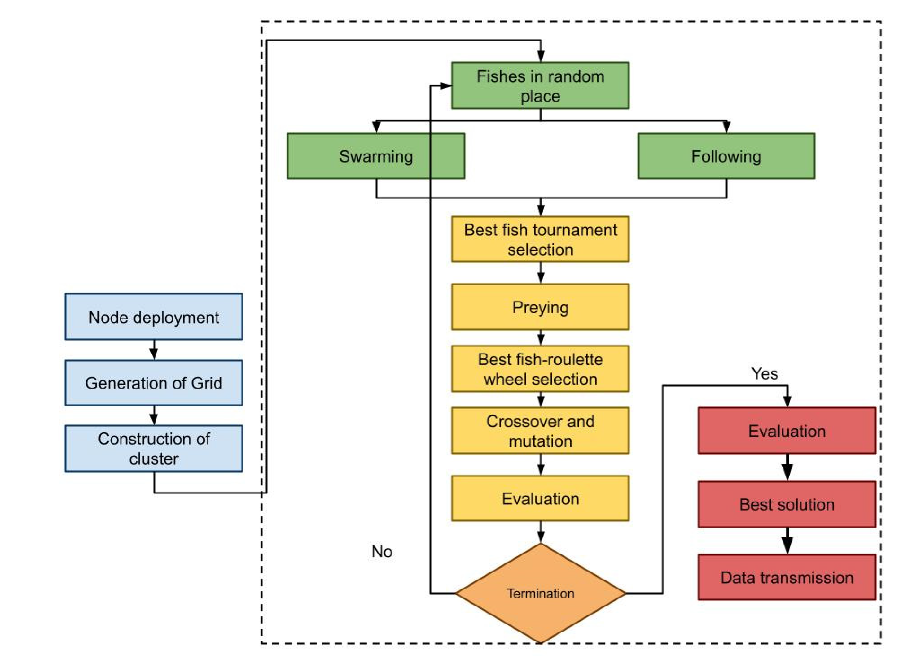
Grid cells of equal length are used to partition the whole network. Every grid cell represents the square territory. Every grid cell has only static nodes. The Sink can be either stationary or moveable for gathering data. The grid cell CH is the one that is closest to the mid-point of the grid cell. Every grid cell has a node ID as well as an associated grid ID that identifies nodes. The sink is responsible for the initial cluster setup, which includes calculating node IDs and grid IDs, establishing the CH for each grid cell and scheduling data transmission and reception for nodes in the grid cells. The GG-Conv_Clus-FSO protocol uses double disjoint anchor group nodes for packet forwarding, and node nomination is based on the clustering method. To locate holes quickly, a grid-based hole identification method is utilised. Data packets are accurately routed to the anchor and destination nodes while consuming the least amount of energy.

Grid Formation

The whole network is divided into equal-sized rectangle-shaped grid cells. Each grid keeps track of the exact location of each cell relative to its border, which is subsequently used to determine the size of the holes. In this, D_a × D_b denotes the grid cell dimension where the length is determined by D_a and width is determined by X_b. Equation (1) [31] indicates the grid cell generation process. The grid-building procedure is completed by

$$\mathrm{f}\left(\mathrm{g},\mathrm{r}\right)=\left(\left(g_0+\mathrm{g}\times D_a,r_0+\mathrm{r}\times D_b\right)\right)$$

(1)

where the count of a horizontal line is indicated by g, and the count of the vertical line is indicated by r. The process of grid construction is given in Algorithm 1.

Algorithm 1: Construction of Grid

for g = 0 to p = s

for r = 0 to r = t

$\mathrm{f}(\mathrm{g},\mathrm{r})=\left(\left(g_0+\mathrm{g}\times D_a,r_0+\mathrm{r}\times D_b\right)\right)$

end for

end for

Selection of Cluster Head (CH): In the actual world, fish can identify nutrient-rich places by searching on their own or by swimming near other fish; the region with the most fish often has the most nutrition. Artificial fish swarm optimization (AFSO) is based on mimicking fish behaviour, such as preying, swarming and tracking local fish hunts to attain global optima. The solution space and the states of other artificial fishes are generally the areas where an Artificial Fish (AF) dwells. The subsequent behaviour is determined by the current state as well as the immediate environment, such as the current quality of query responses and the status of nearby neighbours. The movements of an artificial fish, as well as the actions of its neighbours, have an impact on the ecosystem. If fish are discovered in a water area with more food, they will migrate quickly to that area. Equation (2) may be used to describe this behaviour.

$$F_v=F_i+Visual\times rand iϵ\left[0,n\right]$$

$$F_{next}=F+\frac{F_v-F}{||F_v-F||}\times step\times rand$$

(2)

During preying mode, fish behaviour is represented by Equation (3):

$$Prey\left(F_i\right)=\left\{\begin{array}{c}{f}_i+step\frac{f_j-f_i}{||f_j-f_i||} if y_j-y_i\\ f_i+\left(2rand-1\right).step else\end{array}\right.$$

(3)

where rand is the random function with range [0, 1].

The behaviour of the swarm is represented in Equation (4)

$$Swarm\left(F_i\right)=\left\{\begin{array}{c}{f}_i+step\frac{f_j-f_i}{||f_j-f_i||} if \frac{y_c}{nf}>\delta y_i\\ prey (f_i) else\end{array}\right.$$

(4)

In the follow stage, behaviour is given by equation

$$Follow\left(F_i\right)=\left\{\begin{array}{c}{f}_i+step\frac{f_{max}-f_i}{||f_{max}-f_i||} if \frac{y_{max}}{nf}>\delta y_i\\ prey (f_i) else\end{array}\right.$$

(5)

The three processes outlined above guarantee that both global and local searches are conducted, as well as a search direction that leads to the greatest food source. The suggested approach differs from the AFSA in two significant ways. The solutions are split at random and behave in one of two ways: swarming or following. The best fish are chosen via tournament selection, and preying processing begins. Fish who are very good at preying are chosen and allowed to breed amongst themselves. The best fish and the new solution are carried to the next iteration. The answers are represented as binary numbers in this study, and the distance between fish is calculated utilizing Hamming distance. The number of locations where two strings u and v differ is the hamming distance between them. The best fish are chosen by spinning the roulette wheel. The likelihood of a fish being picked on a roulette wheel is exactly proportional to its fitness. Equation (6) computes the probability of a fish,

$$p{b}_i=\frac{fi{t}_i}{{{\displaystyle \sum }}_{j=1}^{N}fi{t}_i}$$

(6)

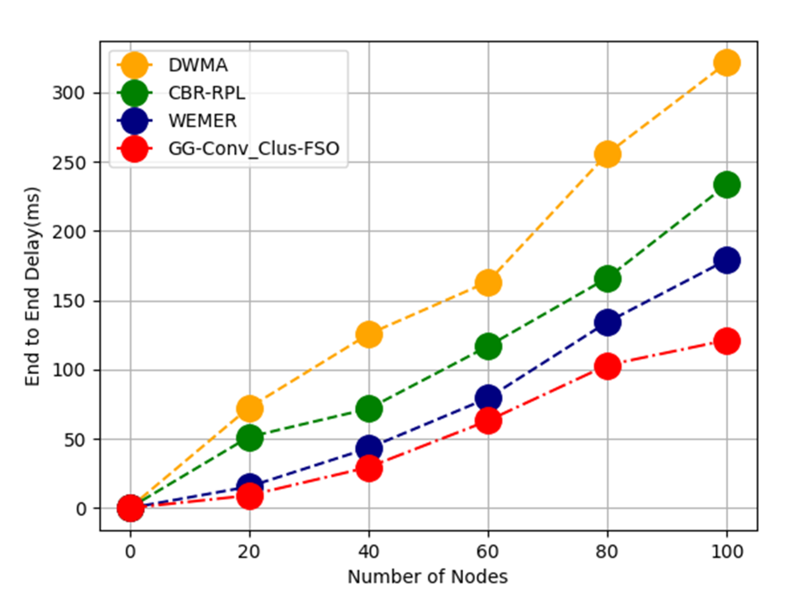
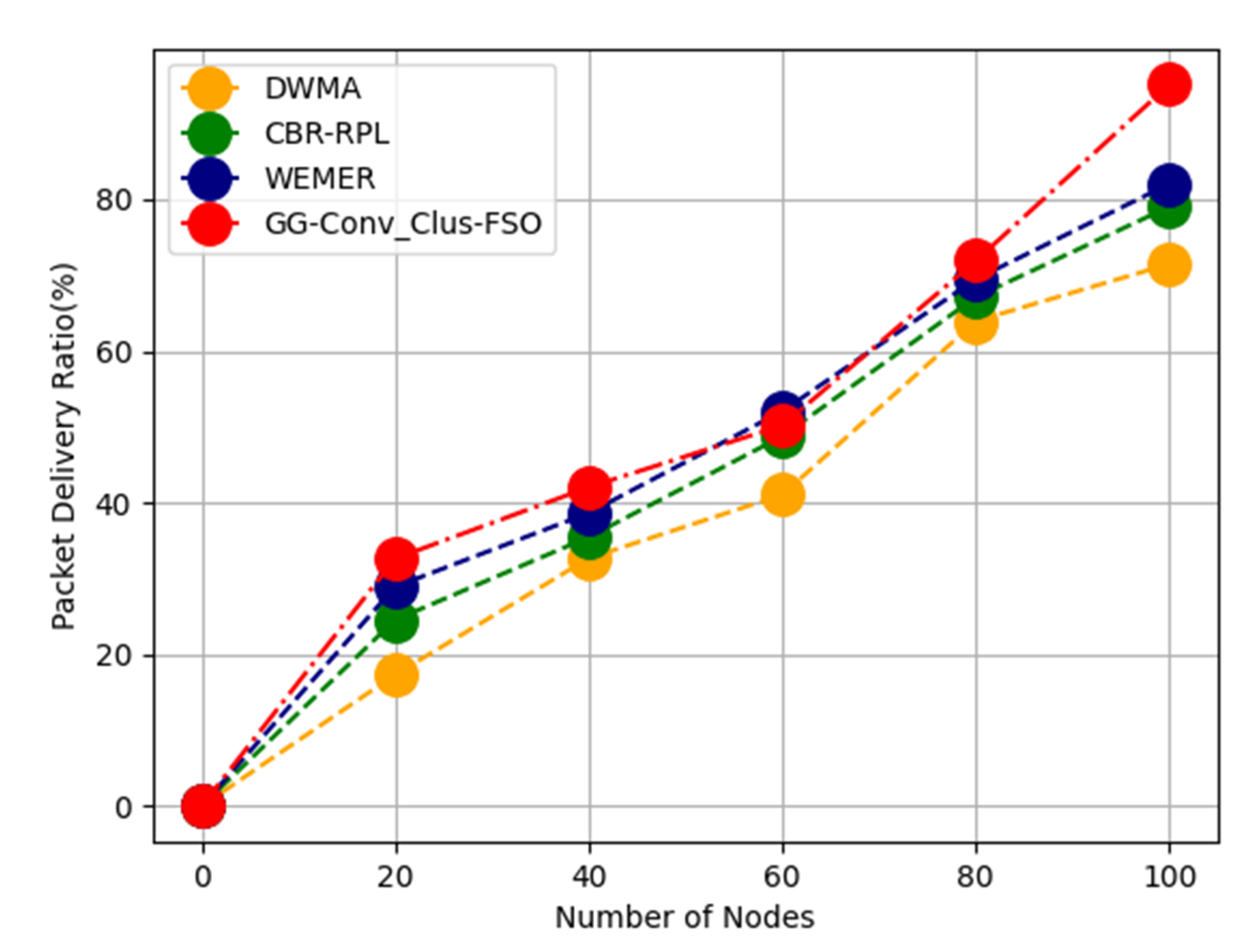
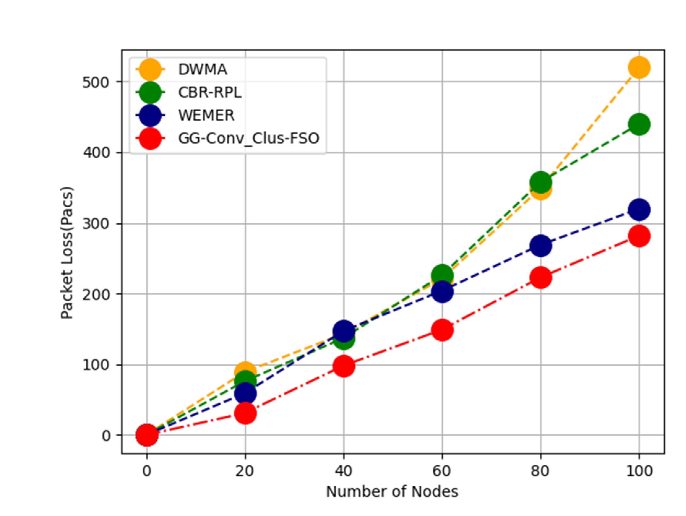
To enhance QOS, a multi-objective function based on E2E delay as well as energy is proposed and represented by Equation (7):

$$minfit\left(f_i\right)=\frac{e^{-\left(\frac{D_{td}}{D_m}\right)}}{\left(\frac{E_{ri}}{E_i}\right)}$$

(7)

where d_ri is the E2E delay, D_td is the total delay to reach BS, D_m is the maximum delay, E_ri is the remaining energy in CH and E_i is the initial energy.

Subsequent assumptions are made:

• The nodes in the network are distributed arbitrarily;
• Starting energy of every node is the similar;
• In ecology, all fishes are unisex;
• Because fish are unisexual, mating among any two fish is feasible;
• Because the free space radio method is utilised, the energy needed to transmit one bit of data grows as distance improves.

The flowchart for FSO-based CH selection is shown in Figure 1. Because solution space is binary, a transfer function is required to fill the bit as the fish swims. In this paper, a novel transfer function for flipping the bits described by Equation (8) is,

$$transfer\left(F_i\right)=\frac{1}{\left(1+e^{-\tan \mathrm{h}\left(f_i\right)}\right)}$$

(8)

To attain flipping, a random number between 0 and 1 is generated, and if the random number is less than the transfer function provided by Equation (8), the bit is flipped.

$$\left\{\begin{array}{c}1, if p\left(0,1\right)<transfer\left(F_i\right)\\ 0, otherwise\end{array}\right.$$

(9)

Hole Detection: The grid hole is found by comparing the cell coordinates to SNs radius as well as closest count (SN). SN count is closer to the sensor’s radius, which is used to determine the hole’s coverage area. The region in which a hole has developed is said to be B_i. Equations (10) and (11) show the position of the hole in the cell and the grid.

$$B_{cell }={\displaystyle \sum }_1^{i}Bi$$

(10)

$$B_{\mathrm{total}}={\displaystyle \sum }_1^{j}Bcell$$

(11)

Data propagation across selected CH: Send data around the borders of the hole and transfer it to the correct location. The sensor nodes in the region are clustered, and the CH is selected as the node closest to the grid’s centre. In the GBC-SS, the Static Sink is in charge of coordination, whereas in the GBC-MS, Mobile Sink is in charge of data gathering. The information is transmitted to nearby sensor nodes, and the position is recorded for future data transfer.

$$\mathrm{Load}\mathrm{in}\mathrm{the}\mathrm{CH}\mathrm{node}=\left(\frac{Whole CH communication cost}{ total cost of CH}\right)$$

(12)

$$\mathrm{Load}\mathrm{per}\mathrm{grid}\mathrm{cell}=\left(r^2\rho dt\right)$$

(13)

$$\mathrm{Intra}-\mathrm{and}\mathrm{inter}-\mathrm{cluster}\mathrm{communication}\cos \mathrm{t}=\left(r^2\rho dt\right)\times {{\displaystyle \sum }}_{i=1}^n\left(2i-1\right)gl1+{{\displaystyle \sum }}_{i=1}^n\left(2i-1\right)i$$

(14)

where the density is indicated by $\rho$, the transmission rate of data is characterized by a dot and the determined location is shown as gl.

$\mathcal{G}=\left(\mathcal{F},\mathcal{E},\mathcal{H}\right)$ is the definition of an undirected and connected graph, where V and E are finite sets of V = N vertices and edges, and $W\in {ℝ}^{\mathcal{N}\times \mathcal{N}}$ is an adjacency matrix. The graph signals are represented by numerous variables in each vertex. The description indices are represented by the vertex variables in this study. The graph is given by its Laplacian matrix L, which is defined as $\ell =D-W$, where $D=\mathrm{diag}\left({\dot{d}}_0,\dots ,d_{N-1}\right)$ is the degree matrix created by degrees $d_i={\sum }_j{W}_{i,j}$ of vertex i. represented as ${\left\{{\chi }_{\ell }\right\}}_{/=0}^{N-1}$ with corresponding nonnegative eigenvalues $0\le {\lambda }_0\le \dots \le {\lambda }_{N-1}$. Laplacian matrix L, is diagonalized by the eigenvector matrix $\mathcal{X}=\left[{\chi }_0,\dots ,{\chi }_{N-1}\right]$ so that $\ell =\mathcal{X}\Lambda {\mathcal{X}}^T$, where is the diagonal eigenvalue matrix. $\ell =I_N-D^{-1/2}\mathcal{𝒻}{D}^{-1/2}$ is a normalised version [1, 1].

Instead of complex exponentials, the eigenvectors ${\left\{{\chi }_{\ell }\right\}}_{/=0}^{N-1}$ of the Laplacian matrix L that meet the orthogonality criterion are employed as decomposition bases for graph-structured data. On a graph, the Fourier transform of a given signal f(n) is defined as Equation (15):

$$\hat{f}\left({\lambda }_l\right)={\sum }_{n=0}^{N-1}{\chi }_l^T\left(n\right)f\left(n\right)=X^{T}f$$

(15)

Inverse Fourier transformation is represented by Equation (16):

$$f\left(n\right)g\left(n\right);g\left(n\right){\left\{{\theta }_{,},\right\}}_{=0}^{N-1}\mathcal{G}\left(\Lambda \right).f$$

(16)

Convolution is turned into a point-wise product in the Fourier domain as well as reconverted into the vertex domain utilizing the graph Fourier transform as well as the convolution theorem, as in Equation (17):

$$f\times g=X({\sum }_{k=0}^K {\theta }_k{\Lambda }^k){\mathcal{T}}^{T}f=({\sum }_{k=0}^K {\theta }_k\left(X^{\top }{\Lambda }^k{X}^T\right))f={\sum }_{k=0}^K {\theta }_k{\ell }^{k}f$$

(17)

A convolution kernel is the graph convolution operation of two graph signals, f(n) and g(n), and its transform, $\mathcal{G}\left(\Lambda \right)$. A set of free parameters in the Fourier domain, i.e., Laplacian eigenspace, is used to construct this kernel. Convolution is then written as Equation (18):

$$\mathrm{f}*g=\mathcal{X}\mathrm{diag}\left({\theta }_0,\dots ,{\theta }_{N-1}\right){\mathcal{X}}^{T}f=\mathcal{X}\mathcal{G}\left(\Lambda \right){\mathcal{X}}^{T}f\mathcal{G}\left(\Lambda \right)$$

(18)

$\mathcal{G}\left(\Lambda \right)$ as an eigenvalue polynomial function: As illustrated in Equation (19), a rapid localised convolution based on low-order polynomial approximation was proposed:

$$G\left(\Lambda \right)={\sum }_{(k=0)}^K{\theta }_k{\Lambda }^k$$

(19)

which ${\left\{{\theta }_k\right\}}_{k=0}^K$ is the polynomial order, and Ki is a vector of polynomial coefficients. K is a tiny positive integer, such as 3, for example. Convolution is then rewritten as Equation (20):

$$f\times g=X({\sum }_{k=0}^K{\theta }_k{\Lambda }^k){\mathcal{T}}^{T}f={({\sum }_{k=0}^K}^K{\theta }_k\left(X^{\top }{\Lambda }^k{X}^T\right))f={\sum }_{k=0}^K{\theta }_k{\ell }^k$$

(20)

The convolution is performed by K multiplications of the sparse matrix L, which speeds up computation by avoiding the composition procedure.

The following is the updated version of Equation (21) for layer l:

$$\begin{gathered} {\hat{h}}_i^{l+1}=O_h^l{H}_{k=1}\left({\sum }_{j\in N_i}{w}_{i,j}^{k,l}{V}^{k,l}{h}_j^l\right) \\ {\hat{e}}_i^{l+1}=O_e^l{H}_{k=1}\left({\hat{w}}_{i,j}^{k,l}\right) \end{gathered}$$

where

$$w_{ij}^{k,l}=\mathrm{softmax}{x}_j\left({\hat{w}}_{i,j}^{k,l}\right)$$

(21)

$${\hat{w}}_{i,j}^{k,l}=\left(\frac{Q^{k,l}{h}_i^l\cdot K^{k,l}{h}_j^l}{\sqrt{d_k}}\right)\cdot E^{k,l}{e}_{i,j}^l$$

with $Q^{k,l},K^{k,l},V^{k,l},E^{k,l}\in R{d}_k,O_{h,}^l,O_e^l\in R^{d\times d},k\in \left\{1,2,\dots ,H\right\}$ relates the number of attention heads, and where $O_h^l\in R^{d\times d},V^{k,l}\in R^{d_k\times d},d_k$H denotes the number of heads. Note that h l i is i-th node’s feature at l-th layer in Equation (22).

$$\mathrm{cut}(S_k,S_k)=\sum _{v_i\in S_k,v_j\in S_j}e(v_i,v_j),$$

(22)

where $S_k$ is k-th set of a given graph, ${\hat{S}}_k$ indicates the remaining sets, except $S_k$, and $e\left(v_i,v_j\right)$ is the edge between vertices $v_i$ and $v_j$. When referring to multiple sets, the cut issue is represented as Equation (23):

$$\mathrm{cut}(S_1,S_2,S_3\dots S_8)=\frac{1}{2}\sum _{i=k}^8\mathrm{cut}(S_k,S_k)$$

(23)

The issue of less cuts is extensively studied in the literature in Equation (24):

$$\mathrm{Ncut}(S_1,S_2\dots S_g)=\sum _{k=1}^g\frac{\mathrm{cut}(S_k,{\hat{S}}_k)}{\mathrm{vol}(S_k,V)},$$

(24)

where $\mathrm{vol}(S_k,V)\sum =v_i\in S_k,v_i\in v^e(v_i,v_j)$ is the total degree of nodes from $S_k$ in graph $g$. The normalised cut problem utilizing DL optimisation, transforming the minimum cut issue into a DL format, as in Equation (25):

$$L_{\mathrm{cut}}={\sum }_{\mathrm{reduce}\_\mathrm{sum}}(Y\oslash \Gamma ){(1-Y)}^T\odot A+{\sum }_{\mathrm{reduce}\_\mathrm{sum}}{(1^{T}Y-\frac{n}{g})}^2$$

(25)

A is the adjacency matrix, and, finally, Γ is evaluated by Equation (26):

$$H_j^{[l+1]}=\sigma (\sum _{i=1}^{F_{in}}(\sum _{k=0}^K{\theta }_{i,j_k}{\ell }^k{H}_i^{\left[l\right]})+b_j^{\left[l\right]})$$

(26)

where (·) relates a non-linear activation function, e.g., ReLU (·) max(0, ·) = ; Hi [ ]l indicates ith input graph; ijk, and bj [ ] l are trainable F F in out × vector of K-order polynomial coefficients and 1 × Fout vector of bias in l th layer.

4. Result and Discussion

In this section, the simulation outcome of the proposed Graph-Grid-based Convolution clustered neural network with fish swarm optimization (GG-Conv_Clus-FSO) is compared with the existing techniques such as DWMA for 6LowPAN RPL, CBR-RPL, CCS and WEMER and PEGASIS. The simulation of the above-mentioned approaches is investigated with the assistance of the number of rounds vs. alive nodes, the number of rounds vs. dead nodes, PDR, energy consumption and delivery delay. The simulation setup is given in

Table 1. Simulation Setup.

Parameters	Values
No. of nodes	200
Simulation area	1000 × 1000 m2
Routing protocol	RPL
Initial energy	100 Joule
Packet size	300 bits
Simulation time	65 ms

.

4.1. Energy Consumption

Every sensor node in the data transmission environment in the WSN is equipped with rechargeable batteries that consume the least amount of energy, making battery recharging difficult. The cluster and duty cycle scheduling mechanisms start the data transfer. The data transmission process is completed without interruption, and data are transmitted in the quickest way possible while consuming the least amount of energy. The transmission nodes’ energy consumption is minimized as a result of this condition is given in

Table 2. Comparison of energy consumption.

No of Nodes	DWMA	CBR-RPL	WEMER	GG-Conv_Clus-FSO
0	0	0	0	0
20	5.12	3.47	2.49	1.08
40	12.17	9.22	4.13	3.42
60	25.46	13.79	5.43	4.79
80	31.45	19.47	8.24	6.33
100	43.78	29.55	11.85	7.04

.

In Figure 2, energy consumption during data transmission for a different number of nodes is illustrated. The energy consumption of the proposed approach is minimal than existing approaches, namely DWMA, CBR-RPL, WEMER and PEGASIS.

4.2. End to End Delay

It is time takes to transport data from source to destination node. A protocol that has the shortest transmission delay is considered to be effective, the comparisons are given in

Table 3. Comparison of end-to-end delay.

No of Nodes	DWMA	CBR-RPL	WEMER	GG-Conv_Clus-FSO
0	0	0	0	0
20	72.49	51.34	15.46	9.13
40	125.44	71.66	43.21	29.47
60	163.27	116.77	79.34	63.06
80	255.79	166.06	134.29	103.22
100	321.44	233.45	179.11	121.19

.

In Figure 3, end-to-end delay during data transmission for various numbers of nodes is illustrated. E2E delay of the proposed technique is minimal than existing approaches, namely DWMA, CBR-RPL, WEMER and PEGASIS.

4.3. Packet Delivery Ratio

PDR is determined by dividing the total number of data packets sent from source to destination node by the number of data packets delivered. Data communication technology that delivers most packets is deemed the best. The packet delivery ratio of the different method is mentioned in

Table 4. Comparison of the packet delivery ratio.

No of Nodes	DWMA	CBR-RPL	WEMER	GG-Conv_Clus-FSO
0	0	0	0	0
20	17.32	24.55	28.91	32.63
40	32.67	35.46	38.64	42.03
60	41.04	48.75	52.06	50.17
80	63.93	67.11	69.47	71.90
100	71.46	79.02	82.03	95.14

.

In Figure 4, PDR during data transmission for different numbers of nodes is illustrated. PDR of the proposed approach is higher than existing approaches, namely DWMA, CBR-RPL, WEMER and PEGASIS.

4.4. Packet Loss

Packet loss can be triggered by a mixture of circumstances, including signal deterioration owing to multi-path fading on the network media. In WSNs, packet loss is conceivable. In order for attackers to simply acquire the data. Packet loss occurs when one or more sent packets fail to reach their intended destination. The Packet Delivery Ratio is reduced when packets are lost. The packet loss of the different method is compared and its mentioned in

Table 5. Comparison of packet loss.

No of Nodes	DWMA	CBR-RPL	WEMER	GG-Conv_Clus-FSO
0	0	0	0	0
20	89	76	59	31
40	143	137	147	98
60	221	226	204	149
80	349	358	269	223
100	520	440	320	282

In Figure 5, packet loss during data transmission for different number of node is illustrated. The packet loss of proposed approach is minimal than existing approaches, namely DWMA, CBR-RPL, WEMER and PEGASIS.

4.5. Throughput

The amount of data that is efficiently sent/received through a communication channel is referred to as throughput. Throughput is calculated in kilobits per second, megabits per second or gigabits per second and might differ from bandwidth owing to a variety of technical issues such as packet loss, latency, jitter, and more. The quantity of data that is moved from one location to another in a given length of time is referred to as throughput. The comparisons of previous methods and proposed method is mentioned in the below

Table 6. Comparison of throughput.

No of Nodes	DWMA	CBR-RPL	WEMER	GG-Conv_Clus-FSO
0	0	0	0	0
20	65.22	87.24	98.53	127.43
40	127.42	154.36	187.25	206.33
60	178.11	221.42	267.22	281.16
80	229.55	265.86	298.45	379.55
100	276.34	321.46	357.11	465.51

.

In Figure 6, the throughput during data transmission for different numbers of nodes is illustrated. The throughput of the proposed approach is minimal compared to the existing approaches, namely DWMA, CBR-RPL, WEMER and PEGASIS.

5. Conclusions

The Internet of Things has a significant influence on daily living. For IoT and LLNs, the RPL has become the standard protocol. It is not only extensively utilised, but it has also been studied by diverse groups of individuals. The widespread usage of RPL and its customisation has necessitated substantial study and development. There are certain flaws with the existing RPL mechanism, one of which is an energy hole, which is a major problem in the context of IoT. Fish swarm optimization is used to initiate Grid creation among sensor nodes, which can help in cluster formation and Cluster Head (CH) selection with energy optimization by calculating the energy consumption of the network. The performance of a Graph-Grid-based Convolution clustered neural network with fish swarm optimization (GG-Conv_Clus-FSO) is compared to existing state-of-the-art protocols, and the GG-Conv_Clus-FSObeats the existing techniques, with a 95.14 percent increase in the packet delivery ratio (PDR).