Article

Intelligent Modeling of the Incineration Process in Waste Incineration Power Plant Based on Deep Learning

1
Shenzhen Energy Environment Engineering Co., Ltd., Shenzhen 518048, China
2
School of Control and Computer Engineering, North China Electric Power University, Baoding 071003, China
*
Author to whom correspondence should be addressed.
Energies 2022, 15(12), 4285; https://doi.org/10.3390/en15124285
Submission received: 1 May 2022 / Revised: 6 June 2022 / Accepted: 10 June 2022 / Published: 10 June 2022

Abstract

:
The incineration process in waste-to-energy plants is characterized by high levels of inertia, large delays, strong coupling, and nonlinearity, which makes accurate modeling difficult. Therefore, an intelligent modeling method for the incineration process in waste-to-energy plants based on deep learning is proposed. First, the output variables were selected from the three aspects of safety, stability and economy. The initial variables related to the output variables were determined by mechanism analysis and the input variables were finally determined by removing invalid and redundant variables through the Lasso algorithm. Secondly, each delay time was calculated, and a multi-input and multi-output model was established on the basis of deep learning. Finally, the deep learning model was compared and verified with traditional models, including LSSVM, CNN, and LSTM. The simulation results show that the intelligent model of the incineration process in the waste-to-energy plant based on deep learning is more accurate and effective than the traditional LSSVM, CNN and LSTM models.

1. Introduction

At present, the treatment methods for domestic waste usually include landfill, compost and incineration [1,2]. According to the statistics and the volume of domestic waste removal and transportation, the proportion of landfill treatment, compost treatment and incineration treatment is 58.30%, 2.10% and 36.20% respectively, and the remaining 3.40% are treated by simple landfill and stacking [3]. However, due to problems such as the large amount of land required and environmental pollution, the proportion of landfill treatment and compost treatment is decreasing year by year. The waste incineration process reduces the content of harmful substances in the waste by pyrolysis and oxidation under high temperature and high pressure. The volume of waste after incineration is reduced by more than 85% and the weight is reduced by more than 75%. The waste incineration process greatly eliminates the germs and harmful components in the waste, thus achieving the efficient treatment of the waste. Additionally, the energy generated by incineration can be used to generate electricity to realize a major goal of waste recycling [4]. It has been suggested that waste incineration power generation technology has the advantages of “reduction, recycling, and harmlessness”, and that it is currently the best way to deal with domestic waste [5]. However, due to the complex composition of waste, the large fluctuations in waste calorific value, and the fact that the incinerator is a multi-input and multi-output (MIMO) object distinguished by high levels of inertia, large delays, strong coupling, and nonlinearity, it is difficult to meet the needs of the subsequent combustion optimization. Therefore, establishing an accurate and reliable intelligent model of the incineration process of waste-to-energy plants is the key to subsequent incineration optimization [6,7].
Elisa [8] et al. used the mechanism modeling method to model the incineration process of waste-to-energy power plants, but there were problems related to the complicated derivation process and low precision. Therefore, data-driven modeling has been widely used in combustion process modeling [9,10]. Peng et al. [11] established a multi-input and single-output model for boiler combustion oxygen content based on big data and a neural network, and enhanced the neural network through Bayesian arithmetic, which solved the problem of slow learning speed and the problem of obtaining the optimal value in a small range of the classical neural network. Based on the operating data for a boiler in a thermal power plant, Song et al. [12] used a radial basis neural network to establish a model with the flue gas oxygen content, furnace negative pressure and steam pressure as outputs. Compared with a back propagation (BP) neural network, a radial basis function (RBF) neural network has better categorization capability, approximation ability and learning speed, but it has poor resistance to noise in the sample data. Zhong et al. [13] used the particle swarm algorithm and support vector machine to establish a boiler exhaust gas temperature model of a 660 MW unit, which provided guidance for the operation of the boiler. However, for large amounts of sample data, support vector machines are prone to overfitting and lack modeling accuracy. Due to the structural limitations of the algorithms themselves, these algorithms cannot mine the deep information in the sample data [14].
With the rapid development of artificial intelligence, modeling methods based on deep learning have attracted more and more scholars’ attention. Hu et al. [15] established a boiler combustion efficiency model using a convolutional neural network for a 600 MW supercritical unit boiler in Henan. Yu et al. [16] used deep CNN and support vector machine to extract and analyze the deep features of flame images, and realized the modeling of the NOx concentration of a 4.2 MW heavy oil combustion boiler. Zhang [17] established a deep neural network model of a stacking noise reduction autoencoder and LSTM network considering the characteristics of ultra-supercritical units such as high inertia, large delays and noise in the actual data. However, the existing modeling methods generally have defects such as too few input and output variables, which are far from the actual operation of the actual unit, and the inability to express the dynamic characteristics of the model. Therefore, in the process of model establishment, in addition to selecting the modeling method, the selection of input variables will also affect the modeling accuracy. Wang et al. [18] utilized principal component analysis means to lower the dimension of the multi-dimensional input variables of wind turbines. Although the feature dimension was reduced, the original data was changed and the interpretability of the model was reduced.
Incinerator incineration process modeling data are characterized as complex large sample data, nonlinear time series, etc. Compared with the methods described above, the deep learning network method can use the complexity relationship between data to automatically model and adjust the model parameters so as to establish the optimal nonlinear model between input and output. That is, this method is able to use the time series’ characteristics or other complex relationships between historical data to model through deep learning networks. In summary, an intelligent model of the incineration process of waste-to-energy plants based on deep learning is elicited. First, the output variables are selected from the three aspects of safety, stability and economy. The initial variables related to the output variables are determined. The input variables were finally determined by removing the invalid variables and redundant variables through the Lasso algorithm. Secondly, each delay time is calculated, and a multi-input and multi-output model based on deep learning is established. Finally, the model proposed in this paper is compared with the traditional model to verify the improvement in its accuracy.

2. Basic Method Principle

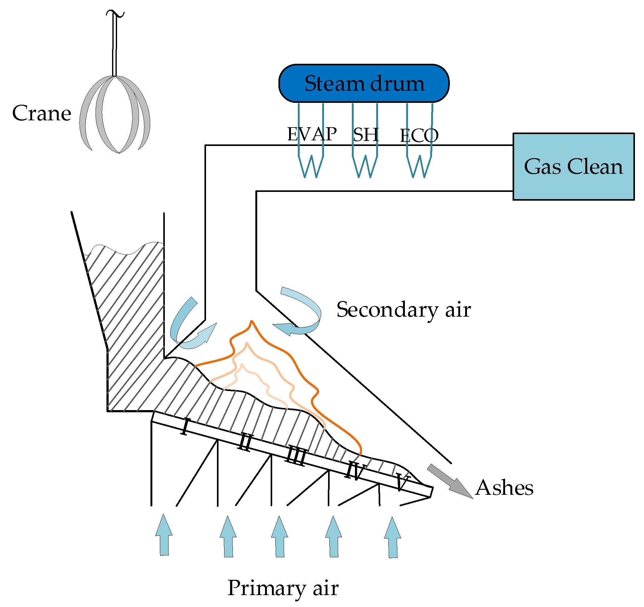
2.1. Waste-to-Energy Treatment Technology

After the garbage is transported to the incineration plant, it is fermented in a garbage storage tank for 3–5 days to increase the calorific value. The calorific value of the waste after fermentation is about 1800–2100 kcal/kg. Garbage fermentation mainly relies on the role of microorganisms in the garbage. At the same time, during the storage of the garbage, the water in the garbage is continuously leached out. After storage and fermentation, the garbage is moved to the feeding hopper by a hanging garbage grab, and is transported to the incinerator through the feeding grate. The incinerator is composed of a multi-stage mechanical grate, of which the first and second stages of the incineration grate are the waste drying area, the third and fourth stages of the incineration grate are the waste gasification area (main combustion area), and the fifth stage is the burning ember area. At the same time, each section of the combustion grate includes a fixed grate, sliding grate and turning grate. The sliding grates slowly push the garbage layer forward on the grate, and the function of the turning grate is to drive the overturning grate pieces to turn up and down through the reciprocating rotation of the overturning shaft, so as to support the garbage bed in a local position, destroy the original garbage bed, cause the previously formed bed to dislocate, and break the hard-shell surface and molten layer caused by burning. The primary combustion air is blown into the interior of the garbage bed (like throwing a fire) so that the garbage can be completely burned. The fan system consists of a primary air system, secondary air system and furnace-wall-cooling air system, among the first two wind systems that affect the combustion process. The primary air is extracted from the garbage storage tank, heated to about 180 °C by the air preheater, and sent to the bottom of the incinerator through the gap between the grate pieces of the incinerator. Then it penetrates the garbage bed and enters the incinerator chamber, where it is mixed with the garbage and burns. At the same time, a negative pressure in the garbage pond is established to prevent the overflow of garbage odor, so as to achieve effective management of odor. The secondary air mainly adjusts the amount of oxygen to ensure better combustion conditions. In view of the characteristics of China’s garbage, which has high moisture content, high non-combustible content and low calorific value, the design of the rear arch of the furnace is adapted, as shown in Figure 1, to form a good aerodynamic field and help combustion [19].

2.2. Lasso Algorithm

Least absolute shrinkage and selection operator (Lasso) is a penalty-based variable selection method first proposed by the famous statistician Robert Tibshirani in 1996 [20,21]. The specific principle is as follows.
The following is an example of a typical linear regression model:
y i = β 0 + j = 1 p x i j β j + e i i = 1 , 2 , , n
There are n sets of observations, and each group of observations consists of an input variable y i and p-correlated predictor variables x i = ( x i 1 , x i 2 , , x i p ) T .
The traditional method is to minimize the least squares objective function:
min m i z e β 0 , β i = 1 n ( y i β 0 j = 1 p x i j β j ) 2
In the general formula, the least squares estimation of β is not 0, and if n < p, there are countless solutions that make the objective function 0, hence the result of the least squares estimation is not unique. Therefore, this process needs to introduce a penalty function, that is, regularization. The Lasso algorithm is based on the least squares estimation to introduce a penalty factor to constrain the norm of β, as shown in the formula.
R S S ( β ^ ) = arg min β ^ i = 1 n ( y i β 0 j = 1 p β j x i j ) 2 + λ j = 1 p | β j | β ^ = arg min { y β 0 x β 2 2 } s . t β t
In the formula, λ 0 is the hyperparameter, λ j = 1 p | β j | is the compression penalty, t is the adjustment parameter, and the inequality β t effectively restricts the parameter space and realizes feature selection.

2.3. Model Building Based on Deep Learning

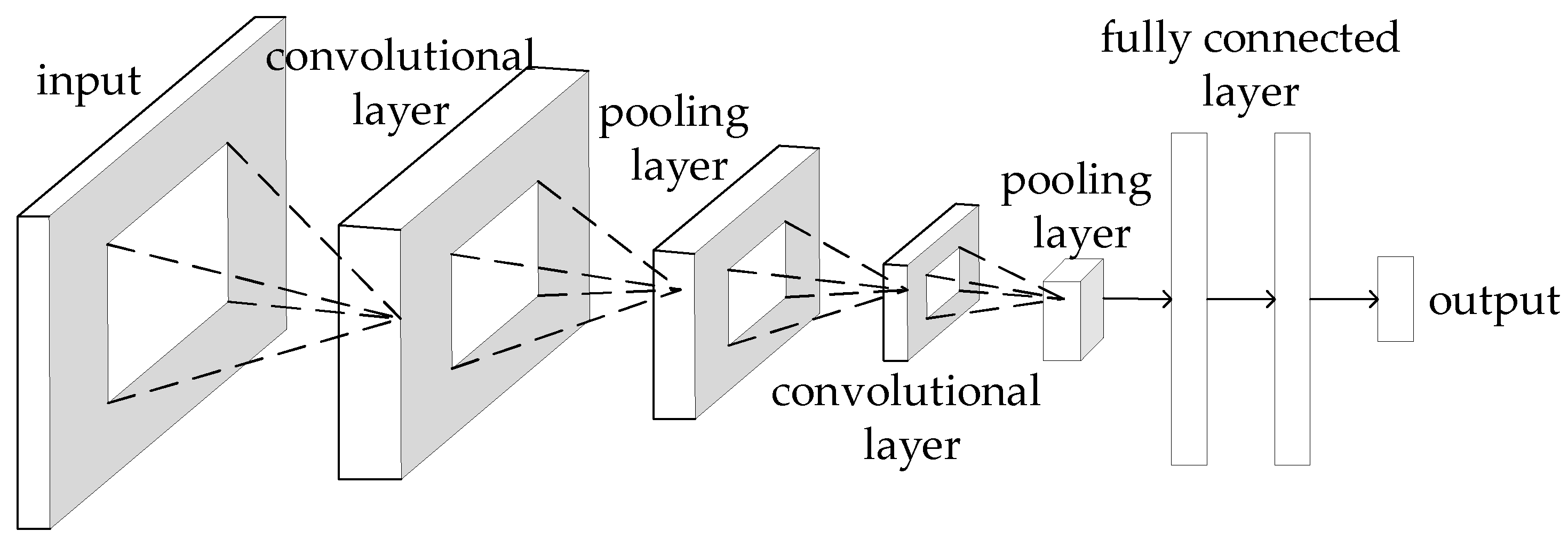
2.3.1. Convolutional Neural Network

CNN is a feedforward network that was first used in image processing and has excellent performance [22]. CNN has the characteristics of weight sharing, local connection, and dimensionality reduction sampling, and can fully mine the local characteristics of the data itself.
CNN generally contains three basic layers: a convolutional layer, pooling layer and fully connected layer. The pixels in the local area of the input image are weighted by the weight coefficient of the convolution kernel, the operation of feature extraction is completed by the convolution layer, and the activation function introduces nonlinear changes to the network model. The pooling layer performs dimension reduction sampling on the output of the convolutional layer, and at the same time, the pooling operation results in translation invariance in the CNN. The fully connected layer is where each node is linked to all the nodes in the previous layer, which is used to synthesize the features extracted in the front, as depicted in Figure 2.
This paper uses CNN to fully mine the features of the data, and the feature data processed by the convolution operation is sent to the Bi-LSTM network for further operations.

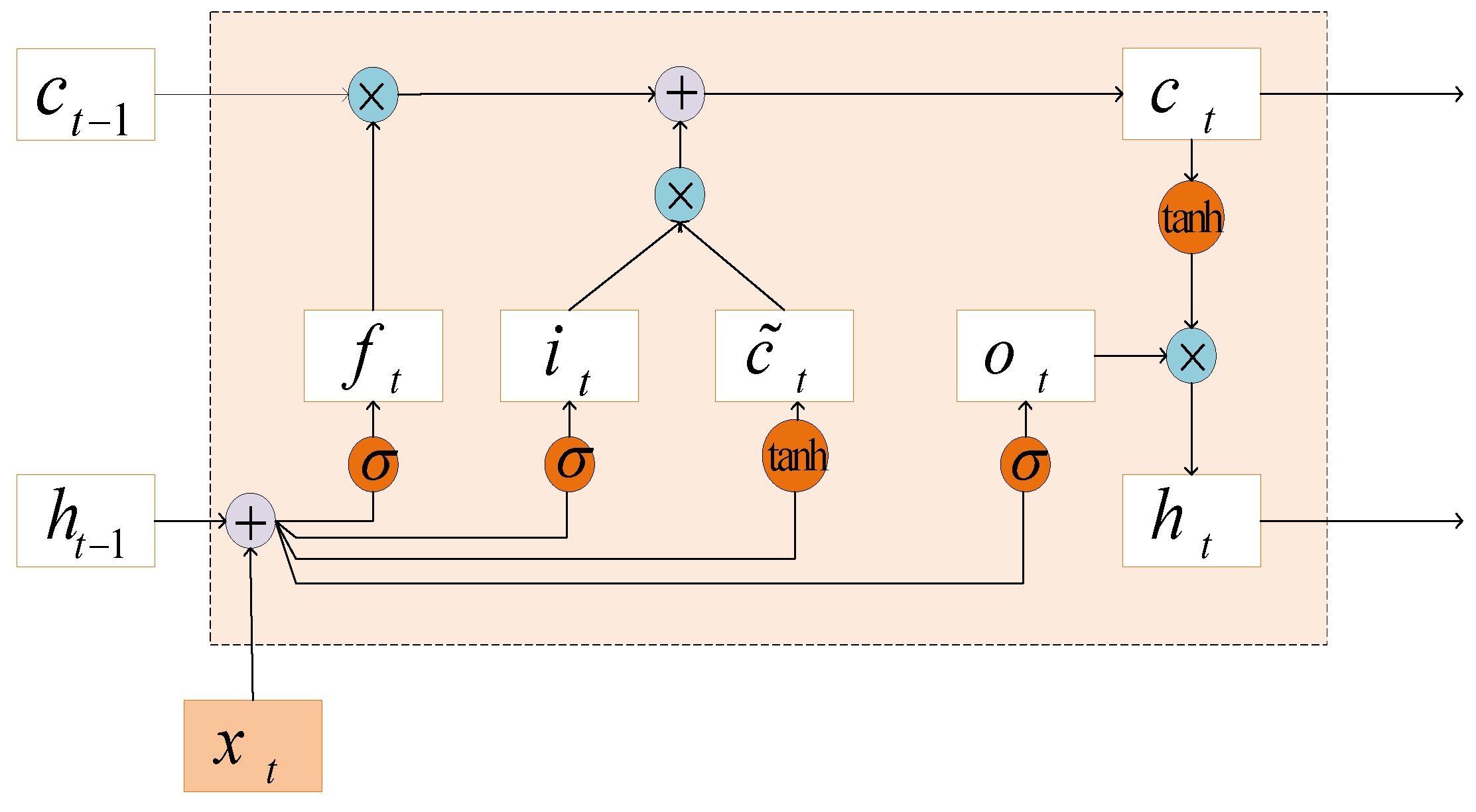
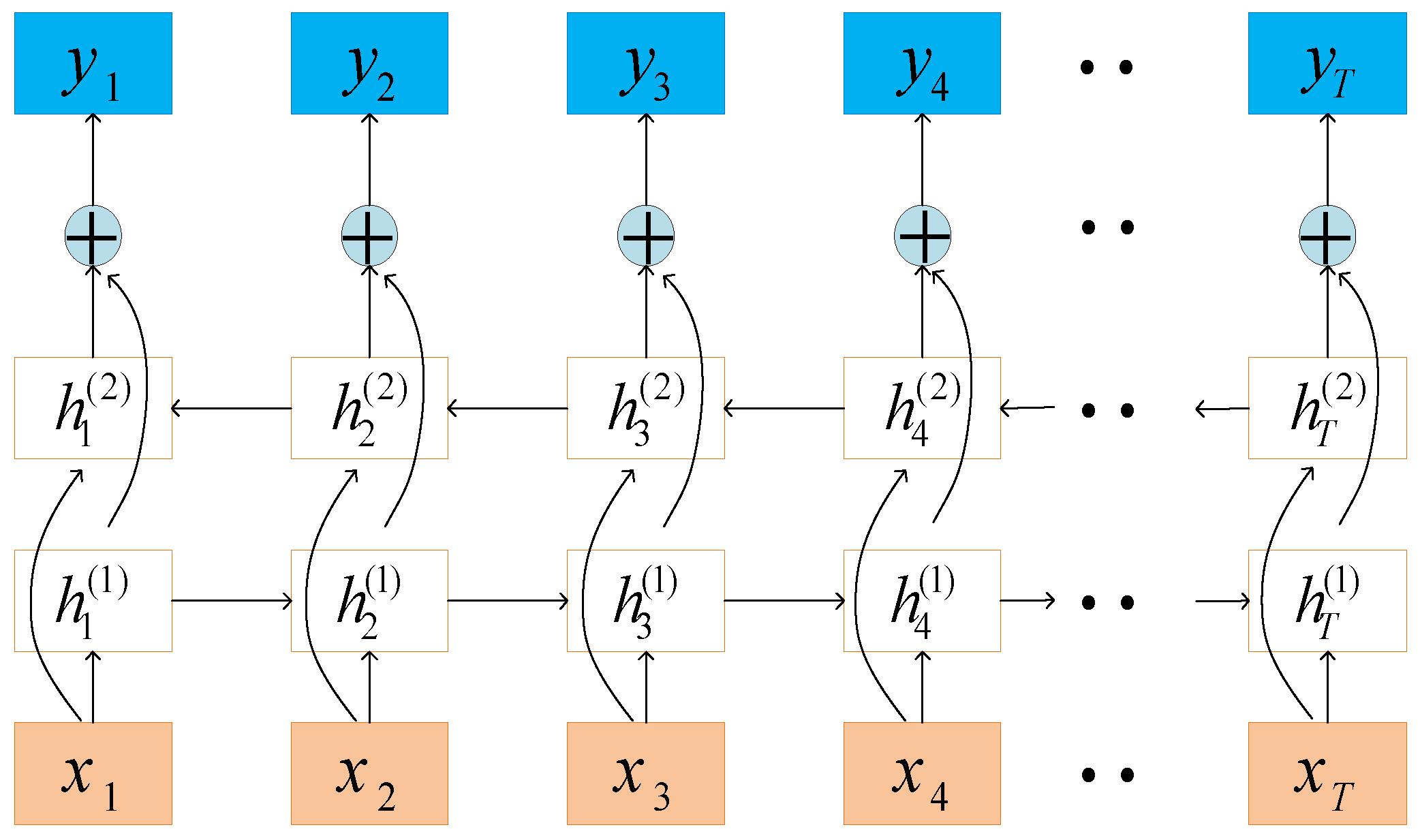
2.3.2. Bi-LSTM Model

The cyclic unit construction of LSTM is exhibited in Figure 3.
[ c ˜ t o t i t f t ] = [ tanh σ σ σ ] ( P [ x t h t 1 ] + b )
i t = σ ( P i x t + Q i h t 1 + b i )
f t = σ ( P f x t + Q f h t 1 + b f )
o t = σ ( P O x t + Q o h t 1 + b 0 )
c t = f t c t 1 + i t c ˜ t
c ˜ t = tanh ( P c x t + Q c h t 1 + b c )
h t = o t tanh ( c t )
First, use the input x t at the present moment and the external condition h t 1 at the previous moment to calculate f t , i t , o t and c ˜ t . Secondly, use f t and i t to update the memory unit c t , and finally, pass the internal state information to the external state h t in combination with o t [23].
LSTM can only extract forward sequence information, while Bi-LSTM (Bidirectional Long Short-Term Memory) extracts sequence information in both directions to obtain more data features [24]. Bi-LSTM consists of two layers of LSTM networks with the same input and different information transfer directions. The Bi-LSTM structure is shown in Figure 4.
h t ( 1 ) = f ( U ( 1 ) h t 1 ( 1 ) + W ( 1 ) x t + b ( 1 ) )
h t ( 2 ) = f ( U ( 2 ) h t + 1 ( 2 ) + W ( 2 ) x t + b ( 2 ) )
h t = h t ( 1 ) h t ( 2 )
is the vector concatenation.

2.3.3. Intelligent Model of Incineration Process Based on Deep Learning

The CNN-BiLSTM combined model not only combines the feedforward mechanism of the CNN with the feedback mechanism of the RNN, but also greatly reduces the computational cost through feature extraction of the CNN. Furthermore, by combining the models with BiLSTM, the model accuracy is improved.
Unlike steady-state modeling, dynamic models take into account the effects of time [25]. In the dynamic model of the CNN-BiLSTM incineration process, the output is not only related to the current data of each auxiliary variable, but also related to the delay time of the input and output variables [26].
In describing the dynamic characteristics of the waste incinerator combustion process, due to the existence of the delay time d, the sampling point at time t can be represented as { x ( t d ) , y ( t ) } . By discretizing the dynamic model of the incineration process, the difference equation form of the dynamic model is obtained as:
y ( t ) = f [ y ( t 1 ) , y ( t n ) , x ( t d ) ]
The above formula can be expressed as an intelligent model of the incineration process of waste-to-energy plants, which is a MIMO model. From the above equation, the output variable of the model can be obtained and is shown as the relationship of the output values of n past moments and the input values of d past moments.

3. Intelligent Model of Waste-to-Energy Plant Incineration Process Based on Deep Learning

3.1. Variable Selection Based on the Lasso Algorithm

Before building an incineration model, the input variables and output variables of the model should be determined. In this paper, the selection of the output variables of the intelligent model of waste-to-energy plant incineration process took the three aspects of safety, stability and economy into consideration. The output variables are the oxygen content of the boiler flue gas outlet ( C O 2 ), steam flow (Q), the furnace temperature of the incinerator (T1), and the temperature of the ember section (T2). The amount of oxygen is related to the load, and the amount of oxygen is used as a precursor to load changes. When the oxygen feedback value is higher than the set value, it means that the air volume is excessive or the garbage calorific value is insufficient. At this time, the boiler load decreases. When the oxygen feedback value is lower than the set value, the boiler load will increase. At this time, the boiler load should be reduced. If the oxygen content is lower than a certain level, it means that there is an abnormal situation such as an explosion in the furnace. At this time, the feeding should be stopped to prevent the garbage in the furnace from deflagrating and causing danger. When the steam flow is stable, this ensures that the steam turbine and generator work at the rated load and the equipment performance is good. Ensuring that the furnace flue gas stays above 850 °C for 2 s can prevent the generation of harmful flue gas dioxins. The temperature of the ember section is maintained within a certain range, which ensures that the garbage is fully burned and improves the combustion efficiency.
Mechanism analysis was used to select the input variables that have an impact on the output variables. A total of 19 variables related to the output variables were screened out from the variables collected by the power plant, namely, primary air flow, the temperature of primary air, unit 1–5 primary air flow, secondary air flow, the temperature of secondary air, unit 1–5 material layer thickness, the transmission speed of the sliding grate unit 1, the transmission speed of the sliding grate unit 2, the transmission speed of the sliding grate unit 3, the transmission speed of the sliding grate unit 4, and the transmission speed of the sliding grate unit 5. Since the secondary air temperature basically does not fluctuate, and there is a coefficient relationship between the transmission speeds of the five units of the sliding grate, 19 variables were screened and 14 initial variables were obtained.
The 14 initial variables were selected by the Lasso algorithm, and 8 input variables were finally obtained, namely, primary air flow, unit 1 primary air flow, unit 4 primary air flow, unit 5 primary air flow, secondary air flow, unit 1 material layer thickness, material layer thickness of unit 5, and conveying speed of sliding grate unit 1. Then, 25,200 sets of data were selected from a northern waste power plant from 16:00 on 6 August 2019 to 10:00 on 8 August 2019, and the sampling time was 6 s. The unit and variation range of each input variable are shown in Table 1. The local trend diagrams of the input variables are shown in Figure 5.

3.2. Calculation of Delay Time

Waste-to-energy generating units typically have large delays, and there is a time delay between the various data collected by the power plant. When an input variable changes, it takes a while for the output variable to react to the change. In order to ensure the consistency of each input variable and output variable in the time sequence, a time delay compensation algorithm based on mutual information is proposed. Mutual information can calculate the correlation between the two groups of samples. By determining the mutual information numerical value between the input variables and the output variables, the delay time between the input variables and the output variables can be obtained (the specific process can be found in [26]). Taking the steam flow as the output as an example, Table 2 shows the maximum mutual information of each input variable for the steam flow and the corresponding time delay at this time.

3.3. Model Establishment

The steps to build an intelligent model of the incineration process of a waste-to-energy plant are as follows:
(1)
The initial variables are screened by mechanism analysis and the Lasso algorithm, and invalid variables and redundant variables are removed.
(2)
Data preprocessing, including outlier removal, noise reduction, and normalization.
(3)
The mutual information method is used to determine each delay time.
(4)
The model is established: first, the input variables after feature selection are input into the CNN layer of the model, and the deep time series features are extracted through the convolution and pooling layers. Secondly, they are sent to the BiLSTM layer to further strengthen the connection between the temporal features. The last layer is the fully connected layer, and the model output is completed.
The CNN-BiLSTM model structure includes: 1 CNN, 1 max pooling layer, 1 dropout layer, 2 BiLSTM layers, and 1 fully connected layer. The parameters of the final training model are: the batch size is 128, epochs are 50, and the Adam optimization algorithm is selected.
In Figure 6, u is the initial variable, x is the input variable after variable selection, dij is the delay time between the input xi and the output yj, Y is the actual value, and Y ^ is the model output value.
The model building process is shown in Figure 6.

4. Model Establishment and Result Analysis

4.1. Model Evaluation Indicators

The model evaluation indicators used in this paper are MAE, MAPE, and RMSE. The closer the value is to 0, the more accurate the output of the model. The calculation formula is as follows:
M A E = 1 n i = 1 n | y i y ^ i |
M A P E = 1 n i = 1 n | y i y ^ i y i | × 100 %
R M S E = i = 1 n ( y i y ^ i ) 2 n
where y i is the actual sample value, y ^ i is the model output value, and n is the amount of data.
MAE reflects the magnitude of the deviation of the measured value from the true value; MAPE reflects the degree to which the sample output value deviates from the measured value; and RMSE reflects the sample standard deviation of the bias between the model output value and the measured value, reflecting the degree of dispersion of the sample. The combination of the three can better represent the precision of the model.

4.2. Model Establishment Result Analysis

.To test and verify that the output of the model is accurate, the first 90% of the 25,200 sets of data were used as the training set and the last 10% ere used as the test set in chronological order. Before the data is entered into the model, the data should be normalized to eliminate the influence of the input variables on the output of the modeling results due to different magnitudes and speeding up the running time of the model.

4.2.1. The Influence of Variable Selection on Modeling Results

There were still invalid variables and redundant variables in the variables obtained after the mechanism analysis. So as to solve the issue of model overfitting and further simplify the model, the Lasso algorithm was used for variable selection. Experiments were executed on the 14 initial variables obtained from the mechanism analysis and the 8 input variables selected by the Lasso algorithm to verify that the output of the model was accurate. The final evaluation indexes are revealed in Table 3.
It can be seen from Table 3 that after the selection of the initial variables, the test set error decreased. This phenomenon shows that since there are invalid variables and redundant variables in the initial variables, if these variables continue to be retained in the input variables, the generalization ability of the model will be reduced. Therefore, it is more efficient to select the variables before building a model as this not only simplifies the model and reduces the computing time during modeling, but also prevents the model from overfitting and improves the model accuracy.

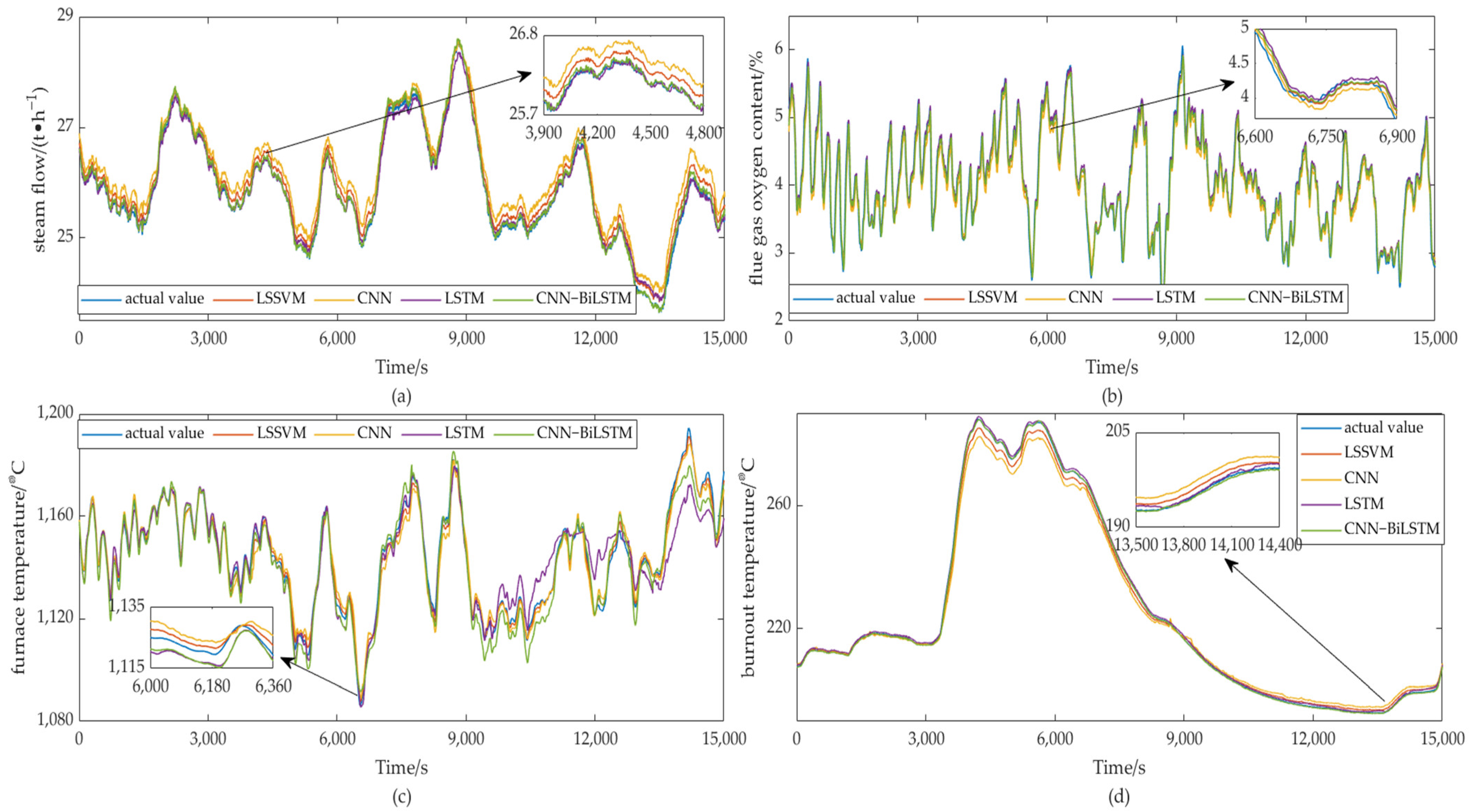
4.2.2. The Influence of Different Models on the Modeling Results

Three classic models, LSSVM, CNN, and LSTM were selected for comparison to verify the effectiveness of the CNN-BiLSTM model. When other conditions were kept the same, the modeling accuracy is as shown in Table 4, and a comparison of the modeling results of the CNN-BiLSTM model is presented in Figure 7.
Table 4 shows that, taking the steam flow as an example, the mean absolute error of LSSVM is 0.178, the mean absolute error of CNN is 0.292, the mean absolute error of LSTM is 0.066, and the mean absolute error of CNN-BiLSTM is 0.051. So, the order of model accuracy from low to high is CNN, LSSVM, LSTM, CNN-BiLSTM. It can be seen that the intelligent model based on deep learning can effectively improve the utility value of the traditional model, and it has stronger generalization ability and modeling accuracy.

5. Conclusions

A combined model based on feature selection and CNN-BiLSTM was constructed in this paper. First, the Lasso algorithm was used to remove invalid and redundant variables from the initial variables to determine the input variables, and the effective feature information was extracted through the CNN network. Finally, the BiLSTM network was used to train the model. Historical operation data from a waste-to-energy plant in the north was used for simulation analysis. The main conclusions are as follows:
(1)
In this paper, based on the historical operation data from waste-to-energy power plants, multi-dimensional feature sets including waste factors, grate operation factors, and air volume factors were used, and high-correlation feature parameters through the effective feature screening of multi-dimensional feature sets by Lasso algorithm were selected. The comparison of before and after feature selection shows that Lasso feature screening for multi-dimensional input feature parameters can improve model accuracy.
(2)
Compared with the traditional LSSVM, CNN, and LSTM models, the bidirectional network model based on feature selection and CNN-BiLSTM selected in this paper, can fully mine data features under multi-dimensional input feature parameters, and it has higher accuracy and applicability.

Author Contributions

Conceptualization, L.C., C.W. and R.Z.; methodology, C.W., R.Z. and J.W.; software, L.C., R.Z. and J.W.; validation, R.Z., C.W. and J.W.; formal analysis, L.C., C.W. and R.Z.; investigation, L.C., R.Z. and J.W.; resources C.W., J.W. and Z.Z.; data curation, L.C., C.W. and R.Z.; writing—original draft preparation, C.W., R.Z. and J.W.; writing—review and editing, L.C., C.W., R.Z., J.W. and Z.Z.; visualization, C.W., R.Z. and J.W.; supervision, L.C., C.W. and R.Z.; project administration, C.W., R.Z. and J.W.; funding acquisition, R.Z. All authors have read and agreed to the published version of the manuscript.

Funding

This research was funded by the Shenzhen Special Sustainable Development Science and Technology Project, grant number KCXFZ20201221173402007.

Institutional Review Board Statement

Not applicable.

Informed Consent Statement

Not applicable.

Data Availability Statement

Not applicable.

Conflicts of Interest

The authors declare no conflict of interest.

References

  1. Chen, S.; Huang, J.; Xiao, T.; Gao, J.; Bai, J.; Luo, W.; Dong, B. Carbon emissions under different domestic waste treatment modes induced by garbage classification. Sci. Total Environ. 2020, 717, 137193. [Google Scholar] [CrossRef] [PubMed]
  2. Moschou, C.E.; Papadimitriou, D.M.; Galliou, F.; Markakis, N.; Papastefanakis, N.; Daskalakis, G.; Sabathianakis, M.; Stathopoulou, E.; Bouki, C.; Daliakopoulos, I.N.; et al. Grocery Waste Compost as an Alternative Hydroponic Growing Medium. Agronomy 2022, 12, 789. [Google Scholar] [CrossRef]
  3. Xu, H. A summary of the development of the municipal solid waste treatment industry in 2017. China’s Environ. Prot. Ind. 2018, 4, 5–9. [Google Scholar]
  4. Huang, M.; He, W.; Incecik, A.; Cichon, A.; Królczyk, G.; Li, Z. Renewable energy storage and sustainable design of hybrid energy powered ships: A case study. J. Energy Storage 2021, 43, 103266. [Google Scholar] [CrossRef]
  5. Sun, G.; Tian, J.; Su, M. The Foundation and Application of Domestic Waste Incineration Power Generation Technology; Hefei University of Technology Press: Hefei, China, 2019. [Google Scholar]
  6. Liu, J. Combustion System Modeling and Optimization Based on Deep Learning; Shanghai Jiaotong University: Shanghai, China, 2016. [Google Scholar]
  7. Sun, Y.; Peng, G.; Jin, K.; Liu, S.; Gardoni, P.; Li, Z. Force/motion transmissibility analysis and parameters optimization of hybrid mechanisms with prescribed workspace. Eng. Anal. Bound. Elem. 2022, 139, 264–277. [Google Scholar] [CrossRef]
  8. Magnanelli, E.; Tranås, O.L.; Carlsson, P.; Mosby, J.; Becidan, M. Dynamic modeling of municipal solid waste incineration. Energy 2020, 209, 118426. [Google Scholar] [CrossRef]
  9. Zhang, Y.; Pan, G.; Zhao, Y.; Li, Q.; Wang, F. Short-term wind speed interval prediction based on artificial intelligence methods and error probability distribution. Energy Convers. Manag. 2020, 224, 113346. [Google Scholar] [CrossRef]
  10. Zhang, Y.; Zhao, Y.; Shen, X.; Zhang, Z. A comprehensive wind speed prediction system based on Monte Carlo and artificial intelligence algorithms. Appl. Energy 2022, 305, 117815. [Google Scholar] [CrossRef]
  11. Peng, D.; Mei, L.; Li, S.; He, J. Research of modeling for the oxygen content of boiler combustion based on large data and neural network. Therm. Power Eng. 2018, 33, 86–92. [Google Scholar]
  12. Song, Q.; Li, Y. Modeling of the boiler combustion system by RBF neural networks. J. Harbin Univ. Sci. Technol. 2016, 21, 89–92. [Google Scholar]
  13. Zhong, Y.; Wei, H.; Yao, W.; Chen, J. Boiler exhaust gas temperature modeling based on particle swarm algorithm and support vector machine. Therm. Power Gener. 2016, 45, 32–36. [Google Scholar]
  14. Duan, Y.; Lv, Y.; Zhang, J.; Zhao, X. Deep learning for control: The state of the art and prospects. Acta Autom. Sin. 2016, 42, 643–654. [Google Scholar]
  15. Hu, H.; Zhang, J.; Liu, H.; Li, M.; Yang, Q. Power plant boiler combustion efficiency modeling approach based on convolutional neural networks. J. Xi’an Jiaotong Univ. 2019, 53, 10–15. [Google Scholar]
  16. Yu, Y.; Han, Z.; Xu, C. NOx concentration prediction based on deep convolution neural network and support vector machine. Chin. Soc. Electr. Eng. 2022, 42, 238–248. [Google Scholar]
  17. Zhang, H. Application of Deep Neural Network in Electric Power Industry Modeling; North China Electric Power University (Beijing): Beijing, China, 2020. [Google Scholar]
  18. Wang, Y.; Xie, D.; Wang, X.; Li, G.; Zhu, M. Prediction of interaction between grid and wind farms based on PCA-LSTM model. Chin. Soc. Electr. Eng. 2019, 39, 4070–4081. [Google Scholar]
  19. Huang, M.; Borzoei, H.; Abdollahi, A.; Li, Z.; Karimipour, A. Effect of concentration and sedimentation on boiling heat transfer coefficient of GNPs-SiO2/deionized water hybrid Nanofluid: An experimental investigation. Int. Commun. Heat Mass Transf. 2021, 122, 105141. [Google Scholar] [CrossRef]
  20. Tibshirani, R.J. Regression Shrinkage and Selection via the LASSO. J. Ro-Yal Stat. Soc. Ser. B Methodol. 1996, 73, 273–282. [Google Scholar] [CrossRef]
  21. Hou, D. Comparative Study and Empirical Analysis of Lasso Type Variable Selection Methods; Shan Dong University: Jinan, China, 2021. [Google Scholar]
  22. Luo, Y.; Fan, Y.; Chen, X. Research on optimization of deep learning algorithm based on convolutional neural network. J. Phys. Conf. Ser. 2021, 1848, 012038. [Google Scholar] [CrossRef]
  23. Burgess, J.; O’Kane, P.; Sezer, S.; Carlin, D. LSTM RNN: Detecting exploit kits using redirection chain sequences. Cybersecurity 2021, 4, 25. [Google Scholar] [CrossRef]
  24. Charu, C. Aggarwal. Neural Networks and Deep Learning; Springer: Cham, Switzerland, 2018. [Google Scholar]
  25. Shen, Q. Study of Dynamic Modeling and Optimization Control Method for Boiler Combustion System; Southeast University: Nanjing, China, 2017. [Google Scholar]
  26. Zhao, Z.; Li, Y.; Yuan, H. Dynamic model for soft sensing of NOx generation in coal-fired units. J. Power Eng. 2020, 40, 523–529. [Google Scholar]
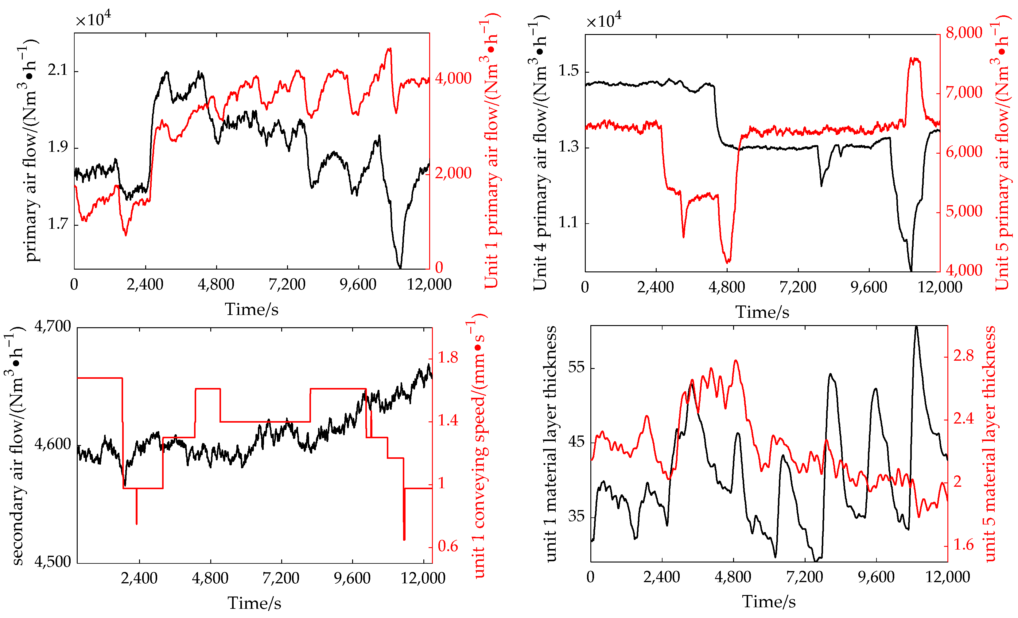
Figure 1. Incinerator structure diagram.
Energies 15 04285 g001
Figure 2. Construction of CNN.
Energies 15 04285 g002
Figure 3. Cyclic unit construction of the LSTM network.
Energies 15 04285 g003
Figure 4. Two-way cyclic neural network expanded by time.
Energies 15 04285 g004
Figure 5. The local trend diagrams of the input variables.
Energies 15 04285 g005
Figure 6. Modeling process diagram.
Energies 15 04285 g006
Figure 7. Modeling result diagram. (a) Comparison of output results of steam flow model; (b) comparison of the output results of the flue gas oxygen content model; (c) comparison of output results of the furnace temperature model; (d) comparison of the output results of the temperature model in the ember stage.
Energies 15 04285 g007
Table 1. Unit and variation range of input variables.
Serial NumberVariable NameUnitVariation Range
1primary air flowNm3/h13,500–23,069
2Unit 1 primary air flowNm3/h299–5932
3Unit 4 primary air flowNm3/h9721–17,763
4Unit 5 primary air flowNm3/h1423–13,173
5secondary air flowNm3/h4538–4673
6unit 1 material layer thickness-11.98–74.25
7unit 5 material layer thickness-1.27–5.05
8unit 1 conveying speed of sliding grate mm/s0.14–2.80
Table 2. Delay time and maximum mutual information of auxiliary variables.
Auxiliary Variable Number12345678
Delay Time2602902409021028070250
Maximum Mutual Information0.77940.69830.84341.08750.93430.72601.28670.7999
Table 3. Evaluation index of the influence of variable selection on modeling results.
Before Variable Selection (MAE/MAPE/RMSE)After Variable Selection (MAE/MAPE/RMSE)
T1 (°C)3.348/0.293/4.2993.245/0.284/4.027
Q (t/h)0.060/0.232/0.0750.051/0.196/0.064
CO2 (%)0.101/2.530/0.1300.100/2.519/0.130
T2 (°C)0.274/0.121/0.4070.240/0.100/0.364
Table 4. Influence of different models on modeling accuracy.
T1 (°C) (MAE/MAPE/RMSE)Q (t/h) (MAE/MAPE/RMSE) C O 2   ( % )   ( MAE / MAPE / RMSE ) T2 (°C) (MAE/MAPE/RMSE)
LSSVM4.226/0.423/5.2390.178/0.654/0.4320.156/3.106/0.1771.324/0.849/1.637
CNN4.540/0.395/6.9410.292/1.140/0.3160.133/3.290/0.1592.198/0.920/2.800
LSTM3.899/0.350/4.3970.066/0.258/0.0870.111/2.637/0.1340.597/0.262/0.652
CNN-BiLSTM3.245/0.284/4.0270.051/0.196/0.0640.100/2.519/0.1300.240/0.100/0.364
Publisher’s Note: MDPI stays neutral with regard to jurisdictional claims in published maps and institutional affiliations.

