Fuzzy Logic and Linear Programming-Based Power Grid-Enhanced Economical Dispatch for Sustainable and Stable Grid Operation in Eastern Mexico

Abstract

Sustainable, stable, and cost-optimized operation of power grids must be the main objectives of power grid operators and electric utilities. The energy transition towards a preponderant green energy economy requires innovative solutions to enhance the power grid economic dispatches looking for a better allocation of the energy demand among the diverse renewable and fossil fuel energy plants. Green renewable energy systems must be preferred over fossil fuel generators when they are available. However, fossil plants are still required to be kept operational due to the variability and uncertainty of renewable energy plants. This study proposes a hybrid rational economic dispatch model that combines a cost minimization linear model enhanced with a fuzzy logic system for decision-making on wind and hydropower minimum and maximum generation levels. The model considers the intermittency of wind energy and recognizes the strategic value of hydropower as energy storage. The results of the model with real data taken from wind, hydroelectric, geothermal, nuclear, bioenergy, and fossil fuel power plants in the eastern region of Mexico show that a fairer, rational, and cost-optimized power grid economic dispatch can be achieved with the proposed approach.

1. Introduction

Achieving net-zero emissions goals requires decarbonizing the electricity generation system with the greater participation of clean and renewable energy sources while maintaining its reliability, economics, and efficiency [1,2]. However, one of the main barriers that slows down a greater penetration of renewable energies is their high variability and intermittency, putting at risk the reliability and security of the electricity grid [3]. Furthermore, the high variability and uncertainty of renewables cause the need to have costly energy storage systems or fossil fuel plants as backup systems, with the associated high costs. In addition, it creates a tremendous operational challenge because constant energy generators must be frequently adjusted to match the demand and the dynamic variation of renewables [4]. Therefore, this work aims to develop a new management model for electricity generation networks that maximize the participation of renewables but in a context that protects the operational response of baseload plants and ensures the reliability and cost-effectiveness of the power system.

The objective of the electric utility or grid operator is to minimize the total generation cost of meeting the electricity demand. Economic dispatch (ED) is how the utility operator selects which of its generators will be used to meet electricity demand [5]. With the proliferation of renewable energies and the interest in increasing their use due to sustainability goals, it is necessary to enhance the current economic dispatches model to consider the approach to cost minimization in addition to other factors, such as the intermittence in renewable power generation or the advantage of the energy storage capability of hydropower plants. Furthermore, a power generation network is more productive when plants of different technologies have an ED to optimize natural and financial resources [6,7,8,9]. Optimal power dispatches of multisource systems have been demonstrated for the control of distributed generation systems for smart grids, including photovoltaic (PV) panels, wind turbines (WTs), battery energy storage systems (BESSs), and electric vehicles (EVs) [10].

Soft computing is based on techniques such as fuzzy logic (FL), genetic algorithms, artificial neural networks, machine learning, and expert systems. Since their introduction, soft computing methods have been a significant research area to solve control and optimization problems. In the literature, there is a wide diversity of methods and algorithms proposed for the optimization of energy grids, such as linear programming [11], quadratic programming [12], genetic algorithms [13], Taboo search [14], optimal control [15], and particle swarm algorithm [16]. However, some of the drawbacks of these algorithms are that they offer only local and not absolute optimal results, that is, optimal solutions that are not necessarily the most efficient. On the other hand, the fuzzy logic strategy has become an attractive decision-making tool for energy management [17,18]. For example, it has been used to calculate the risk associated with variations in costs [19] or to predict wind power generation [20].

Regarding ED, fuzzy logic has been used with other soft computing methods. Previous works have demonstrated the capability of decision trees combined with FL in solving optimization problems for the ED, including environmental constraints and by adding fuzzy logic to the unit operational limits and loads [21]. Genetic algorithm techniques have also been combined with FL in a genetic-fuzzy-based approach for solving ED problems [22,23]. FL has also been incorporated into the particle swarm optimization algorithm to solve non-smooth and constrained economic dispatch [24,25]. FL is an efficient tool for dealing with multiple tasks instead of having a precise model to deal with each task individually [26]. FL can also predict the wind velocity, solar radiation, and load consumption, or even the status of the grid [27]. Some previous works have addressed the problem of optimal power dispatch in a system with different power sources, using fuzzy logic control to manage the power flow between different sources under variable demands [10,28]. However, these studies were conducted at a microgrid scale, so studies with power plant networks with real operating parameters are still needed.

This work presents an ED model incorporating fuzzy inference systems (FISs) to establish minimum and maximum operational limits of power generation for wind and hydropower plants in the eastern region of Mexico. The novel FL scheme allows for partially restricting wind power generation as a function of its present and forecast availability and compensates it with the energy storage capacity of the hydroelectric plants. The results can be used with a previously developed ED model to obtain an enhanced economic dispatch that can be regarded as a hybrid rational economic dispatch. The paper is organized as follows: Section 2 describes the general scheme for the fuzzy logic decision-making strategy and the adapted model for economic dispatch. The results and their discussion are presented in Section 3 and Section 4, respectively. Section 5 presents the conclusions.

2. Materials and Methods

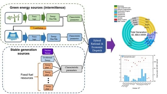
2.1. General Model

The proposed general model is to apply fuzzy logic inference systems for the decision-making process of selecting maximum and minimum operating levels of the wind power generators and to partially compensate for their intermittence with energy contribution from hydroelectric power plants. The combined power generation of wind and hydraulic power plants is then considered with the other conventional power plants in the optimal power dispatch. Therefore, the analyzed energy network in this work was divided into two main groups: variable and constant generation power plants (Figure 1). In this scheme, a group of plants with a variable resource, such as wind power plants (WPP) and hydropower plants (HPP), is presented, whose operating mechanisms and power generation are a function of fluctuating parameters, such as wind speed or the water level in a dam. For the second classification, plants are stable in terms of energy generation. This group includes fossil fuel, geothermal, bioenergy, and nuclear power plants. It is important to note that, for the latter group, their operation and characteristic output parameters are stable, so they do not require extraordinary modeling.

In contrast, for the set of intermittent and uncertain power sources, an FL scheme is proposed to have intermediate values of the output energy generation of each plant between two states. The purpose is to limit the participation of renewables based on the variability and intermittency they have accumulated in the current step and the forecast availability for the next step. In this way, the aim is to qualify their intermittency. Once the parameters of each plant that form the network were defined, the equations describing the energy system were established, which are the input data for the economic dispatch model. Finally, the conditions to achieve the minimization of costs of the complete system were obtained.

2.1.1. Modeling of Wind Energy Plants

The modeling approach for the energy output of a WPP is based on a fuzzy logic description, as shown in Figure 2. The starting point is to consider a wind power plant i = 1 and assume that its operation depends on the average wind speed measured in the current period step and the forecast for the next step for which the wind power generation participation is estimated (see Figure 2a). With this rule, even if the wind speed forecast is favorable but has high intermittency in the present step, its power generation is limited in the next step. This is a strategy to penalize its variability. The wind plant can access a higher power generation level if the forecast is favorable and its availability is adequate in the current step.

Stage 1. Due to the dynamic nature of the wind and the range of speeds in which it oscillates, linguistic variables associated with sub-ranges are established for the current measured wind velocity (see

Table 1. Wind classification.

Type of Wind	Minimum Speed m/s	Maximum Speed m/s
Calm	0	0.4
Light Air	0.5	1.5
Light Breeze	1.6	3.4
Gentle Breeze	3.5	5.5
Moderate Breeze	5.5	8
Fresh Breeze	8.1	10.9
Strong gale	11.4	13.9
Fresh Breeze	14.1	16.9
Fresh gale	17.4	20.4
Stong gale	20.5	23.9
Whole gale	24.4	28
Storm	28.4	32.5
Hurricane	32.6	-

). This process of generating subsets is called fuzzification. A similar procedure is performed concerning the forecast wind availability estimated with a probability function. From these estimations, another subset of possible velocity ranges is generated. The wind forecast for the day is established through the Weibull probability function [29].

Stage 2. The next step is to establish the inference rules for the fuzzy system, which are a group of rules between both sets.

Stage 3. The last step of the process is called defuzzification and consists essentially of giving a numerical value to the resulting membership function. This generates two characteristic output system parameters: the maximum and minimum generation energies (E_wmax and E_wmin, respectively). The whole FL process described above is applied to each wind plant that makes up the system (i = 1, 2, 3…n).

The wind speed range in which the plants operate was obtained, as shown in Table 1 [30], and they were regrouped in terms of linguistic variables, defined in

Table 2. Fuzzification of the current wind speed.

Fuzzification	Range [m/s]
Null	[0–3.4]
Low	[3.5–8]
Medium	[8.1–10.9]
High	[11–23.9]
Stop	[24–-]

, to carry out the fuzzification process of Stage 1.

The indicated linguistic variables generate the membership functions scaled in a range of 0–1 [31]; the input values of the current wind speed and wind speed forecast for each wind power plant are shown in Table S1 of the Supplementary Materials. Figure 3 shows the membership functions of the fuzzy sets of the wind speed for the values in Table 2.

Then, a group of inference rules characterizes the performance of the fuzzy system. (Stage 2). The rules defined for the wind system are set out in Figure 4.

Subsequently, the inference process of the fuzzy logic methodology is responsible for calculating the result obtained from the input values using the membership functions described in Figure 5. This defuzzification process generates the minimum and maximum energy of each plant, shown in Figure 5 (Stage 3). The values obtained in each WPP are shown in Table S2 of the Supplementary Materials.

2.1.2. Modeling of Hydraulic Power Plants

The process described above applies similarly to hydraulic power plants. HPPs also have a variable operation defined by the height levels or volume of water within the dam (see Figure 2b). Additionally, recognizing its strategic value as a storage energy system, a water storage capacity of 60% was fixed, so that if the dam is below this fill level, the power production stops. The height up to this value was one of the variables that makes up the input fuzzy system. The other parameter was the sum of the maximum energy contributions of each wind power plant mentioned above (see Figure 2b). The objective is that if the production of renewable sources—wind power, in this case—is low, and water levels are high, the generation of hydropower can be increased, performing as a backup system. This creates a synergy between the renewables and hydropower to ensure a more significant proportion of clean energy in the generation matrix.

The level or volume of water in the dam is one of the input variables to the hydroelectric fuzzy system, as shown in Figure 2b. For our case study, the height of the water was assumed from real data obtained by [32], and the possible water level values for each hydropower plant were related to linguistic variables through ranges, as shown in

Table 3. Fuzzification of water height.

Fuzzification	Water Height (m)
Null	(0–3.4)
Low	(3.5–8)
Medium	(8.1–10.9)
High	(11–23.9)
Stop	(24–-)

.

These values were used to establish the membership functions for one hydroelectric power plant, as shown in Figure 6.

It is important to note that the membership ranges are different according to the particular elevation characteristics of each HPP established. These input parameters of hydro plants are found in Table S3 of the Supplementary Materials. In the present work, HPPs were assumed as support and energy storage systems for renewables. We propose that in regions where water resources are abundant, as in the case of eastern Mexico, hydropower should be managed as a storage source. Therefore, in the fuzzy logic model for HPPs, the power generation is a function of two parameters: (a) the water level in the dam and (b) the total contribution of the wind power plants. This means that if the energy production of the WPPs is low, the model will seek to increase the hydro output to compensate for the drop in renewables; see Figure 2b. The membership functions of the wind input variable are shown in Figure 7.

Using the input variables, the rules of the hydropower fuzzy system described in Figure 8 were established.

Finally, the inference rules generated the values of maximum and minimum energy produced by HPPs, as shown in Figure 9; these obtained values are found in Table S4 of the Supplementary Materials.

As can be seen, both fuzzy systems are coupled, establishing the characteristic parameters of the different wind and hydropower plants under study. These ranges of maximum and minimum energy for each type of plant are necessary as input data to the economic dispatch model, which is in charge of searching for optimized system conditions (see Figure 2).

2.1.3. Economic Dispatch

The ED was implemented in this work through a linear programming model, a detailed description of the model is already reported elsewhere [29]. The analytical model of economic dispatch is formulated as follows.

The electric generation network is integrated by j = 1, 2, 3, … J plants, each with its own particular characteristics, where J is the total number of generation plants in the system, and each j works under the maximum and minimum limits given by the following:

$$P_{min, j}·v_j \le P_j\le P_{max,j}·v_j$$

(1)

where $P_j$ is the power generated by each plant j; $Pmi{n}_j, Pma{x}_j$ are the minimum and maximum powers of each plant, and $v_j$ is a binary variable indicating when the plant is working. The power generated by each plant must satisfy the demand D requested by the electrical distribution network; therefore,

$$D={\displaystyle \sum }_{j=1}^J{P}_j$$

(2)

In addition, demand fulfillment generates costs for each plant, whose total cost of generation is called R. Thus, the cost function R is expressed as follows:

$$R={\displaystyle \sum }_{j=1}^J\left(A_j·v_j+B_j·p_j +M_j·z_j\right)$$

(3)

where A_j indicates the fixed cost of the plant, B_j is the variable cost of production, pj is the plant production, M_j is the cost of stopping each plant, and z_j is a binary shutdown variable. For the scheduling of plants by periods, three parameters must be considered for planning: (a) the starting plant; (b) the stopping plant; (c) the allocation of energy to be generated. Furthermore, these three parameters must satisfy the demand in each time cycle. In such a case, the planning horizons are divided into a day by k time cycles and meeting k = 1,2, …, K, where K is the total number of cycles established for the study. Based on the above, the objective function cost minimization R is now rewritten at all time intervals as follows:

$$R={\displaystyle \sum }_{k=1}^K{\displaystyle \sum }_{j=1}^J((A_j+B_j)·E_{jk}+C_j·y_{jk} +M_j·z_{jk})$$

(4)

where the sum of all plant costs in each of the periods is represented. The first term of Equation (4) incorporates the fixed cost A_j and the variable cost Bj of each generation plant, which are based on the generation carried out, with these multiplied by the energy Ejk to be generated in each generation plant j in period k. The term Cj indicates the startup cost of a plant that is incurred at the time the plant is started up. Finally, the equation incorporates the cost M_j, generated when a plant is off. Thus, each of the costs described is set according to the binary state parameters of activation or shutdown, called v_jk, y_jk, and z_jk, respectively.

The constraints established to satisfy the different energy demands while optimizing the use of the available resources and minimizing the total generation cost are outlined in Equations (4)–(12). Therefore, each plant cannot generate more or less energy than its operating limits (Equations (5) and (6)). The change in the generation between periods cannot rise or fall above the maximum ramps up or down for each plant (Equations (7) and (8)). Binary variables allow for establishing when a plant is in operation in the previous period, and in the following period, it cannot start up because it was already started up (Equation (9)). In addition, it cannot be in operation and turned off at the same time, as shown in Equation (10), the state logic of Equation (11) shows the behavior of the binary variables of operation, start, and stop. The model satisfies the demands established in the different periods due to Equation (12). The model equations are presented as follows [29]:

Minimum energy:

$$E_{min,j}·v_{jk}\le E_{jk}$$

(5)

Maximum energy:

$$E_{jk}\le E_{max,j}·v_{jk}$$

(6)

Maximum load rise ramp:

$$E_{jk+1}-E_{jk}\le U_j$$

(7)

Maximum load descent ramp:

$$E_{jk}-E_{jk+1}\le F_j$$

(8)

Start:

$$v_{jk}-v_{jk-1}\le y_{jk}$$

(9)

On/Stop:

$$v_{jk}+z_{jk}=1$$

(10)

State:

$$v_{jk}-v_{jk-1}+y_{jk}-z_{jk}\le 0$$

(11)

Demand:

$$D_k={\displaystyle \sum }_{j=1}^J{E}_{jk}$$

(12)

The parameters of each plant, such as maximum energy ($E_{max,j}$), minimum energy ($E_{min,j}$), variable costs $\left(B_j\right),$ fixed costs $\left(A_j\right)$, startup costs $\left(C_j\right),$ and shutdown costs ($M_j$), are presented in Table S5 of the Supplementary Materials.

2.2. Case of Study: Eastern Mexico Zone

The case study was located in Mexico, where the energy distribution system is formed by nine zones [33], as shown in Figure 10. In particular, the interest in applying the hybrid economic dispatch model was focused on the eastern zone, which has 110 generation plants and a significant and diverse mix of generation technologies. It is worth mentioning that the zone has a remarkable importance because it represents 22% of the total national demand [33] and contributes to adjacent zones. To simplify the analysis of the proposed model, a significant sample of 17 of the 110 plants installed in the eastern zone was selected. Figure 10 shows the geographic distribution of the sample.

Additionally, Figure 11 describes the distribution of installed power according to the type of technology located in the eastern zone and the study sample of the 17 plants considered. Let us note that the selected sample is representative.

Finally, for comparative purposes to evaluate the model’s performance under annual dynamic conditions, such as demand variation, wind resource availability, and water levels; four days were arbitrarily chosen, one for each of the four seasons. Figure 12 shows the variation of demand (MW) as a function of the time of day for four days selected. As can be seen, the demand tended to decrease during the first hours of the day, from 12:00 to 6:00 a.m. It then began to increase during the course of the day until it reached a maximum in the evening from 6:00 p.m. to 12:00 a.m. It can also be observed that the demand was lower on the winter day than on the summer and autumn days. The bar chart represents the demand transformation into consumption (MWh) in 6-h time periods (1 period). These values are the input data for the model. It must find the most optimal generation matrix to satisfy the demand considering the availability of wind and hydro resources. Hydropower is used as a backup source to compensate for the variability of wind power. The ED optimization considers the fixed and variable costs and the plants’ ramp-up and -down costs, established in Equation (4), and subject to the restrictions of Equations (5)–(12) implemented in Matlab^® through the mixed-integer linear programming function intlinprog to obtain the results.

3. Results

3.1. Electricity Generation Matrix

The optimization model results for the eastern region of Mexico can be seen in Figure 13, which shows the electrical generation matrix by technology for the four periods on four different days of the year. The innermost ring represents the first period, which corresponds to 12:00 a.m. to 6:00 a.m., while the last period, from 6:00 p.m. to 12:00 a.m., is the outermost ring.

Figure 13 shows the generation matrix of (a) a winter day (15 January), where electricity generation during the first period was 18, 695.6 MWh, and the source with the highest percentage of generation was hydropower with 57.7%. The next most significant source was the gas combined cycle, with 30%. The rest of Period 1’s consumption was supplied by wind power, at 12.4%. As the day went on, the demand increased in Periods 2, 3, and 4, Figure 12. Generation increased from 20.38 GWh in Period 2 to 22.93 GWh in Period 4, as shown in

Table 4. Electricity generation by period on the four studied seasonal days.

	15 January (MWh)	15 April (MWh)	15 June (MWh)	15 October (MWh)
Period 1	18,695.8	21,065.0	22,882.0	21,951.8
Period 2	20,382.4	21,158.3	21,750.6	21,670.1
Period 3	21,866.9	22,973.4	23,399.2	23,191.4
Period 4	22,937.5	24,612.3	24,853.8	25,081.4
Total	83,882.6	89,809.0	92,885.6	91,894.7

. Hydropower participation increased by 61.2%, 63.8%, and 65.5%, respectively. The increase in hydropower generation was due to higher demand and the physical limitations of the installed capacity of the combined cycle and wind power. (b) For the spring day (15 April), there was an increase in consumption of 7% compared to 15 January, from 83.9 GWh to 89.8 GWh. The consumption increment in the first two periods of the day was supplied by incorporating cogeneration (6.7%) and steam turbines (2.5%); together they accounted for 9.2% (1.93 GWh) of the 21 GWh required in Period 1, meaning an average increase in demand of 322 MW. However, as can be seen in Figure 12, the demand and consumption increased even more for the last two periods of the day, so greater participation of steam thermoelectrics was needed, and the startup of small geothermal, combustion engine, and bioenergy plants was also required. (c) The summer day (15 June) was the day with the highest consumption of all four days. For Period 1, the consumption reached almost 23 GWh, but in contrast, the participation of hydro and wind power was reduced. This generated a larger energy deficit, which was solved with the startup of the nuclear plant. It is important to note that although nuclear energy has lower costs than steam thermoelectric power due to its size (1510 MW), it is not recommended to enter into operation when the energy deficit is small. Generation was mainly defined by hydropower, nuclear, combined cycle, cogeneration, and wind. These maintained approximately stable production throughout the day. However, there was a slight difference in Period 4; consumption increased to 24.85 GWh, and the energy deficit was covered by a greater share of cogeneration, from 6.2% in the first period to 8.6% in the last. (d) On the fall day (15 October), hydropower had the lowest participation of the four days. The low output of the hydro plants, below 47.8% in Period 1, led to the higher participation of nuclear generation. Although the consumption between 15 April (21 GWh) and 15 October (21.95 GWh) was close, the high deficit caused by the reduction in hydropower gave rise to the startup of the operation of nuclear energy. The highest consumption in the four days analyzed was present in the last period of the fall day, at 25.08 GWh; therefore, a greater participation of the nuclear plant and the entry into operation of the geothermal power plant are required. As can be seen from these results, the dispatch model takes into account the fixed and variable costs of the different plants and considers the changes in demand, the size of each plant, and the startup and shutdown costs.

Table 4 summarizes the electricity generated in each period for the four different season days and the total generation for each day. The energy generated by each plant during the four periods for the four days of the study is reported in Tables S6–S9 of the Supplementary Materials.

The high participation of hydropower plants in the electricity matrix of eastern Mexico is due to the particular conditions of the study area, which has the highest concentration of hydroelectric install capacity in Mexico due to the abundant rainfall in the region.

3.2. Electricity Cost by Plant

Each of the 17 plants has a cost, regardless of whether it is in operation or remains out of operation. The variable costs of plants that require fuel increase as their energy production increases. All plants have fixed costs.

Figure 14 shows the results of the costs of each of the 17 plants during Period 4. The bar graph represents the electricity generated by each plant and the red dots represent the cost of the plant in USD during the period. (a) As can be seen, the energy generated on 15 January was mostly from combined cycle and hydropower plants, representing the highest costs of approximately USD 800,000 and USD 200,000, respectively, during the period. However, if we calculate the cost per unit in USD per megawatt hour, the average cost for CC was USD 71.5/MWh and USD 72.9/MWh for hydro. The lowest-cost technology was wind power, at USD 67.6/MWh. (b) On the spring day (15 April), the demand was higher, and the production of the hydroelectric plants was lower. Therefore, this energy deficiency was covered by steam turbine, combustion engine, and geothermal production. As can be seen, hydro was the most expensive technology during the period, exceeding USD 500,000. However, the most costly plant per unit was a steam turbine at USD 108/MWh. (c) On the summer day, 15 June, the consumption was the highest at 92.8 GWh. Hydro, combined cycle, nuclear, and wind power production were the main generators. The most costly plant of the period was the hydroelectric plant III, with a total cost of USD 415,000. However, in terms of the cost per unit, the most expensive were combustion engine, geothermal, and nuclear production, with USD 144, 97, and 91.6 per megawatt hour. In addition, it should be clarified that the geothermal and combustion production were minimal. (d) The autumn day was very similar to the summer day. The highest cost was hydro III at USD 400,000. The total costs and total energy generated by each plant during the four periods for the four days of the study are reported in Tables S6–S9 of the Supplementary Materials.

Although the unit costs per technology are different, the optimization model helps us choose the cheapest technology according to the demand variation. The most critical cost parameter is the average cost per unit of energy in each period. In Figure 15, the unit cost per period is illustrated. This value was obtained by dividing all the energy produced during the period by the sum of the costs of all the plants, whether or not they were in operation. This gave an average price of the energy generated. As can be seen in the figure, the lowest costs were achieved on the winter day (15 January). There was low demand, which could be supplied with the installed capacity of the cheapest technologies—wind, combined cycle, and hydro. In the first period of the different days, the cost per unit was lower on the spring day than on the summer and autumn days. However, the demand increased in the last period of the day. Meanwhile, in summer, it was supplied with an increase in hydropower generation, allowing for keeping the unit cost stable; for the spring and autumn days, the hydro could not increase. Therefore, the energy deficit had to be supplied with more expensive technologies, such as nuclear and steam turbines.

4. Discussion

Sustainable energy policies have established that green energies must be preferred over fossil fuel generators when they are available, but fossil plants are still required to be kept operational due to the intermittence of wind, solar, hydroelectric, and other renewable energy plants. In the presented enhanced economic dispatch, the operational levels for the wind generation plants are selected by a fuzzy inference system with combined inputs of actual wind and the short-term wind forecast. The total amount of energy contribution by all of the wind generators is put into another fuzzy inference system that also considers the actual volume of each hydroelectric generator to define the minimum and maximum power generation levels of the individual hydroelectric plant. The main results of the proposed approach are the following:

• The intermittence of the wind generator is compensated for with the hydroelectric plants as long as they have enough capacity. In this way, the energy storage capacity of the hydroelectric plants is used to supply the energy generated by renewable energy sources.
• The remaining energy generation capacity to supply the total energy demand is distributed among the fossil fuel plants. This implies that some energy is generated by the thermoelectric plants to keep them operational and profitable.
• Once a fuzzy logic adjustment has been made to wind power based on its intermittency and a minimum reserve level of hydroelectric power is ensured, the model tries to satisfy the current demand with the cheapest technologies, taking into account the costs of turning a plant on and off. The increase in demand on a spring day is supplied with a gas turbine thermoelectric plant, which has a higher unit cost than nuclear. However, it is feasible to turn on the nuclear plant for the summer and autumn days when the consumption levels are higher.

The proposed enhanced economical dispatch implies better power grid stability and fair allocation of the energy demand among the diverse renewable energy and fossil fuel plants.

5. Conclusions

Economic dispatch (ED) implies the cost-effective distribution of the total energy demand among the diverse available types of green energy sources and the installed capacity of fossil fuel power generation. This study proposed a hybrid rational economic dispatch that combines a linear model for cost minimization that is enhanced with a fuzzy logic system for the decision-making of the minimum and maximum operational levels of the wind generation and hydroelectric plants. The intermittence of the wind generator is compensated for with the hydroelectric plants as long as they have enough capacity. The remaining energy generation capacity is distributed among the fossil fuel plants. This implies better distribution of the power generation among the power generation plants. The results of the model with real data taken from wind, hydroelectric, geothermal, nuclear, bioenergy, and fossil fuel power plants in the southeastern region of Mexico show that a fairer, rational, and cost-optimized power grid economic dispatch can be achieved with the proposed approach. In all weather seasons, the hydropower generation tended to compensate for the wind generator, but there were mixed results on the spring and autumn days due to higher energy demand and lower availability of water (average of 53% of the power was generated by hydro plants versus 9.4% by wind power). The expected compensation by hydropower was more clearly seen in January, as demand increased with the time of day and the share of wind decreased from 12.4% to 10.1%. This decrease was offset by an increase in hydroelectric generation, which went from 55.7% to 65.5%. On the summer day, the effect was similar; the demand increased with the passing of the day, and therefore, the share of wind power decreased from 8.4 to 7.7%. Hydro remained stable at 51%, although, in net terms, it increased its production due to the fact that demand was higher in the evening. The deficit was covered by fossil fuel and nuclear plants. On the spring and autumn days, the reduction in the share of wind was not accompanied by an increase in hydro due to its water levels, so the shortfall, in this case, was covered by geothermal, nuclear, and fossil fuel production.

References

1. Cantarero, M.M.V. Of renewable energy, energy democracy, and sustainable development: A roadmap to accelerate the energy transition in developing countries. Energy Res. Soc. Sci. 2020, 70, 101716. [Google Scholar] [CrossRef]
2. Schleussner, C.F.; Rogelj, J.; Schaeffer, M.; Lissner, T.; Licker, R.; Fischer, E.; Knutti, R.; Levermann, A.; Frieler, K.; Hare, W. Science and policy characteristics of the Paris Agreement temperature goal. Nat. Clim. Chang. 2016, 6, 827–835. [Google Scholar] [CrossRef] [Green Version]
3. Ayodele, T.R.; Ogunjuyigbe, A.S.O. Mitigation of wind power intermittency: Storage technology approach. Renew. Sustain. Energy Rev. 2015, 44, 447–456. [Google Scholar] [CrossRef]
4. Moretti, M.; Njakou Djomo, S.; Azadi, H.; May, K.; De Vos, K.; Van Passel, S.; Witters, N. A systematic review of environmental and economic impacts of smart grids. Renew. Sustain. Energy Rev. 2017, 68, 888–898. [Google Scholar] [CrossRef]
5. He, L.; Lu, Z.; Geng, L.; Zhang, J.; Li, X.; Guo, X. Environmental economic dispatch of integrated regional energy system considering integrated demand response. Int. J. Electr. Power Energy Syst. 2020, 116, 105525. [Google Scholar] [CrossRef]
6. Ahmadi, P.; Dincer, I. 5.9 Optimization in Energy Management. In Comprehensive Energy Systems; Ibrahim, D., Ed.; Elsevier: Amsterdam, The Netherlands, 2018; Volume 5, pp. 351–388. [Google Scholar] [CrossRef]
7. Suganthi, L.; Samuel, A.A. Energy models for demand forecasting—A review. Renew. Sustain. Energy Rev. 2012, 16, 1223–1240. [Google Scholar] [CrossRef]
8. Yue, X.; Pye, S.; DeCarolis, J.; Li, F.; Rogan, F.; Gallachóir, B. A review of approaches to uncertainty assessment in energy system optimization models. Energy Strategy Rev. 2018, 21, 204–217. [Google Scholar] [CrossRef]
9. Mayer, M.J.; Szilágyi, A.; Gróf, G. Environmental and economic multi-objective optimization of a household level hybrid renewable energy system by genetic algorithm. Appl. Energy 2020, 269, 115058. [Google Scholar] [CrossRef]
10. Fotopoulou, M.; Rakopoulos, D.; Blanas, O. Day, Ahead Optimal Dispatch Schedule in a Smart Grid Containing Distributed Energy Resources and Electric Vehicles. Sensors 2021, 21, 7295. [Google Scholar] [CrossRef]
11. Di Pilla, L.; Desogus, G.; Mura, S.; Ricciu, R.; Di Francesco, M. Optimizing the distribution of Italian building energy retrofit incentives with Linear Programming. Energy Build. 2016, 112, 21–27. [Google Scholar] [CrossRef]
12. McLarty, D.; Panossian, N.; Jabbari, F.; Traverso, A. Dynamic economic dispatch using complementary quadratic programming. Energy 2019, 166, 755–764. [Google Scholar] [CrossRef]
13. Arabali, A.; Ghofrani, M.; Etezadi-Amoli, M.; Fadali, M.; Baghzouz, Y. Genetic-Algorithm-Based Optimization Approach for Energy Management. IEEE Trans. Power Deliv. 2013, 28, 162–170. [Google Scholar] [CrossRef]
14. Kawaguchi, S.; Fukuyama, Y. Reactive Tabu Search for Job-shop scheduling problems considering peak shift of electric power energy consumption. In Proceedings of the IEEE Region 10 Conference (TENCON). Marina Bay Sands, Singapore, 22–25 November 2016. [Google Scholar] [CrossRef]
15. Killian, M.; Zauner, M.; Kozek, M. Comprehensive smart home energy management system using mixed-integer quadratic-programming. Appl. Energy 2018, 222, 662–672. [Google Scholar] [CrossRef]
16. Rodzin, S.I. Smart dispatching and metaheuristic swarm flow algorithm. J. Comput. Syst. Sci. Int. 2014, 53, 109–115. [Google Scholar] [CrossRef]
17. McBratney, A.B.; Odeh, I.O.A. Application of fuzzy sets in soil science: Fuzzy logic, fuzzy measurements, and fuzzy decisions. Geoderma 1997, 77, 85–113. [Google Scholar] [CrossRef]
18. Vojtáš, P. Fuzzy logic programming. Fuzzy Sets Syst. 2001, 124, 361–370. [Google Scholar] [CrossRef]
19. Kumar, R.; Chauhan, A.; Aggarwal, A. Devising a new technique for all-thermal economic dispatch problem’s solution employing angular fuzzy sets and variation factor. In Proceedings of the Communication, Control and Intelligent Systems (CCIS 2015), Mathura, India, 7–8 November 2015. [Google Scholar] [CrossRef]
20. Miranda, V.; Hang, P.S. Economic dispatch model with fuzzy wind constraints and attitudes of dispatchers. IEEE Trans. Power Syst. 2005, 20, 2143–2145. [Google Scholar] [CrossRef] [Green Version]
21. Roa-Sepulveda, C.A.; Herrera, M.; Pavez-Lazo, B.; Knight, U.G.; Coonick, A.H. Economic dispatch using fuzzy decision trees. Electr. Power Syst. Res. 2003, 66, 115–122. [Google Scholar] [CrossRef]
22. Song, Y.H.; Wang, G.S.; Wang, P.Y.; Johns, A.T. Environmental/economic dispatch using fuzzy logic controlled genetic algorithms. IEEE Proc.-Gener. Transm. Distrib. 1997, 144, 377–382. [Google Scholar] [CrossRef]
23. Nasiruzzaman, A.B.M.; Rabbani, M.G. Implementation of Genetic Algorithm and fuzzy logic in economic dispatch problem. In Proceedings of the International Conference on Electrical and Computer Engineering, Dhaka, Bangladesh, 20–22 December 2008. [Google Scholar] [CrossRef]
24. Niknam, T.; Mojarrad, H.D.; Nayeripour, M. A new fuzzy adaptive particle swarm optimization for non-smooth economic dispatch. Energy 2010, 35, 1764–1778. [Google Scholar] [CrossRef]
25. Somasundaram, P.; Swaroopan, N.J. Fuzzified Particle Swarm Optimization Algorithm for Multi-area Security Constrained Economic Dispatch. Electr. Power Comp. Syst. 2011, 39, 979–990. [Google Scholar] [CrossRef]
26. Al-Sakkaf, S.; Kassas, M.; Khalid, M.; Abido, M.A. An energy management system for residential autonomous DC microgrid using optimized fuzzy logic controller considering economic dispatch. Energies 2019, 12, 1457. [Google Scholar] [CrossRef] [Green Version]
27. Hetzer, J.; David, C.Y.; Bhattarai, K. An economic dispatch model incorporating wind power. IEEE Trans. Energy Convers. 2008, 23, 603–611. [Google Scholar] [CrossRef]
28. Meje, K.; Bokopane, L.; Kusakana, K.; Siti, M. Optimal power dispatch in a multisource system using fuzzy logic control. Energy Rep. 2020, 6, 1443–1449. [Google Scholar] [CrossRef]
29. López, E.; Domínguez-Cruz, R.F.; Salgado-Tránsito, I. Optimization of Power Generation Grids: A Case of Study in Eastern Mexico. Math. Comput. Appl. 2021, 26, 46. [Google Scholar] [CrossRef]
30. The Royal Meteorological Society. The Beaufort Scale. Available online: https://www.rmets.org/metmatters/beaufort-scale (accessed on 2 March 2022).
31. Precup, R.E.; Hellendoorn, H. A survey on industrial applications of fuzzy control. Comp. Ind. 2011, 62, 213–226. [Google Scholar] [CrossRef]
32. García-Gutiérrez, H.; Nava-Mastache, A. Selección y Dimensionamiento de Turbinas Hidráulicas para Centrales Hidroeléctricas, 1st ed.; Universidad Nacional Autónoma de México, Facultad de Ingeniería, Cuidad de México: Ciudad de México, México, 2013; pp. 56–82. [Google Scholar]
33. Centro Nacional de Control de Energía (CENACE México). Demandas del Sistema Eléctrico Nacional. Available online: https://www.cenace.gob.mx/Paginas/Publicas/Info/DemandaRegional.aspx (accessed on 2 March 2022).
Figure 1. Optimization of a power generation network based on FL and linear system models. The network is composed of plants operating with variable and constant supply sources.
Energies 15 04069 g001
Figure 2. Power generation modeling based on FL methodology for (a) wind power plants; (b) hydroelectric power plants.
Energies 15 04069 g002
Figure 3. Membership functions of the wind speed input variable of the wind power plants belonging to the sample of the eastern region. X-axis range in (m/s).
Energies 15 04069 g003
Figure 4. Inference rules of the wind fuzzy system (Stage 2).
Energies 15 04069 g004
Figure 5. Membership functions of the output variables of wind power plants obtained from the defuzzification process. (a) Minimum energy to be generated; (b) maximum energy to be generated (Stage 3). X-axis range in (MWh).
Energies 15 04069 g005
Figure 6. Membership functions of the input variable height of the hydraulic fuzzy system. X-axis range in (m).
Energies 15 04069 g006
Figure 7. Membership functions of the wind power input variable to the hydraulic fuzzy system. X-axis range in (MWh).
Energies 15 04069 g007
Figure 8. Inference rules of the hydropower fuzzy system.
Energies 15 04069 g008
Figure 9. Membership functions of the output variables of hydroelectric power plants obtained from the defuzzification process. (a) Minimum energy to be generated; (b) maximum energy to be generated. X-axis range in (MWh).
Energies 15 04069 g009
Figure 10. The geographical location of the 17 analyzed power plants in the eastern zone of Mexico.
Energies 15 04069 g010
Figure 11. Power installed capacity by generation technology in the eastern zone of Mexico, and its relation to the study sample of 17 power generation plants, equivalent to 53% of the 110 plants installed capacity in the zone.
Energies 15 04069 g011
Figure 12. Variation of demand as a function of time of day and required consumption by period for the four days of each season.
Energies 15 04069 g012
Figure 13. Generation matrix obtained with the model to satisfy the demand of the study area on 4 days of the year. (a) Winter representative day (15 January); (b) spring representative day (15 April); (c) summer representative day (15 June); (d) autumn representative day (15 October).
Energies 15 04069 g013
Figure 14. Electric power generation per plant and the associated costs during Period 4 for the four representative days of the year. (a) Winter day (15 January); (b) spring day (15 April); (c) summer day (15 June); (d) autumn day (15 October).
Energies 15 04069 g014
Figure 15. Cost per unit of the electricity generated per period in USD/MWh.
Energies 15 04069 g015