Global Maximum Power Point Tracking of Partially Shaded PV System Using Advanced Optimization Techniques

Abstract

In this work, a meta-heuristic optimization based method, known as the Firefly Algorithm (FA), to achieve the maximum power point (MPP) of a solar photo-voltaic (PV) system under partial shading conditions (PSC) is investigated. The Firefly Algorithm outperforms other techniques, such as the Perturb & Observe (P&O) method, proportional integral derivative (PID, and particle swarm optimization (PSO). These results show that the Firefly Algorithm (FA) tracks the MPP accurately compared with other above mentioned techniques. The PV system performance parameters i.e., convergence and tracking speed, is improved compared to conventional MPP tracking (MPPT) algorithms. It accurately tracks the various situations that outperform other methods. The proposed method significantly increased tracking efficiency and maximized the amount of energy recovered from PV arrays. Results show that FA exhibits high tracking efficiency (>99%) and less convergence time (<0.05 s) under PSCs with less power oscillations. All of these methods have been validated in Matlab simulation software.

1. Introduction

The increase in price of unit electricity and increased dependence on fossil fuels due to rise in energy demands have negative environmental consequences. Most of the electrical energy production in the last few years was due to conventional energy resources. Unconventional sources of energy can be used as an alternative in order to address these issues, which can help in omitting carbon emissions, fuel exhaustion, and rising fuel prices. In order to meet global energy demands, photovoltaic power (PV) generation systems have shown promising capability. The benefits of PV power generation systems include no fuel cost and reduced maintenance in addition to being environmental friendly.

An important application of PV system in the form of a photovoltaic thermal powered water desalination plant can be found in [1]. In order to implement an efficient PV system, parametric models to predict global solar radiation are presented in [2].

Distributed generating systems and microgrids are using PV systems as energy resources because they have a low economic cost and are environmentally suitable. The basic building modules of PV systems are solar modules. These multiple solar modules form arrays in a PV system. These modules can function in one or two ways. One way is to feed the load with the required current and voltage using a DC–DC converter [3,4]. The other way is to provide the grid with its required frequency and voltage using DC–AC converter [5,6,7]. Under constant irradiance and temperature, the power generated by PV arrays is constant; however, it becomes irregular under variable conditions such as in cloudy weather, or by other obstacles. The MPP of a PV system is variable under fluctuating irradiance and temperature. However, it is unique under constant conditions, i.e., when there is no obstacle (such as clouds, trees, or buildings) in the path of solar energy to the PV system. Moreover, conventional methods for tracking MPP, such as perturb-and-observe (P&O) [8,9], hill climbing (HC) [10], and incremental conductance [11], can be used.

During partial shading effects, the polarity of voltage across shaded cells changes from positive to negative which leads to hotspot problems. These problems can be avoided using bypass diodes, however it leads to another problem, i.e., multiple peaks in the power voltage characteristics. The aim here is to track the MPP point and allow the PV to work at maximum power. The actual challenge is to find the global peak in the power–voltage curve of the PV system when there are multiple local peaks, and then keep tracking the global maximum power point (GMPP). In this work, the Firefly Algorithm is used for the tracking of GMPP under both normal and partial shading affects. A PV model using MATLAB/Simulink has been implemented. The model contains an MPPT controller, which is based on the Firefly Algorithm. The model is simulated at different irradiance and temperature conditions to estimate the performance of the Firefly Algorithm. In order to determine the effectiveness of the FA-based MPPT controller, the results thus obtained from FA have been compared with existing optimization techniques such as PSO, P&O, and the Proportional Integral Derivative (PID).

There are many MPPT algorithms used to determine the GMPP from local maximum power points (LMPP). The perturb and observe method, which is simple to implement, utilizes a PV module’s current and voltage to perform repeated computations to monitor the MPP [12]. The incremental conductance (IncCond) technique is described in [13], in which the MPP is computed by comparing the present and incremental conductance.

Under partial shading conditions, traditional methods fail miserably when attempting to locate the GMPP, whereas bio-inspired alternatives, such as PSO, consistently produce better results [14,15,16].

A detailed discussion of PSO is given in [17]. PSO was proposed by Russell Eberhart and James Kennedy in (1995). It is simple and the most commonly used metaheuristic population-based swarm intelligence technique based on the notion that schools of fish or flocks of birds searching for food can benefit from the experience of all other members. For multivariable nonlinear optimization problems, we can mimic this behavior and can assume that each bird can predict the optimal solution in a high dimensional solution space, and that the optimal solution sought by the flock is the best solution in the space. In a same way as there are birds in a flock, we have a certain number of particles as each particle has two variables related to it, i.e., its velocity and position. The movement of particles in a search space to obtain the best solution is governed by the following equations [17].

$$v^{k+1}{}_i= w{v}^k{}_i+c_1{r}_1{p}_{bes{t}_i}+ c_2{r}_2{g}_{best}$$

(1)

$$s^{k+1}{}_i= s^k{}_i+ v^{k+1}{}_i$$

(2)

where $v^k{}_i$ is the ith particle velocity in iteration k and $s^k{}_i$ shows its position. w is the learning factor also known as inertial weight, c₁ and c₂ denotes positive constants, $r_1$ and $r_2$ are the normalised random numbers ranging from 0 to 1. $p_{bes{t}_i}$ shows the position that reflects the best value of the objective function ever found by the ith particle, and $g_{best}$ is that found by all the particles in the swarm. During the whole search period, the particles share information among them. In addition, the PSO algorithm has an advantage in that it does not require a derivative of the objective function, and thus the differentiability of the objective function is not a requirement. Moreover, a difference exists between PSO algorithm and other methods since the particle velocity updates the duty cycle instead of a fixed value, whereas other approaches disrupt the duty cycle with a constant value. As a result, transients are created around MPP under steady state conditions. In conventional PSOs, particles are usually initialized and the results are produced at random with a uniform distribution in a search space. The particles must converge towards the MPP over a long period of time, which results in high computational times. On the other hand, effective particle initialization can boost PSO efficiency and speed up the convergence of superior solutions [17]. Chen et al. [18] suggested a novel MPPT controller using PSO for PV modules, with results demonstrating that the proposed approach can monitor global MPPs under PSC. However, because the technique employed preset weighting values, the system’s dynamic response for tracking global MPPs was limited. The conventional PSO technique is fast and accurate, and while tracking global MPPs with a single peak phenomena, though under the shading of large number of PV modules, its performance is degraded due to an occurrence of multi-peaks.

A common problem associated with the PSO algorithm emerges since, when solar insolation varies slightly, the duty cycle must be adjusted greatly and properly initialized to precisely match the MPP. This, however, involves the utilization of some energy during the exploration process, which indicates a slow shift to the MPP. However, when the duty cycle adjustment is large, tracking the unique MPP becomes difficult [19,20,21]. Ishaque et al. [21] suggested a unique MPPT strategy utilizing the PSO algorithm to enhance the tracking ability of the traditional PSO algorithm. Since one of the disadvantages of the PSO algorithm is its convergence time, as a consequence the author advises deleting the arbitrary figures from usual PSO acceleration factors to minimize its hunt time. Few of the advantages of the suggested technique are as follows: it features a basic structure, a small number of particles, and just one inertia weight that has to be modified. In terms of performance, the findings outperformed the standard PSO. In contrast, the rate of change in particle velocity must be kept to a minimum. Furthermore, there is no indication of how its values were established, which is important because a low velocity value requires more iterations to acquire a global peak, whereas a high value can result in a global peak escape.

Conventional methods for tracking MPP, such as perturb and observe (P&O), hill climbing (HCl), and incremental conductance (IncCond), rely on a gradient of power related to voltage or current in order to locate the global MPP when the irradiance is constant, or a local MPP under partial shading conditions. As the first local MPP arrives, these algorithms stop processing further. Ultimately, the PSO method can track global MPP under partial shading conditions, however the disadvantage with the PSO approach is that the convergence time can be quite large when the search space is also large [22]. To tackle this problem, Lian et al. [22] proposed a hybrid P&O and PSO technique. At the beginning, the P&O method is utilized to reach nearest local MPP point. Then the PSO method is applied, which results in a reduced search area and, hence, a reduced time of convergence with a suitable dynamic response when compared to conventional PSO. However, during shifting weather conditions, P&O might become confused, thereby leading the operating point of a system to move away from the local MPP (LMPP) and introducing a significant time to achieve an LMPP. Furthermore, if PSC occurs due to a lack of information regarding the tuning of the PSO parameters, the proposed scheme may track local peaks compared to global Peak during the second stage. By contrast, when using traditional PSO algorithms its basic parameters, such as the inertial factor and acceleration coefficients, must be computed to accelerate convergence. Under PSC, the typical PSO’s learning variables and inertia weight must be balanced. However, establishing its settings may be challenging which is done by trial and error approach.

Another swarm-intelligence based algorithm known as the Firefly Algorithm (FA), which has an improved convergence rate and less computing complexity than PSO, is presented in [23]. This algorithm was first invented by Xin-She Yang in late 2007 [23]. The FA optimization seems more promising than PSO in a sense that the FA can deal with multimodal functions more naturally and efficiently [23]. Automatic subdivision and an ability to deal with multimodality are the two main advantages of the FA over other algorithms. The FA is inspired by the influence of flashing patterns of tropical fireflies to protect themselves from predators and to absorb their prey. The FA is an ensemble of three idealized rules: (1) being unisex, each firefly will attract to the other one irrespective of their biological sex; (2) the attraction between fireflies is related to their brightness, and just as the intensity of light decreases with distance from the source, so does the brightness decrease with distance, and with it, one’s attractiveness. In essence, the less-bright firefly will be attracted towards move towards the brighter firefly. (3) The brightness of the firefly is associated with the landscape of the objective function [23].

The Firefly Algorithm (FA), and its different versions for the MPPT tracking of PV under PSC, are also discussed in [24,25,26]. A modified FA was also proposed in [27] by T. Niknam et al. as an algorithm for solving economic dispatch issues. Since the performance of the FA is highly dependent on its parameters, such as absorption, attractiveness coefficients, and random movement factor, an adaptive parameter control is implemented to increase the capability of the algorithm, i.e., its execution speed. These techniques have the major advantages of rapid convergence and low-cost microcontroller implementation [27].

The key contribution of this paper can be summarized as:

• In [24], an improved version of the Firefly Algorithm (FA) is proposed, however other MPPT algorithms are not implemented. Whereas in this paper all conventional techniques are implemented.
• In [25], a modified Firefly Algorithm (FA) is implemented in a two stage DC–DC converter without comparing with other techniques.
• In [26], an opposition-based Firefly Algorithm (FA) is implemented, however it is compared with only one technique.
• In this paper, a Firefly Algorithm (FA) in a two-state DC–DC converter under PV partial shading conditions is implemented and compared with the perturb and observe (P&O) method, proportional integral derivative (PID) method, and particle swarm optimization (PSO) method.
• A complete state space model of two stage DC–DC converter is also developed in this paper.
• In the proposed FA algorithm, there is no premature convergence to LMPP compared with other conventional techniques.
• The proposed FA algorithm has a faster response time, reduced steady state error and negligible oscillations in achieving the desired objectives.

2. Materials and Methods

The 1-D solar cell model, shown in Figure 1, contains a constant current source, a diode, and series and shunt resistance.

Current produced by the solar cell is given by

$$I=I_{ph}-I_d-I_{sh}$$

(3)

where, $I_{ph}$ is the photogenerated current, $I_d$ is the diode current and $I_{sh}$ shows the shunt current.

It can be seen from Figure 1 that

$$V_d=V_{pv}+I{R}_s$$

(4)

where V_d is the voltage across diode and the shunt resistance.

Using the Shockley diode equation, the current in the diode is

$$I_d=I_0\left(e^{\frac{V_d}{n{V}_T}}-1\right)$$

(5)

where $I_o$ is the diode reverse saturation current, $n$ shows diode ideality factor, q elementary charge, k Boltzmann’s constant, T absolute temperature, $V_T=\frac{kT}{q}$ the thermal voltage.

According to Ohm’s law $I_{sh}=\frac{V_d}{R_{sh}}$.

Substituting these values in Equation (1) gives the solar cell equation in terms of output current and voltage, i.e.,

$$I=I_{ph}-I_0\left(e^{\frac{V_{pv}+I{R}_s}{n{V}_T}}-1\right)-\left(\frac{V_{pv}+I{R}_s}{R_{sh}}\right)$$

(6)

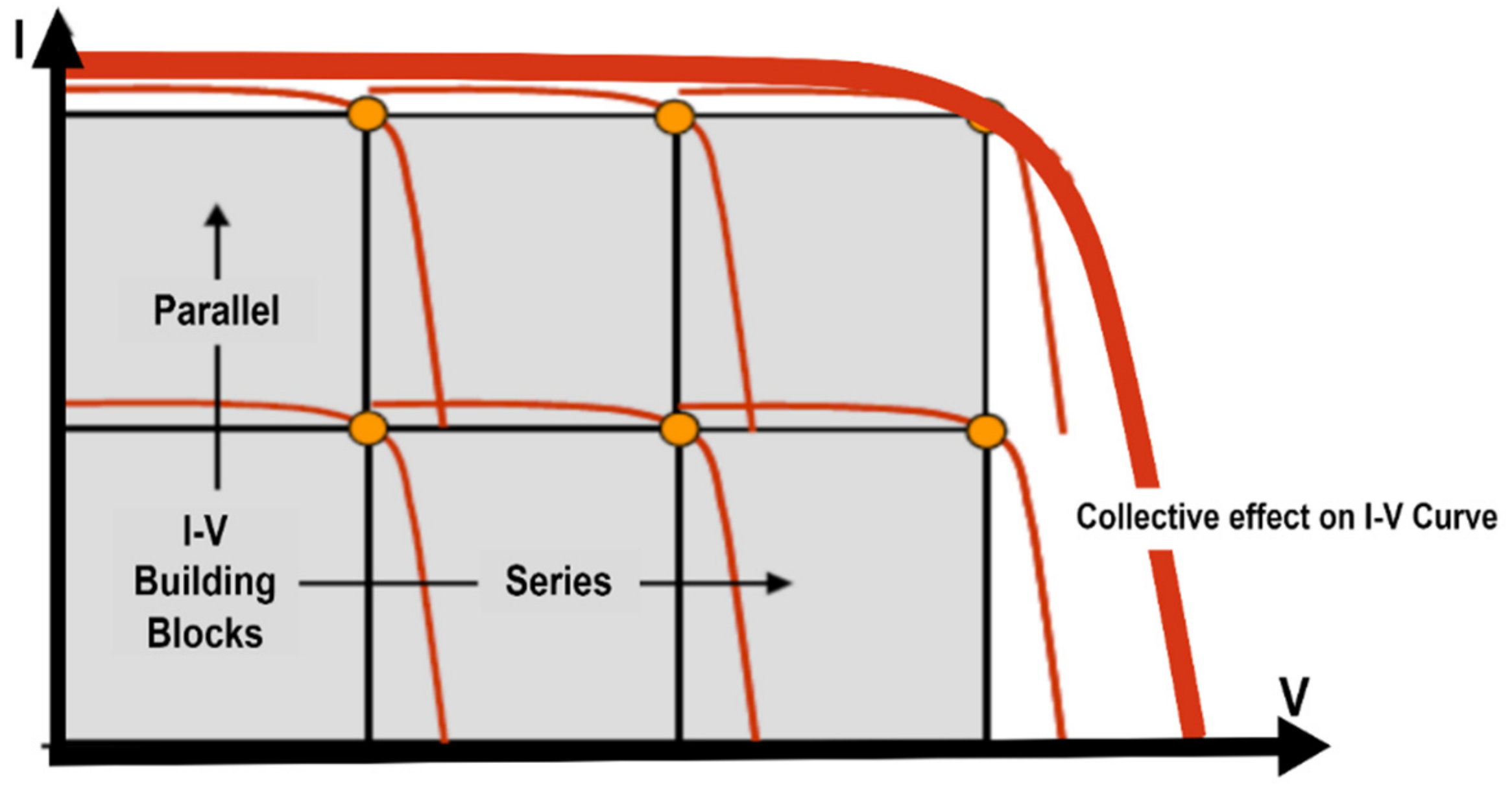
The I-V curve of each module of PV array maintains its form, however it scales related to the number of cells are linked in series and parallel. Figure 2 is obtained by connecting n and m cells in series and parallel [28]. The parasitic elements, i.e., series resistance (R_s) and shunt resistance (R_sh), in the model have a substantial impact on a PV module’s performance. When modeling the behavior of PV modules, it is crucial to have a thorough grasp of the series and shunt resistances. The solar cell efficiency is diminished during operation owing to power loss through internal resistances. 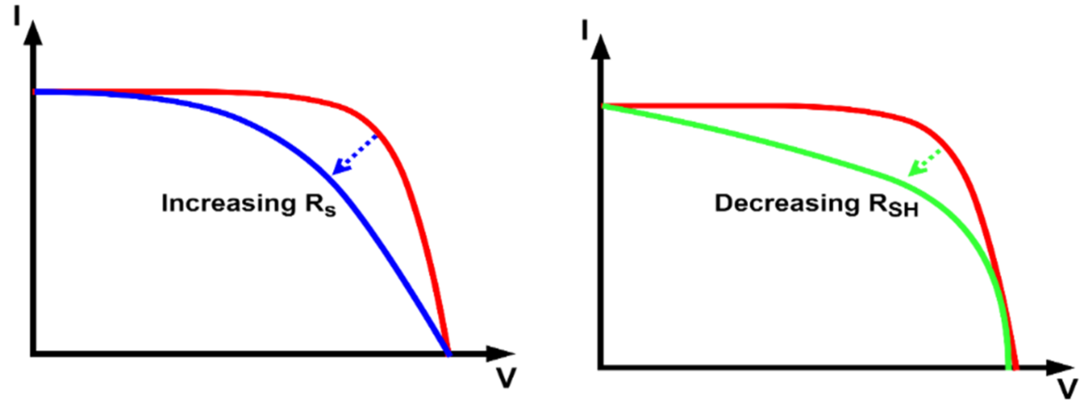Figure 3 shows the effect of parasitic resistances on the PV characteristics.

In an ideal cell, R_sh is infinite because there lies no other route for current to travel, and R_S is zero since there is no more voltage drop at the load. When R_sh is reduced and R_s increased, the fill-factor and maximum power are reduced. When R_sh is lowered too much the open circuit voltage (V_OC) will drop, whereas when R_S is increased too much, a short circuit current (I_SC) will decrease. Changes in irradiance have a huge impact on a PV system’s current and power output, but they have a much smaller impact on the voltage. PV systems are ideal for battery charging because the voltage varies only a little with the amount of sunlight [28].

The non-linear P-V curves of PV system become increasingly complicated involving many peaks [29] under partial shading conditions, which is one of the main reason for power loss in PV systems. In order to protect PV modules from flashing, or in other words preventing a hot spot problem, by-pass diodes are connected in parallel to each PV module. A combination of series connected modules make up a string of modules. Several such strings are connected in parallel in a PV array. Due to partial shading, there is a potential difference between these strings. In order to prevent the flow of current from one string to another, blocking diodes are used at the start of each string. As a result of the bypass diodes and under partial shading conditions, several local MPPs may exist in the P-V characteristic of the PV array, whereas a single MPP may exist under constant insolation. Figure 4 depicts a PV array made up of 6 modules under PSC.

The MPP of PV system, which is of a maximum power at a defined operating point, is aggressively sought by an MPPT controller. An MPPT controller is a system which calculates the voltage or current at which a PV system should produce maximum power under changing atmospheric conditions. It controls the output of PV modules so that they may create the maximum amount of power possible [30]. A suitable DC–DC converter, along with a suitable tracking algorithm, constitutes an effective MPPT controller with several desirable characteristics. These including being budget-friendly, simple to implement, containing a quick tracking response for dynamic analysis, an ability to track the maximum power point throughout a wide-range of solar radiation and temperature levels, and without any oscillation around the maximum power point. Under chilly, cloudy, or foggy weather, an MPPT controller is most effective for charging a discharged battery as the controller can deliver more current for charging.

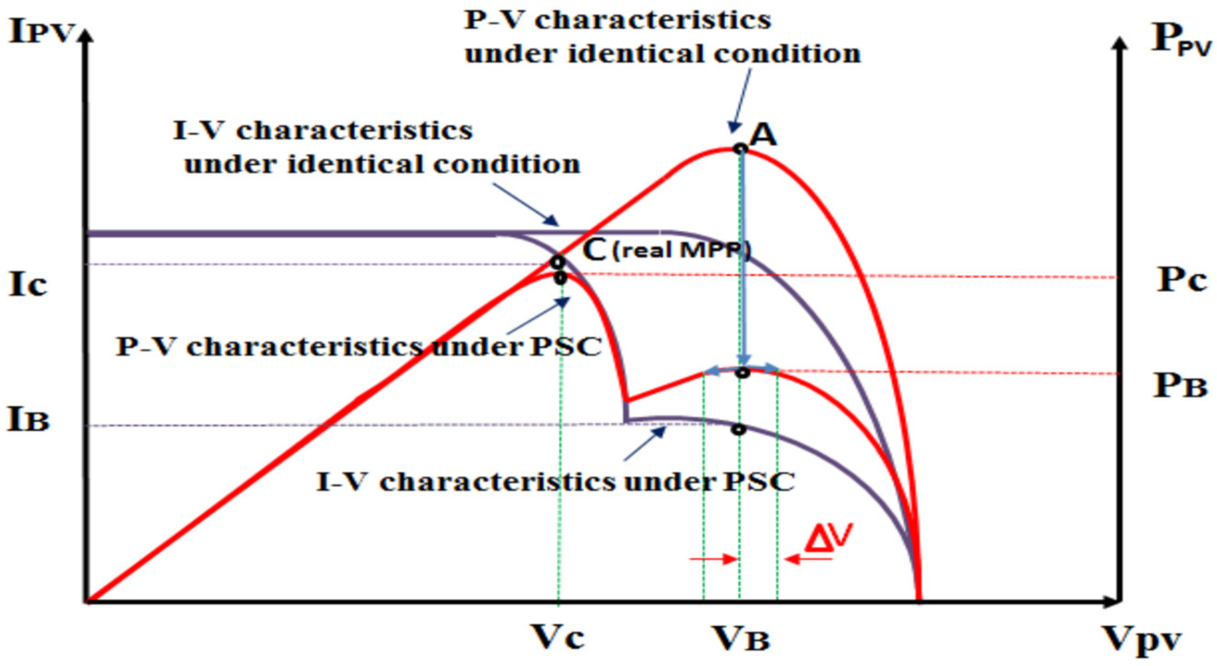
The effectiveness of conventional MPPT methods, such as incremental conductance, P&O, and hill climbing, decreases under partial shading conditions due to multiple local maxima in the PV characteristics; however, their competence is reported to have been greater than 99 percent under constant insolation.

The cause of MPPT failure under PSC is depicted in Figure 5. Point “A” is the location of the operating point prior to PSC. The operating point is then moved to point “B” after PSC, whereas the true MPP is at point “C” in Figure 5. Conventional techniques cause the operating point to fluctuate near point “B” due to a predefined voltage reference step. At the same time, the difference in power capacity between the P_C and the P_B is lost owing to the MPPT failure. MPPT techniques must change the operating point to “point C” to avoid power loss [31].

2.1. DC–DC Converter

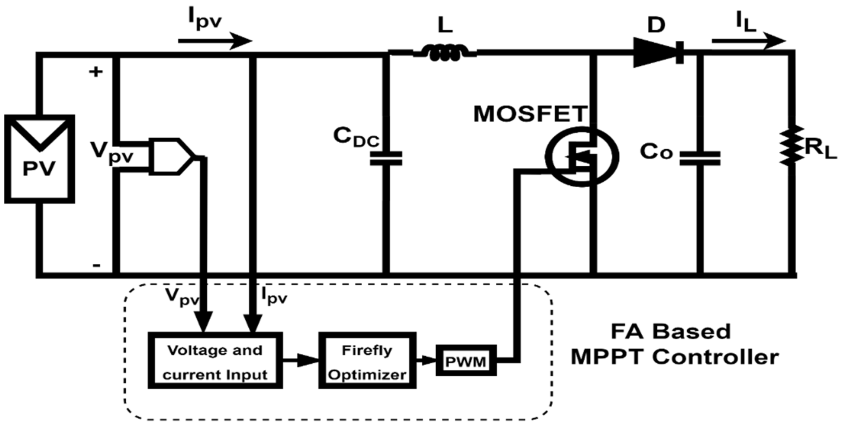
A DC–DC converter changes magnitude of input voltage to variable DC output voltage, normally an unregulated DC to regulated DC. An inductor, capacitors, and switches comprise a DC–DC convertor. These converters perform duties like as charge controllers, maximum power point trackers, and PV load interfaces as shown in Figure 6. A buck and boost DC–DC converter is most commonly used in literature due to its simple construction and low component count [32].

A buck converter is a kind of step-down converter and produces a smaller output from its larger input voltage. A boost converter is also known as a step-up converter. A boost convertor is an electrical device that converts a lower input voltage into a higher output value. A converter comprises of a MOSFET as a switch, diode, inductor, and a capacitor. Its output voltage is related to the input voltage through the following relationship, where D is the duty cycle [32].

$$V_{in}=\left(1-D\right)V_{out}$$

(7)

2.2. System Description

The proposed Firefly Algorithm-based MPPT system is illustrated as a block diagram in Figure 7. Its structure is made up of four PV modules that are linked in series. Temperature, irradiance, and partial shading circumstances all have an impact on the PV module’s performance. An MPPT controller is required for the PV array to run at its maximum output (MPP). The Firefly Algorithm (FA) based MPPT controller is used with a DC–DC boost converter. Due to the PV cell production efficiency, which currently does not exceed 15%, the Firefly Algorithm will track MPP more quickly and efficiently.

The PV array must be selected as per maximum sanction load. A Tata Power Solar Systems TP250.MBZ has been used as a test setup. This module also comprises 60 cells in series having a maximum output of 249 watts. The maximum power of the array is determined using Equation (8). Since N_p and N_s denote parallel and series modules, respectively, I_mp denotes total PV module current at the MPP and V_mp denotes total PV module voltage at MPP.

Using standard testing conditions (STC):

$$P_{mp}=(N_P\times I_{mp})\times (N_s\times V_{mp})=\left(1\times 8.3\right)\times \left(4\times 30\right)=996.2$$

(8)

The photovoltaic specifications of the single module are described in

Table 1. Specifications of solar module.

Parameter	Value	Unit
Open circuit voltage (Voc)	36.8	V
Shot circuit current (Isc)	8.8	A
Voltage at MPP (Vmp)	30	V
Current at MPP (Imp)	8.3	A
Max. power	249	W
Number of series modules (Ns)	4	-
Number of parallel modules (Np)	1	-

. Figure 8, Figure 9 and Figure 10 show the impact of irradiance on photovoltaic characteristic curves.

In Figure 8, the P-V curves of the solar module can be seen at different irradiances i.e., 1000 W/m², 900 W/m², 800 W/m^2, and 500 W/m² at constant temperature of 25 °C.

In Figure 9, the V-I curves of solar module can be seen at different irradiances and at a constant temperature.

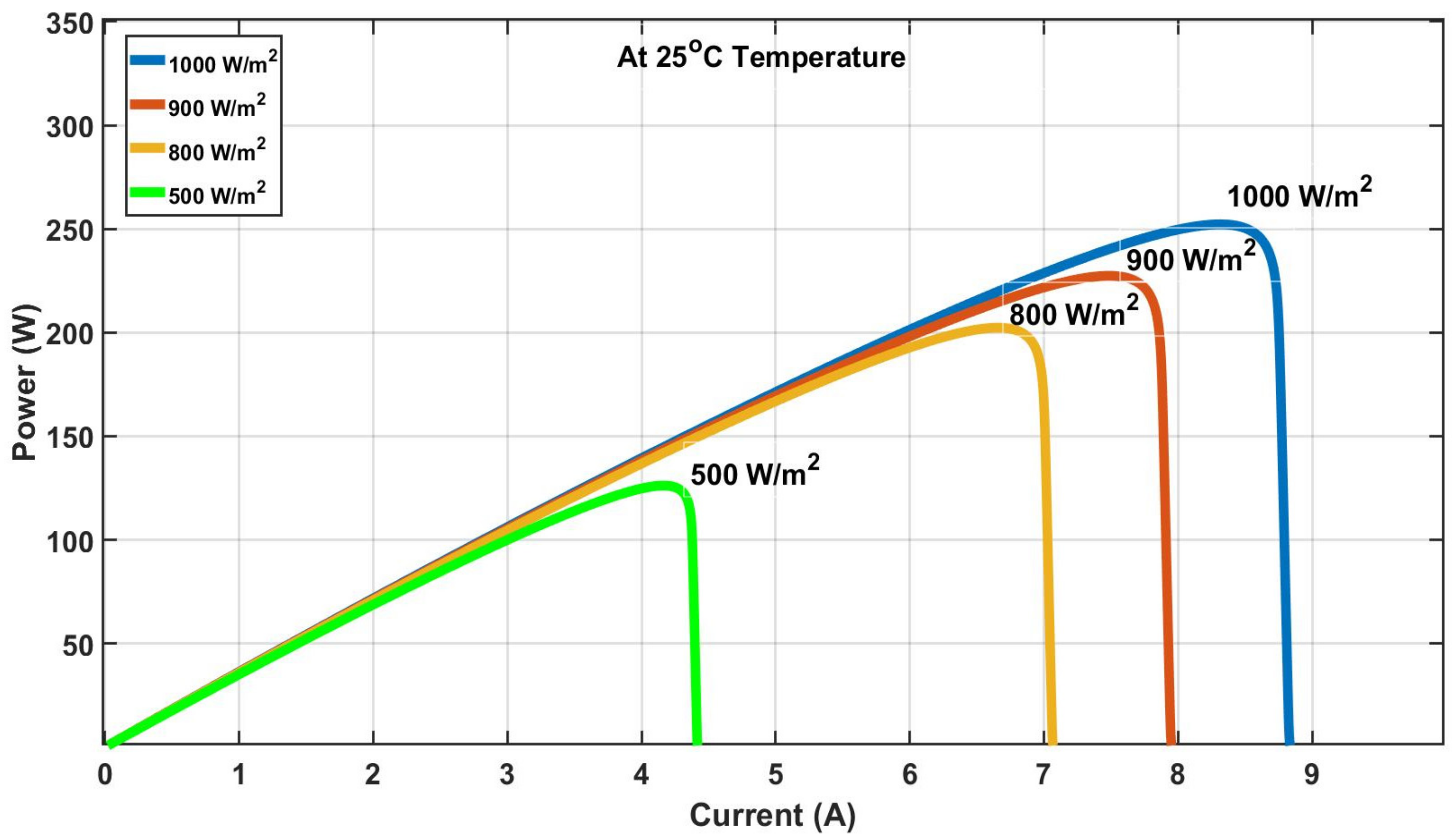
In Figure 10, it is clear that the current varies significantly with irradiance. The P-I curves of a solar module can be seen at different irradiances and at a constant temperature. Similarly following three figures, Figure 11, Figure 12 and Figure 13 show the impact of temperature variation on the photovoltaic characteristics.

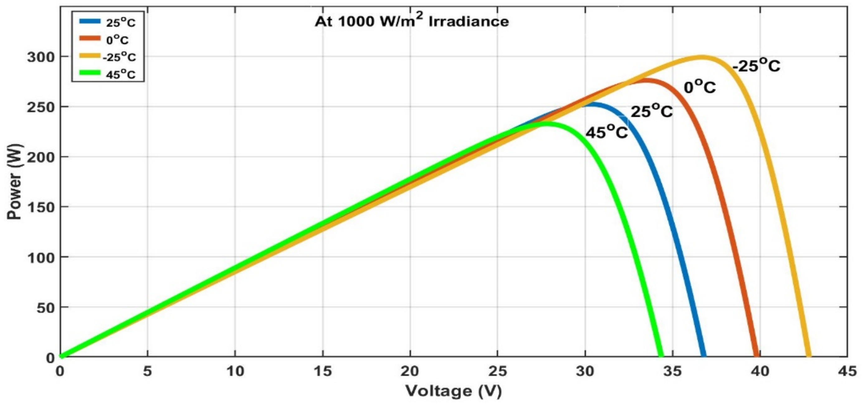
As can be seen, the MPP has changed and due to temperature variation, the open circuit voltage (V_oc) is greatly affected. In Figure 11, the P-V curves of the solar module are shown at different temperatures i.e., −25 °C, 0 °C, 25 °C, and 45 °C at constant irradiance of 1000 W/m².

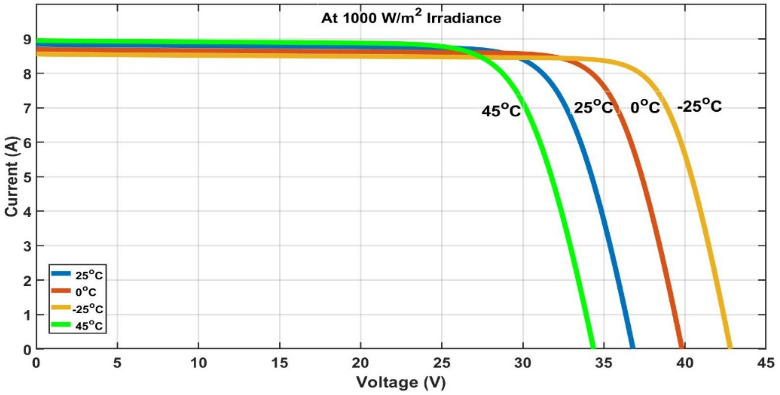
Whereas in Figure 12, it can be seen that V_oc varies significantly with the temperature, the I-V curves of the solar module can be seen at different temperatures and at a constant irradiance. In Figure 13, the P-I curves of the solar module are shown at different temperatures and at a constant irradiance.

Because partial shading causes several peaks, most MPPT algorithms cannot work appropriately and converge to a local MPP under these conditions. This paper presents a Firefly Algorithm-based optimization technique for the tracking of the maximum power point, which solves the problem caused by the partial shading condition.

There are capacitors that are often built to accommodate energy needs during switching moments, which are equivalent to fast changes in irradiation and load. Equation (9) is used to design a DC-link capacitor that is used with the PV array, as shown in Figure 7.

$$P_{mp}\times \Delta t=\frac{1}{2}{C}_{dc}\left[V_{dc}^2-V_{min}^2\right]$$

(9)

where V_dc denotes the DC-link or PV voltage, V_min denotes the minimum PV permitted voltage, and Δt is the flash duration. The system’s switching frequency (f_s) is 50 kHz. When V_dc is equal to the PV array voltage at MPP (120 V), V_min is half of the photovoltaic array voltage at maximum power, i.e., 60 V, the value of Δt is three times the switching period, and C_dc is around 10 µF.

The output voltage V_o is controlled at a set value by DC–DC boost convertors. This value is supposed to be double the PV array voltage at MPP for design purposes (240 V). During a drop in irradiance or significant partial shade, the output filter capacitor (C_o) delivers load energy. As a result, a time of 1-ms has taken hold. Using the same basic equation as before, but with a V_min of 120 V and P_mp of 996 W, the value of C_o should be at least 0.23 mF.

Without accounting for PV and boost converter losses, the output power capacity is equal to input power (996 W), resulting in an equivalent load resistance of around 58 Ω, as shown in the equation below.

$$R_L=\frac{V_o^2}{P_{mp}}=\frac{{240}^2}{996}=58\Omega$$

(10)

Minimum and maximum duty cycle are established, as shown in the formulae below, to build the boost converter inductance.

$$D_{min}=\frac{V_o-V_{dc,max}}{V_o}=\frac{240-120}{240}=0.5$$

(11)

$$D_{max}=\frac{V_o-V_{dc,min}}{V_o}=\frac{240-60}{240}=0.75$$

(12)

The minimum duty cycle and V_dc,max are used to ensure the photovoltaic array current in continuous conduction mode. As a result, the inductance value is:

$$L=\frac{V_{mp}\times D_{min}}{\Delta I_{dc}\times f_s}=\frac{120\times 0.5}{1\times 50\times {10}^3}=1.2 \mathrm{mH}$$

(13)

2.3. Firefly Algorithm Based MPPT Controller

As was discussed in Section 1, the FA is a swarm intelligence-based metaheuristic algorithm. As the distance between fireflies increases, the intensity of light decreases as per the inverse square law, i.e., $I\left(r\right)=\frac{I_s}{r^2}$. In addition, the air also absorbs the light which becomes weaker with the distance. To improve the convergence to the global optimum, the selection of suitable parameter values is crucial. Inappropriate choices might result in computational inefficiency. The attractiveness parameter is another variable. The firefly is attracted and tends to move towards to a brighter firefly j according to Equation (15). The attractiveness $\beta$ can be quantitatively stated as in Equation (14) [33].

$$\beta \left(r\right)={\beta }_o{e}^{-\gamma r^m}, m\ge 1$$

(14)

Equation (15) determines distance between the two fireflies i and j at position x_i and x_j, respectively.

$$r_{ij}=\left|\right|x_i-x_j\left|\right|$$

(15)

$$x_i=x_i+{\beta }_o{e}^{-\gamma r_{ij}^2}\left(x_i-x_j\right)+\alpha {\epsilon }_i$$

(16)

${\beta }_o$ represents initial attractiveness at r = 0 in Equations (14) and (16). r represents the distance between two fireflies. $\gamma$ represents the absorption coefficient that controls the reduction of intensity of light. Its value determines the behavior of the FA algorithm and is crucial in determining the speed of convergence [23]. Where m is an integer and is set to 2, $\alpha$ is the randomization term, with ${\epsilon }_i$ being a random number generator uniformly or normally distributed in [0,1].

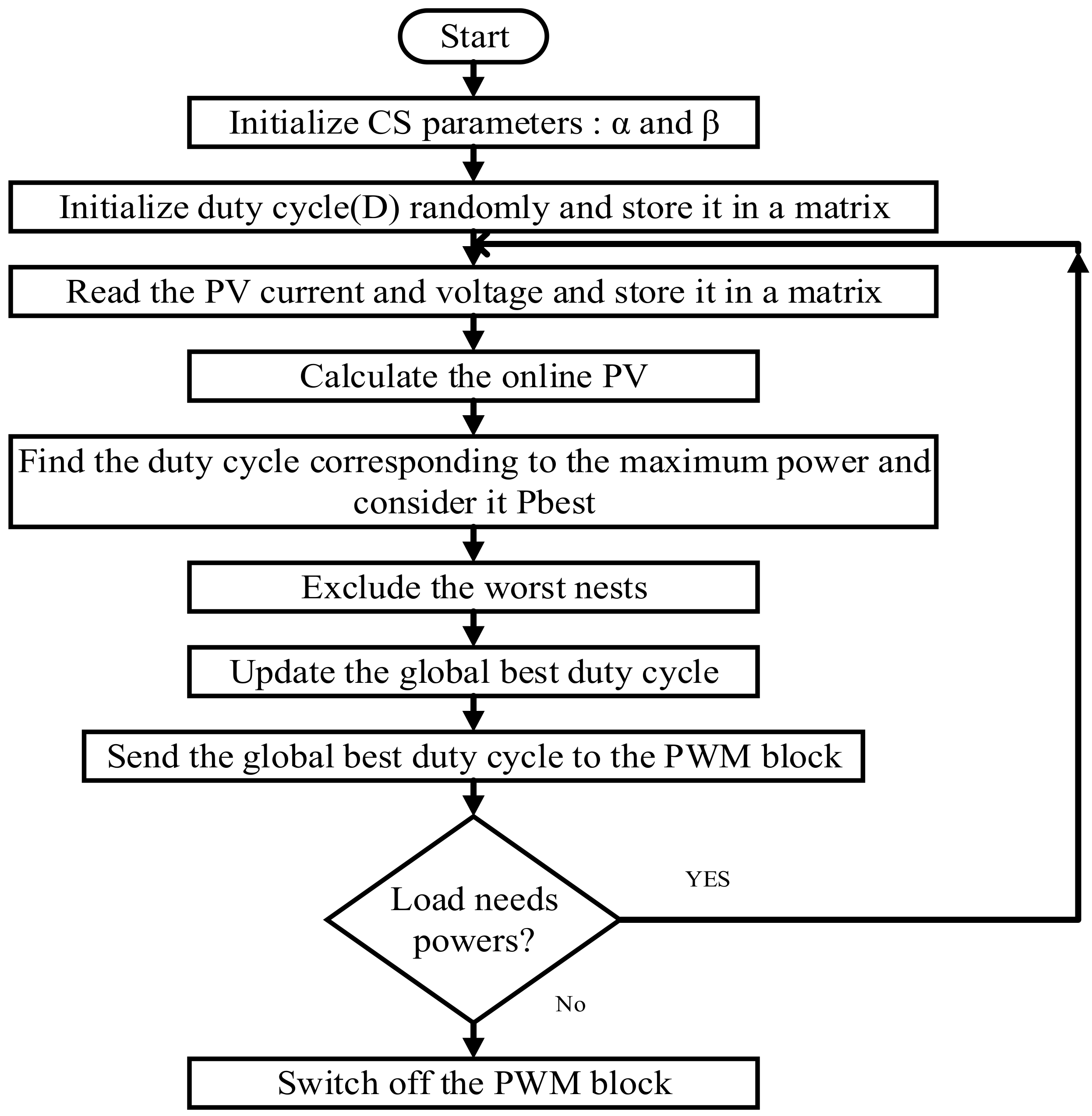
While implementing the algorithm for MPPT, the PV voltage is selected as the regulated variable and the objective function is taken as the PV power. Figure 14 shows the flowchart of the FA-based MPPT controller.

Table 2. Terminology of FA vs PV system.

Firefly Algorithm for Optimization	PV System
Firefly position $(x_i)$	Reference Voltage (Vref)
Distance $(r_{ij})$	Voltage difference (ΔVref)
Attractiveness $({\beta }_o$)	Exponential function of ΔVref
Brightness	Power (Ppv)
Brightest Firefly	Global maximum power (PGbest)

shows terminology of FA versus PV system as given below.

The following are the steps of achieving MPPT using an FA algorithm.

• Set the starting parameters of the Firefly Algorithm, i.e., the attractiveness and randomization.
• Initialize the magnitude of the population i.e., the number of PV modules.
• Simulate the Simulink model.
• Obtain the output power that corresponds to the firefly’s brightness.
• Depending on the optimization strategy used, update the duty cycle value indicated by the location of the firefly.
• Examine the constraints and implement the best solution.

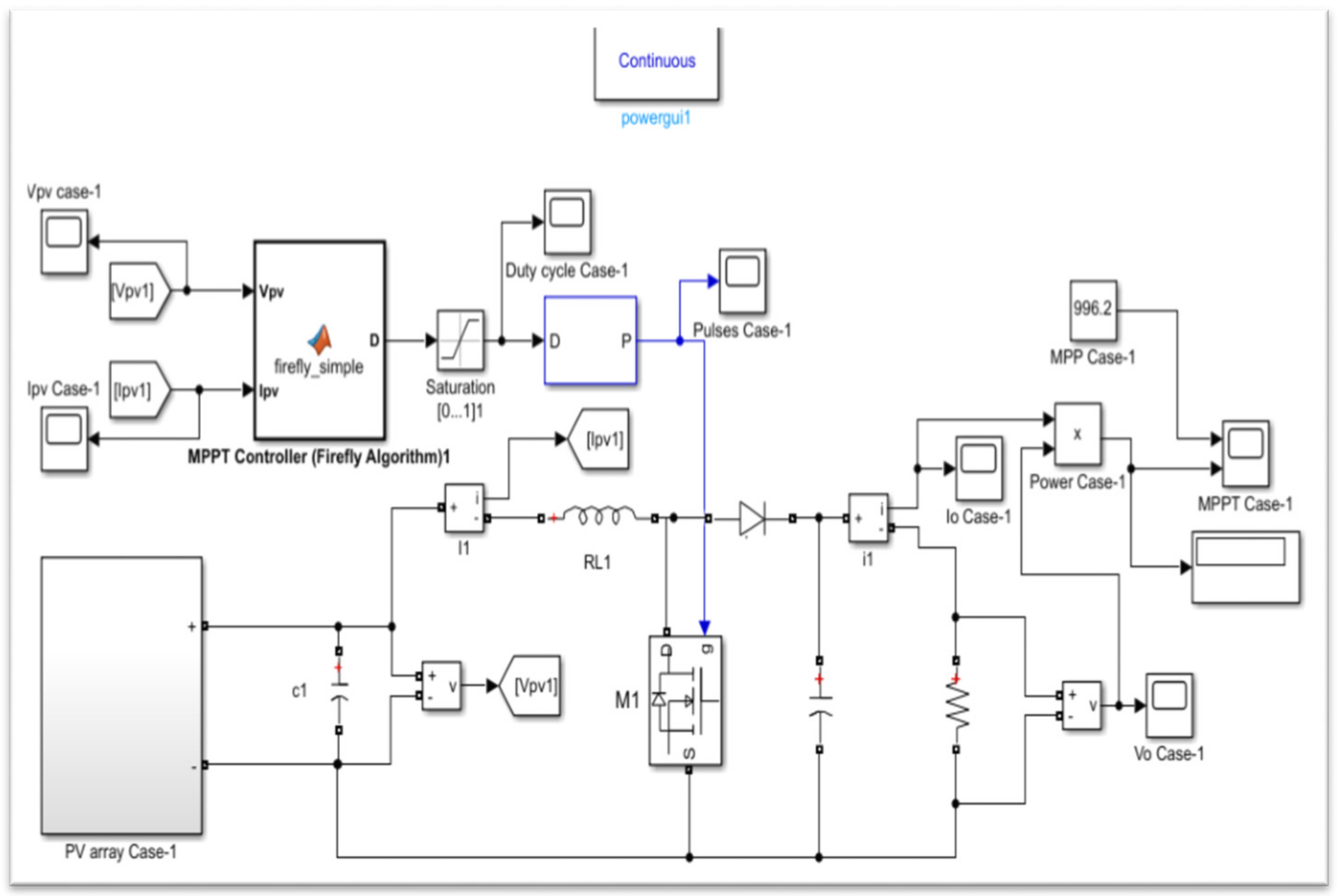
The model and algorithm were tested using Matlab/Simulink. Figure 15 shows the modeling of the PV array in Simulink. The testbed setup includes a PV Array, an FA-based MPPT controller, a boost converter, and a load, as shown in Figure 16.

3. Results

This section compares the results of FA, PSO, PID, and P&O-based MPPT controllers. Different test cases are introduced in this section, which considered all possible operating situations, including normal and shading scenarios. It also includes a comprehensive comparative analysis of the Firefly Algorithm technique and conventional methodologies.

The accuracy and performance of recommended techniques are tested using a PV system. During this simulation, four Tata Power Solar Systems TP250MBZ PV panels, a DC–DC boost converter, and an MPP control system were used. In order to compare the performance of the Firefly optimization method with the PSO, P&O, and PID schemes, five examples were simulated and examined.

Table 3. Irradiance and temperature profile of all Cases.

PV Modules	PV Module 1		PV Module 2		PV Module 3		PV Module 4		GMPP (W)
Inputs	Ir (W/m2)	Temp (°C)	Ir (W/m2)	Temp (°C)	Ir (W/m2)	Temp (°C)	Ir (W/m2)	Temp (°C)
Case 1	1000	25	1000	25	1000	25	1000	25	996.2
Case 2	300	25	900	25	300	25	900	25	438.94
Case 3	300	45	900	45	300	45	900	45	403.7
Case 4	800	25	1000	25	500	25	1000	25	637.7

shows the irradiance and temperature profile for all cases.

• Case 1: Normal operation at STC (Uniform Irradiance and Temperature).
• Case 2: Partial shaded conditions with two Peaks at STC temperature.
• Case 3: Partial shaded conditions with two peaks at non-STC temperature.
• Case 4: Partial shaded conditions with three peaks at STC temperature.
• Case 5: Varying irradiance and Varying temperature.

In Figure 17 and Figure 18, photovoltaic array P-V and I-V curves under all situations are shown.

3.1. Normal Operation at STC/Uniform Conditions (Case 1)

In this condition, irradiance is 1000 W/m² at 25 °C for all modules in the PV array. Figure 19 and Figure 20 show the P-V, I-V curves of the array under normal operation at standard testing conditions (STC), respectively. Figure 21 shows the tracking of MPP using the FA algorithm, whereas Figure 22 and Figure 23 show the V_pv and duty cycle plots, respectively.

The comparison between the Firefly Algorithm and traditional methods of MPPT, along with MPPT curves for the FA, PSO, PID, and P&O algorithms, are shown in Figure 24. It is clear that the suggested FA MPPT controller has a higher accuracy and better time response. Figure 19 shows that there is one peak in the P-V curve at 996.2 W, 122.2 V. This is the maximum power point in case-1, achieved by a MPPT controller. This indicates that there are no local peaks. In Figure 20, the I-V characteristics show that the current at MPP is 8.14A.

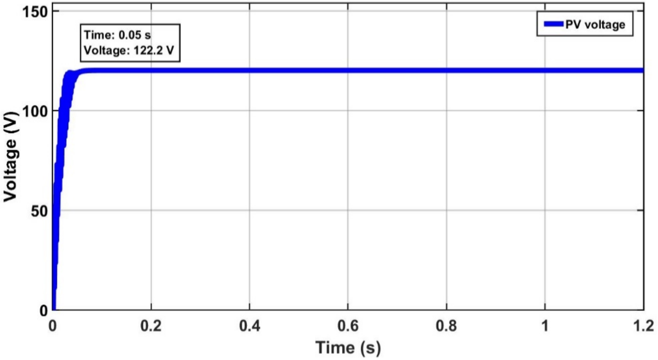
In Figure 21, it is clear that FA technique for MPPT is achieving the maximum power of 996.2 in 0.05 sec under case-1 conditions, which is very fast and effective. Moreover, it keeps on tracking the MPP until the end of the simulations. The result shows that this algorithm is controlling the MPP in a very smooth manner without any fluctuations or delay time. Figure 22 shows the V_pv monitoring throughout the simulation in case-1, which shows that the voltage at the MPP is 122.2V. During the charging of capacitors and the inductor’s inrush current, the voltage fluctuates initially but becomes stable in a minimum time of 0.05 s. 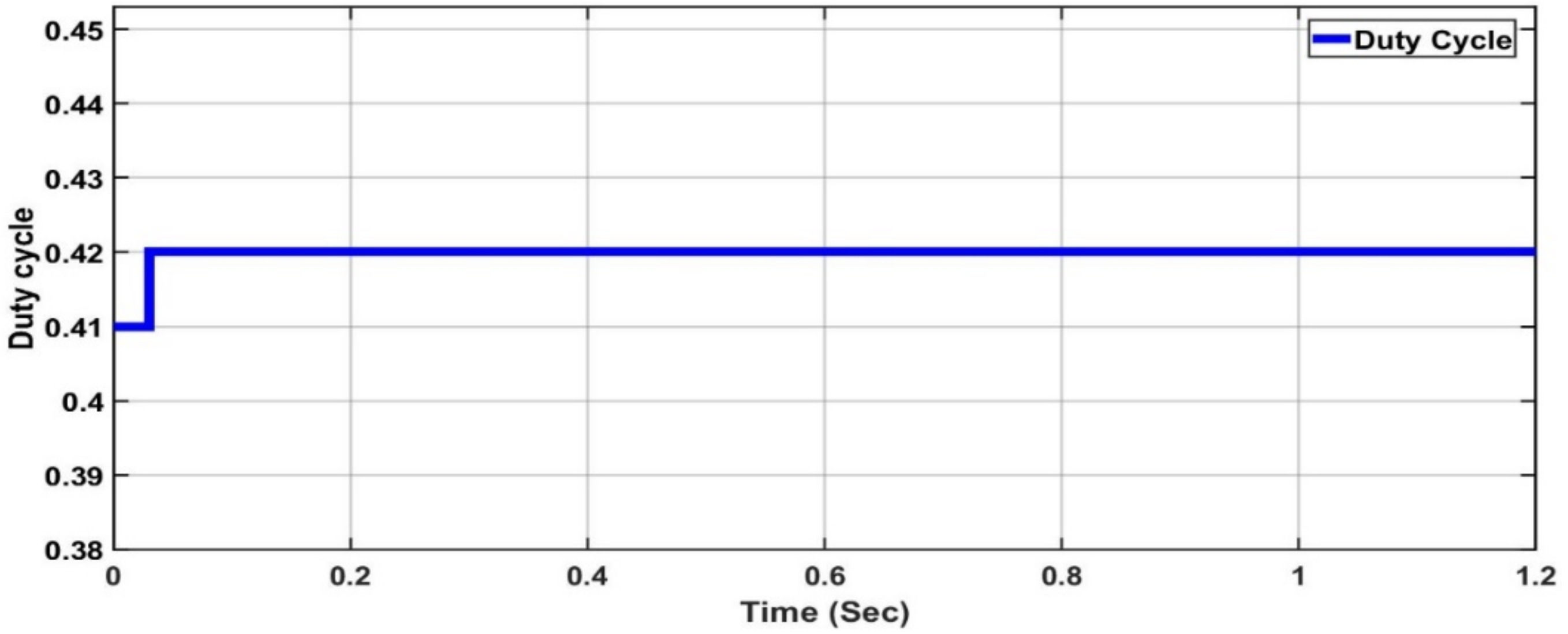After 0.05 s, both the voltage and power become normalized and smooth, i.e., without fluctuations, whereas Figure 23 depicts the duty cycle obtained from the MPPT controller in case-1 using the FA algorithm.

In Figure 24, it is clear that the FA technique is much better than the old PSO algorithm and conventional PID and P&O methods. The results clearly indicate that the suggested FA achieves an MPP of 996.2 W, whereas PSO, PID, and P&O failed to achieve the peak points, even within uniform conditions. Further analysis shows that the PSO for tracking the MPP outperforms the PID and P&O methods as the MPP obtained from the PSO, PID, and P&O methods is not smooth. The proposed FA algorithm achieves the maximum power point in a minimum time of 0.05 s, whereas PSO, PID, and P&O techniques are comparatively slower. A fluctuation can be seen in the PSO MPPT graph at a time of 0.37 s. After that time it becomes stable at its maximum power point of just 910 W. Whereas P&O achieved a MPP at 720 W, in comparison with these three techniques, the FA algorithm achieved the MPP at 996.2 W, i.e., the maximum result that can be achieved under case-1 conditions, as per the P-V and I-V curves of the array.

3.2. PSC with Two Peaks & STC Temperature (Case 2)

During this condition, irradiances of PV Module 1, 2, 3, and 4 of PV array are 300 W/m², 900 W/m², 300 W/m², and 900 W/m², respectively. The temperature for all the four PV modules is constant at 25 °C. Figure 25 and Figure 26 show the P-V and I-V curves of the solar array in case-2 conditions. Figure 27 shows the tracking of MPP using an FA algorithm under case-2 conditions, whereas Figure 28 and Figure 29 show the V_pv and duty cycle plots, respectively. To compare the FA with the older methods of the MPPT, the MPPT curves for the FA, PSO, PID, and P&O algorithms are shown in Figure 30. Results show that the FA–MPPT controller is more accurate and has a better time response compared to other three techniques under case-2 conditions (i.e., partially shaded conditions with one local and one global peak).

In Figure 25, one can see that there are two peaks of the PV curve at 438.9 W, 59.81 V and 326.29 W, 130.46 V, which are called the global peak and local peak, respectively. As such, the global peak is at 438.9 W, which is the maximum power point that has to be achieved by an MPPT controller in case-2. In Figure 26, the I-V characteristics show that the current at the MPP is 7.33A. In Figure 27, the FA technique for the MPPT achieved the maximum power of 438 W in 0.05 s under case-2 conditions, which is very fast and effective. It continues stably tracking the MPP until the end of the simulation. The result shows that without any fluctuations and delay time, this algorithm is controlling the MPP under partially shaded conditions (case-2) in a very smooth manner. Figure 28 shows the V_pv monitoring throughout the simulation in case-2, which shows that the voltage at MPP is 59.81 V. It can be seen that voltage gets stable and achieved its maximum value in a minimum time of 0.05 s. After 0.05 s, the voltage and power are both smooth, i.e., without fluctuations. Figure 29 depicts the duty cycle obtained from the MPPT controller in case-2 using the FA algorithm under partially shaded conditions.

From Figure 30, it can be seen that the FA technique is much more efficient than the old PSO, PID, and P&O methods. The results clearly depict that the FA achieved an MPP of 438 W, whereas the PSO, PID, and P&O methods failed to achieve the maximum point in partially shaded conditions. This comparison represents the effectiveness of the suggested FA algorithm. Further analysis shows that the PSO for tracking the MPP outperforms the PID and P&O methods. Moreover, the FA algorithm technique is smooth and without fluctuations in power, whereas the MPP achieved from the PSO, PID, and P&O methods were not smooth. Fluctuations can be seen in their MPPT graphs. Also, the FA algorithm achieved the maximum power point in a minimum time of 0.05 s, whereas the PSO, PID, and P&O techniques were slower than with the proposed algorithm. A fluctuation can be seen in the PSO and PID MPPT graph throughout the simulation because it is trying to achieve a global peak while trapped between the global peak and local peak. In comparison, the P&O achieved an MPP of only 315 W. In comparison with these three techniques, the FA algorithm achieved the MPP of 438 W, as the maximum power that can be achieved under case-2 is 438.9 as per P-V, I-V curves at the PSC of case-2.

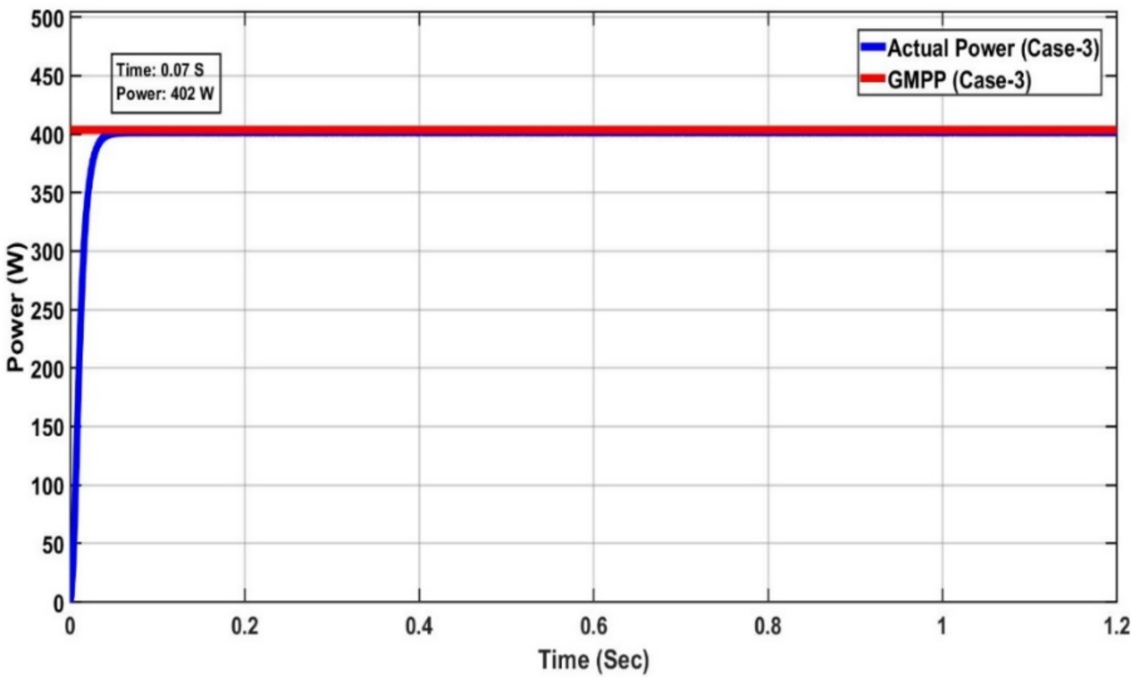
3.3. PSC with Two Peaks at NON-STC Temperature (Case-3)

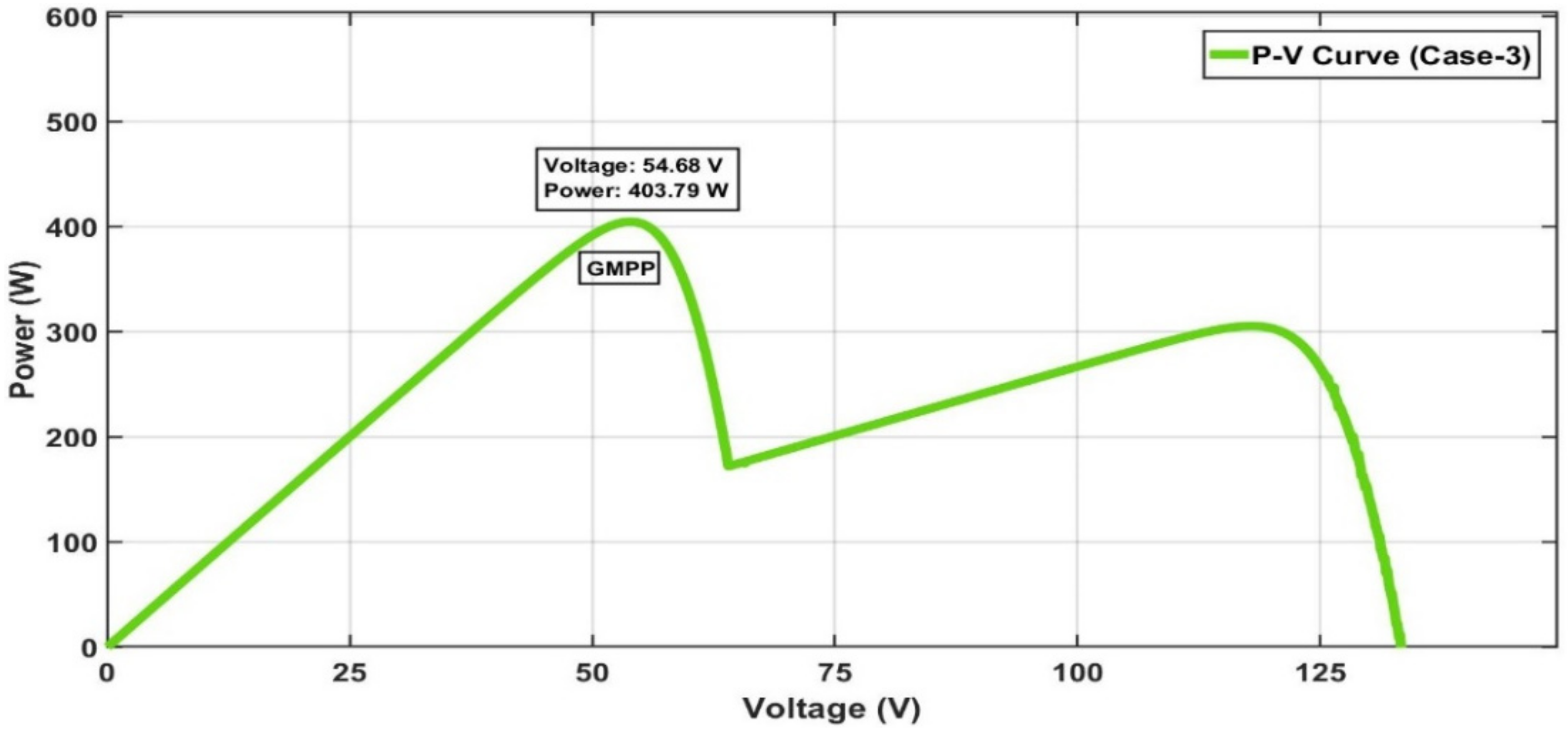
In this condition, irradiances of PV Modules 1, 2, 3, and 4 of the PV array are 300 W/m², 900 W/m², 300 W/m², and 900 W/m², respectively. The temperature for all the four PV modules in this case is 45 °C, more than the STC temperature (25 °C). Figure 31 and Figure 32 show the P-V, I-V curves of solar array at the PSC (Case-3). Figure 33 indicates the tracking of MPP using the FA algorithm under case-3 conditions, whereas Figure 34 and Figure 35 show the V_pv and duty cycle plots respectively under case-3 conditions. For a comparison of the FA technique with the other old techniques of MPPT, MPPT curves for the FA, PSO, PID, and P&O algorithms are shown in Figure 36. The results conclude that the FA–MPPT controller is more accurate and has a better time response compared to other three techniques under case-3 conditions (i.e., partially shaded conditions with one local and one global peak at a NON–STC temperature).

Figure 31 shows that there are two peaks of the PV curve at 403.7 W, 54.68 V and 310 W, 120 V, which are referred to as the global peak and local peak, respectively. As such, the global peak is at 403.7 W, and it is the maximum power point that has to be achieved by an MPPT controller in case-3. In Figure 32, the I-V characteristics show that the current at MPP is 7.38A, whereas the voltage at MPP is 54.68 V.

In Figure 36, it can be seen that the FA technique for MPPT achieved the maximum power of 402 W in 0.07 s under case-3 conditions, which is very fast and effective. It continues stably tracking the MPP until the end of simulation. This result shows that this algorithm is controlling the MPP under partially shaded conditions and a NON–STC temperature (case-3) in a very smooth manner without any fluctuations or delay time. 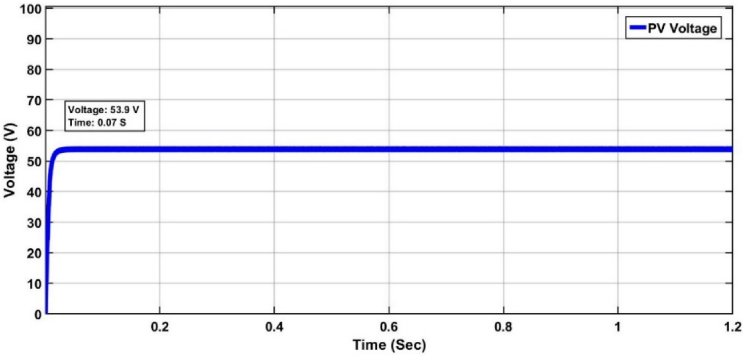Figure 34 shows the V_pv monitoring throughout the simulation in case-3, which shows that the voltage at MPP is 53.9 V. It can be seen that voltage becomes stable at its maximum value in a minimum time of 0.07 s. After 0.07 s, voltage and power both become normalized and smooth, i.e., without fluctuations. Figure 35 depicts the duty cycle obtained from the MPPT controller in case-3 using the FA algorithm under partially shaded conditions and a NON–STC temperature.

From Figure 36, it can be seen that the FA technique is much efficient than the old PSO and conventional PID and P&O methods. The results clearly indicate that the FA achieved the MPP of 402 W, whereas the PSO, PID, and P&O methods failed to track the peak point at PSC and NON–STC temperatures. This comparison shows the effectiveness of the proposed algorithm. Moreover, the FA algorithm technique is smooth and without fluctuations in power, whereas the MPP achieved from the PSO method is not smooth. Fluctuations can be seen in its MPPT graphs. Also, the proposed FA algorithm achieved the maximum power point in a minimum time of 0.07 s, whereas the PSO, PID, and P&O techniques were slower than our proposed algorithm. A fluctuation can be seen in the PSO–MPPT graph throughout the simulation because it is trying to achieve global peak while trapped between the global peak and local peak, whereas P&O achieved an MPP of only 275 W. In comparison with these three techniques, the FA algorithm achieved the MPP of 402 W, as the maximum power that can be achieved under case-3 is 403.7, as per the P-V, I-V curves in the partially shaded conditions of case-3.

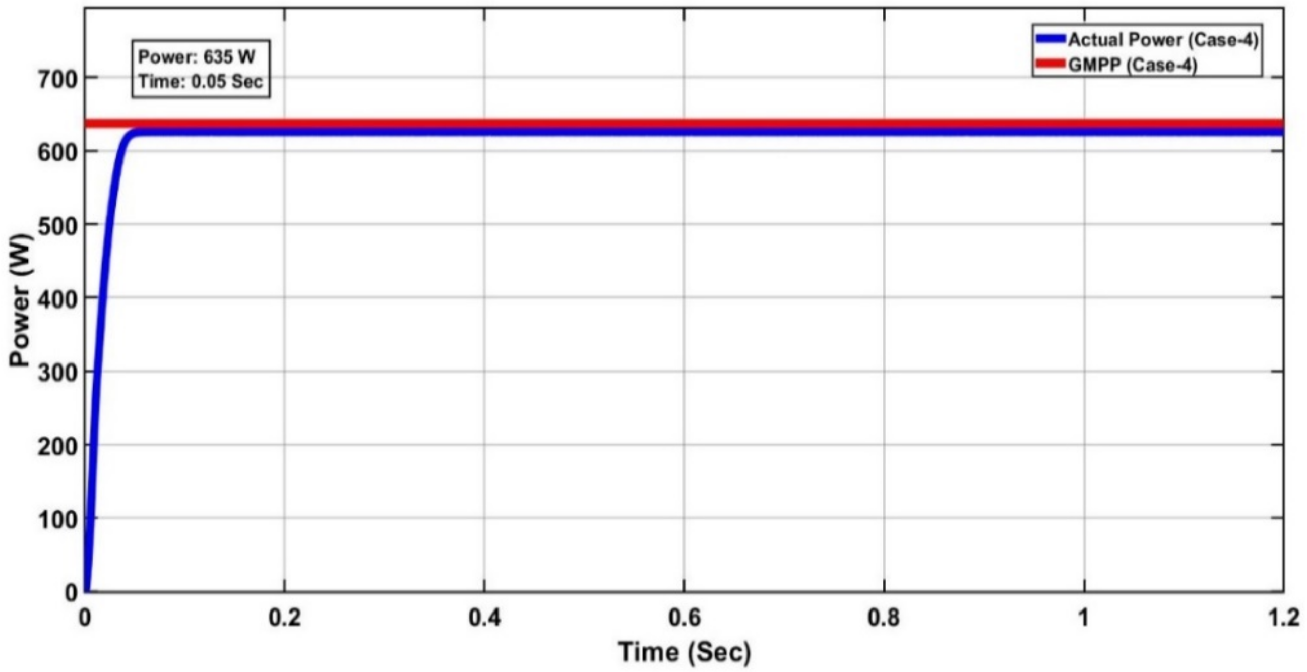
3.4. Partial Shaded Conditions with Three Peaks (Case-4)

In this condition, irradiances of modules 1, 2, 3, and 4 of the PV array are 800 W/m², 1000 W/m², 500 W/m², and 1000 W/m², respectively. The temperature for all the four PV modules in this case temperature is constant at 25 °C. Figure 37 and Figure 38 show the P-V, I-V curves of the solar array under partially shaded conditions with three peaks (Case-4). Figure 39 shows the tracking of the MPP using the FA algorithm under case-4 conditions, whereas Figure 40 and Figure 41 shows the V_pv and duty cycle plots, respectively, under case-4 conditions. To compare the FA method with the other old methods of MPPT, MPPT curves for the FA, PSO, PID, and P&O algorithms are shown in Figure 42. The results conclude that the FA–MPPT controller has a higher accuracy and better time response in comparison with the other three techniques under case-4 conditions (i.e., partially shaded conditions with two local and one global peak).

As in Figure 37, it can be seen that three peaks of the PV curve at 637.7 W, 94.28 V, 486.8 W, 59.5 V and 564.01 W, 132.3 V in which one is GP and the other two are LP respectively. So global peak is at 637.7 W, it is the maximum power point that has to be achieved by a MPPT controller in case-4. In Figure 38, the I-V characteristics show that the current at MPP is 6.76A.

In Figure 39, it can be seen that the FA technique for MPPT achieved the maximum power of 632 W in 0.05 s under case-4 conditions, which is very fast and effective. It continues stably tracking the MPP until the end of simulation. The result shows that this algorithm is controlling the MPP under partially shaded conditions and an STC temperature (case-4) in a very smooth manner without any fluctuations or delay time. 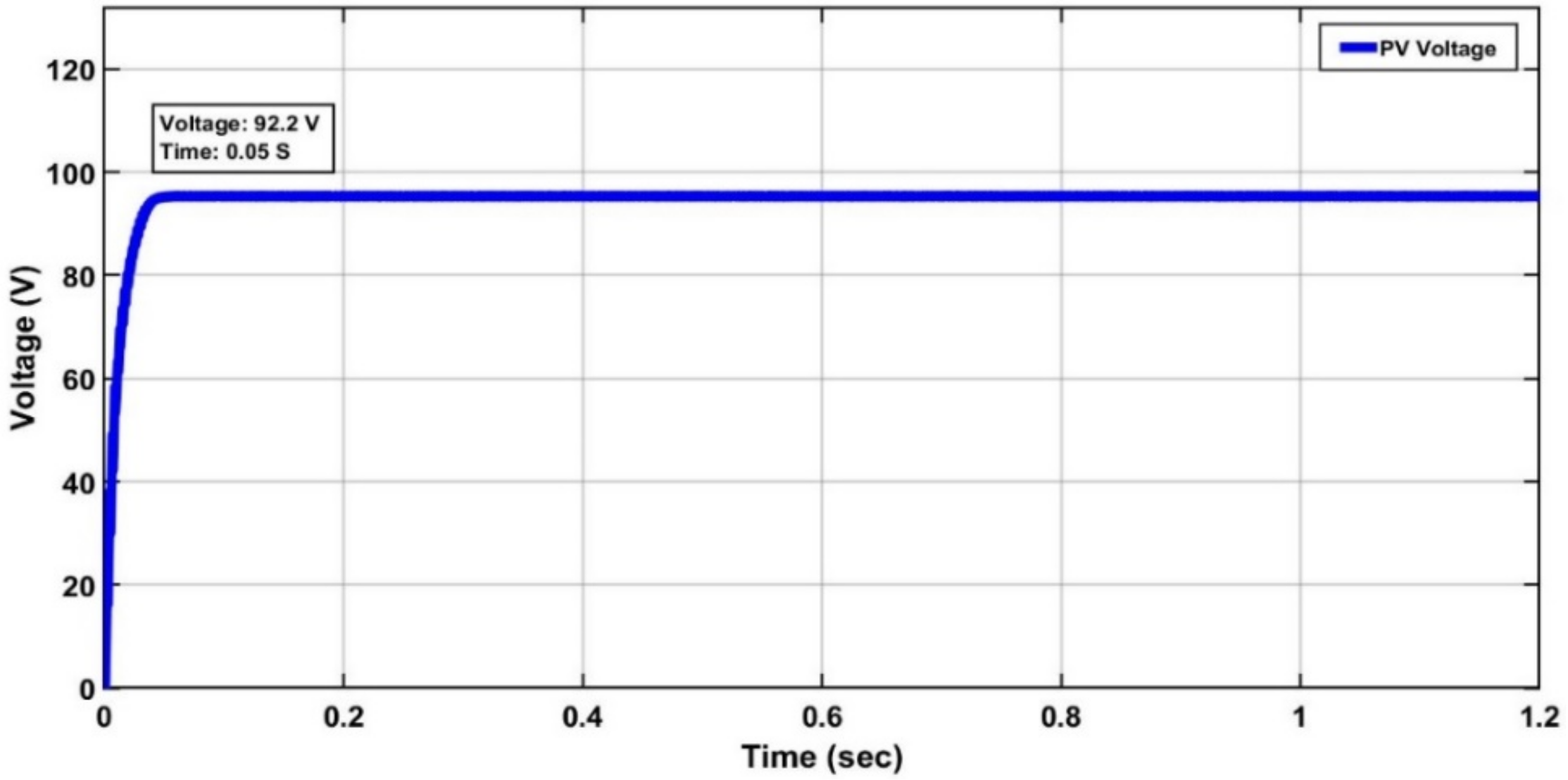Figure 40 shows the V_pv monitoring throughout the simulation in case-4, which shows that the voltage at MPP is 92.2 V. It can be seen that voltage becomes stable and achieves its maximum value in a minimum time of 0.05 s. After 0.05 s, voltage and power both become normalized and smooth, i.e., without fluctuations. Figure 41 depicts the duty cycle obtained from the MPPT controller in case-4 using the FA algorithm under partially shaded conditions and an STC temperature.

From Figure 42 one can see that the FA technique is more efficient than old PSO, PID, and P&O methods. The results clearly indicate that the FA achieved the MPP of 632 W, whereas the PSO, PID, and P&O methods failed to achieve the peak points in partial shading condition with one global peak and two local peaks at the STC. Further analysis shows that the PSO algorithm for tracking the maximum power point is better than the conventional PID or P&O technique. Moreover, the FA algorithm technique is smooth and without fluctuations in power, whereas the MPP achieved from the PSO method is not smooth. Fluctuations can be seen in its MPPT graphs. Also, the FA algorithm achieved the maximum power point in a minimum time of 0.05 s, whereas the PSO and P&O techniques were slower than the proposed algorithm. A fluctuation can be seen in the PSO MPPT graph throughout the simulation because it is trying to achieve a global peak while trapped between the global peak and local peak, whereas the P&O achieved an MPP of only 470 W. In comparison with these three techniques, the FA algorithm achieved the MPP of 632 W, as the maximum power that can be achieved under case-4 is 637.7 W, as per the P-V and I-V curves in partial shading conditions with an STC temperature of case-4.

3.5. Analysis under Varying Irradiance and Varying Temperature (Case 5)

In this scenario, changing irradiance and temperature is fed to the PV array for the analysis of the MPPT controller. For this purpose, 2-signal builder blocks are introduced. One is for irradiance and the second is for temperature. The profile of the signal builder for irradiance and temperature are depicted in Figure 43 and Figure 44.

In this case, temperature and irradiance changes with time. Varying temperature and irradiance profile for PV array is also shown in

Table 4. Varying irradiance and temperature with time.

Time (Sec)	PV Module 1		PV Module 2		PV Module 3		PV Module 4
	Ir (W/m2)	Temp (°C)	Ir (W/m2)	Temp (°C)	Ir (W/m2)	Temp (°C)	Ir (W/m2)	Temp (°C)
0–0.3	1000	25	1000	25	1000	25	1000	25
0.3–0.6	300	25	900	25	300	25	900	25
0.6–0.9	300	45	900	45	300	45	900	45
0.9–1.2	800	25	1000	25	500	25	1000	25

.

From Figure 45, it is clear that the proposed algorithm achieved the MPPT against scenarios of varying irradiance and temperature. Global peaks are also referred in Figure 45 for analysis. The simulation ran for 1.2 s, and 0.3 s were given for each case to run in this simulation and implemented into the system using a signal builder, as shown in Figure 43 and Figure 44.

From Figure 46, one can clearly see that the FA achieved the MPPT with much greater efficiency compared to the PSO and P&O techniques under varying irradiance and temperature cases. An analysis shows that the P&O technique fails under such conditions, whereas the PSO-based technique performs more effectively than the P&O method. The FA achieved the MPPT and remained stable and without fluctuations. When the temperature or irradiance changed, the FA smoothly achieved the MPP with a fast convergence and tracking speed.

The results conclude that the meteorological conditions of temperature and irradiance have a significant impact on power of the PV array. Normal instances with no shading effects, as well as partial shading conditions, were tested. The FA is compared with the PSO, PID, and P&O model to analyze its performance. The results clearly show that the FA algorithm accurately handled all test cases, including partial shading and varying temperature and irradiance cases. The Firefly Algorithm identified the partial shading and tracked the GMPP with smooth and steady behavior without oscillations, having a convergence duration of 0.05 s. On the other hand, conventional algorithms have failed to handle shading conditions. The PSO, PID, and P&O methods exhibited random and unusual behaviors with fluctuations. Furthermore, the conventional algorithms demonstrated unacceptable transient behavior with many oscillations. By utilizing the Firefly Algorithm, the produced energy is maximized and the efficiency is raised.

3.6. Comparison and Analysis with the Other Methodologies

Table 5. Performance comparison of FA, P&O, PID and PSO (Case 1).

MPPT Method	P&O	PID	PSO	FA
Convergence time (s)	0.1	0.1	0.1	0.05
Efficiency (%)	72.2	81.3	91.3	100
Power Oscillations (%)	7	2	1	0
Extracted MPP in [W]	720	810	910	996.2

,

Table 6. Performance comparison of FA, P&O, PID and PSO (Case 2).

MPPT Method	P&O	PID	PSO	FA
Convergence time (s)	0.1	0.1	0.1	0.05
Efficiency (%)	71.7	74	79.7	99.7
Power Oscillations (%)	0	3	3	0
Extracted MPP in [W]	315	325	350	438

,

Table 7. Performance comparison of FA, P&O, PID and PSO (Case 3).

MPPT Method	P&O	PID	PSO	FA
Convergence time (s)	0.1	0.15	0.15	0.07
Efficiency (%)	68.1	71.8	75.5	99.5
Power Oscillations (%)	0	2	3	0
Extracted MPP in [W]	275	290	305	402

,

Table 8. Performance comparison of FA, P&O, PID and PSO (Case 4).

MPPT Method	P&O	PID	PSO	FA
Convergence time (s)	0.1	0.1	0.1	0.05
Efficiency (%)	70.5	78.4	95.6	99.1
Power Oscillations (%)	0	0	4	0
Extracted MPP in [W]	450	500	610	632

and

Table 9. Performance comparison of FA, P&O, PID and PSO (Case 5).

MPPT Method	P&O	PID	PSO	FA
Convergence time (s)	0.1	0.1	0.1	0.05

show comparisons between the FA and other methodologies in terms of their tracking efficiency, convergence time, power oscillations, and the extracted MPP under varying luminance conditions.

It is evident from Table 5, Table 6, Table 7, Table 8 and Table 9 that there are improvements in the convergence time of the FA compared to other methods. In Table 5, case 1, the FA has 9% more tracking efficiency than the PSO, 1% more efficiency than the PID, and 28% more efficiency than the P&O method. In Table 6, case 2, the FA has 20% more tracking efficiency than the PSO, 25% more efficiency than the PID, and 28% more efficiency than the P&O method. From Table 7, case 3, the FA has 24% more efficiency than the PSO, 28% more efficiency than the PID, and 31% more efficiency than the P&O method. From Table 8, case 4, the FA has 4% more efficiency than the PSO, 21% more efficiency than the PID and 29% more efficiency than the P&O method. In addition, the FA has zero power oscillations, whereas other methods show power oscillations.

It is also important to mention here that other methods, i.e., the PSO, PID and P&O methods, do not converge to the GMPP during all of the above mentioned five cases; however, the FA successfully converged to the GMPP with almost zero steady state errors and zero power oscillations.

4. Conclusions

In this work, the tracking performance of the FA, PSO, PID, and P&O methods are evaluated in locating the MPP of solar PV system under various operating conditions. The proposed technique is effective under partial shading conditions and in locating a GMPP among a number of local power points. The simulation results reveal that the FA performs better and more efficiently than the PSO, PID, and P&O methods. The Firefly Algorithm is easier and, in general, slightly more effective than the PSO, as it only requires the tuning of two parameters (α and γ). The PSO, on the other hand, requires three tuning parameters (w, c₁ and c₂). The following conclusions can be drawn from the simulation results:

• The FA surpasses the PSO, PID, and P&O techniques when it comes to resolving transitory situations,
• The FA outperforms the PSO with a higher efficiency.

To validate suggested method’s operation, the findings were compared to other conventional models under typical operating settings and partial shading conditions. According to these results, the new method successfully tracked the maximum power point in both normal and patrtial shading situations. As a result, the new technology dramatically improves efficiency and maximizes the amount of energy recovered from solar PV arrays. This model may also be expanded to include additional parameters such as humidity and wind for future work.