Experimental Investigation of the Cooperation of Wind Turbines

Abstract

The article discusses the wind tunnel experimental investigation of two turbines (the downstream unit placed fully in the wake of the upstream one) at various turbulence intensity levels and wind turbine separation distances, at a Reynolds number of approximately 10⁵. The velocity deficit due to the upstream turbine operation is reduced as the wake mixes with the undisturbed flow, which may be enhanced by increasing the turbulence intensity. In a natural environment, this may be provoked by natural wind gusts or changes in the wind inflow conditions. Increased levels of turbulence intensity enlarge the plateau of optimum wind turbine operation—this results in the turbine performance being less prone to variations of tip speed ratio. Another important set of results quantifies the influence of the upstream turbine operation at non-optimal tip speed ratio on the overall system performance, as the downstream machine gains more energy from the wake flow. Thus, all power output maximisation analyses of wind turbine layout in a cluster should encompass not only the locations and distances between the units, but also their operating parameters (TSR, but also pitch or yaw control of the upstream turbine(s)).

1. Introduction

Diversification of energy sources, along with the increase of low-carbon resource contribution to the energy mix is currently one of the biggest and most important challenges for developed countries. For EU members, it is one of the main policy objectives [1,2]. The recent energy transition, supported by constant development of low-emission technologies, induces problems of a technical, environmental and economic nature, which are not present when using conventional energy resources. These issues must be addressed to provide stability, predictability and reliability of operation of the electric power systems on national scales [3]. The better the understanding of wind-related flow phenomena and the ability to assess the potential of temporary energy gain from wind turbines of all sizes, the more stable the functioning of the electric power delivery systems will be.

From a global perspective, wind is one of the most promising renewable energy resources. Its significant energy density, followed by accessibility in virtually any location onshore and offshore, results in a vast interest in technologies of acquiring and converting wind power to electricity. In 2020, out of 96.6 EJ (26823.2 TWh) of electric energy produced worldwide, 5.9% was from wind-related resources [4]. It is estimated that the global technical potential of wind energy can attain between 85 EJ per year (23,400 TWh per year) to even 580 EJ/year (162,000 TWh per year) [5,6]. It is evident that, hypothetically, wind could cover global energy demand. According to Evoldsen et al. [7], the amount of unused (onshore) wind capacity in Europe alone could reach 52.4 TW, which means 1 MW per every 16 European citizens.

Every year, the Global Wind Energy Council (GWEC) publishes a report on global wind energy market conditions. The summary for 2020 [8] shows the tremendous impact of wind-energy-related industry. In 2019 alone, a record-breaking 111 GW of new wind turbine installations was added to the global energy mix, resulting in a rise of power installed in these sources by 17.5%. Throughout the last ten years, the annual average power installed comprised 50 GW of new installations (average yearly growth above 15%). The power generated by wind farms increased by almost four times: from 181 GW in 2010 to 733 GW in 2020 [9]. Wind power installations contribute to more than 50% to the total worldwide low-emission energy resources.

Despite the evident growth of wind energy industry, there is still room for research and improvement of understanding of physics in terms of flow around and past the wind turbines. What is especially complex and difficult to model is the interaction between the turbines and the surroundings, between the turbines in a windfarm or a cluster, as well as the atmospheric phenomena affecting the working conditions. The crucial aspects to be considered at the design stage of any wind-powered installation are, to name a few, velocity and pressure distributions, sources and propagation of flow disturbances, and distribution of the turbulence intensity in turbines aerodynamic wake. Furthermore, the geographical/environmental conditions (landform, neighbouring buildings, natural obstacles) play a significant role. In the near future, it will be vital to deepen the knowledge about such flow disturbance consequences—to optimize the single wind turbine performance, but also to improve the stability of entire power grid systems, which are increasingly relying on green resources [10].

The abovementioned issues are traditionally associated with big-scale wind farms, but are equally important for smaller-scale projects, such as household installations and small wind turbine arrays, which are naturally prone to operate in less favourable conditions (due to atmospheric boundary layer, urban influence, etc.). The increasing popularity of small-scale renewable energy sources in the post-COVID-19 era makes this problem even more pronounced, as small wind turbines are clustered into arrays and small farms and are merged with photovoltaic and energy storage systems. Moreover, policies of certain countries limit construction of megawatt-size onshore wind turbines, which makes the small-size installations an even more tempting source of green energy.

1.1. Wind Flow Influence on Individual and Clustered Wind Turbines

By having a complete dataset of wind conditions at a given location and knowing the efficiency of the wind turbines, one is able to identify the possible disturbances (by local obstacles or by other turbines) and assess how they can lower the performance of each device and in consequence the efficiency of the whole wind farm. It is possible, based on the analyses of collected data, to evaluate an optimal arrangement of wind turbines and forecast their efficiency. The compact establishment of wind farm design decreases both unitary and maintenance costs, but due to the interaction between clustered wind turbines, their overall generated power is usually lower than the sum of individual uninterrupted turbine outputs [11]. This question becomes even more important for small-scale wind turbines, for which initial and maintenance costs are crucial from the point of view of ensuring the system’s profitability [12].

The turbine, in the process of harvesting the energy from the wind, generates aerodynamic wake. It is a region of disturbed flow with decreased velocity (velocity deficit) and increased turbulence intensity, propagating and expanding downstream the turbine. In consequence, the subsequent turbines (located downstream) can acquire less energy (Figure 1) [13]. The aerodynamic wake incurs losses in the operation of wind farms and leads to reduced blade lifetime (due to non-uniformity and time-dependence of loads exerted on the blades) [14]. Neustadter and Spera [15] observed a decrease of obtained power for three turbines placed in a row, one downstream another, at the distance x/D = 7D: they found a 10% power drop for each with respect to the one in front.

Elliott [17] estimates that the decrease of efficiency and energy production in a wind farm due to machines’ mutual interaction at the most unfavourable conditions can be as high as 30–40% (wind turbine in a wake versus wind turbine in free stream). In a typical stable working regime with varying conditions, the losses can reach 5–8% [14,15]. Obviously, the aerodynamic wake occurrence is possible downstream virtually any obstacle (not necessarily a wind turbine). These effects can be further superimposing, leading to an even greater decrease of turbine efficiency [18]. Still, the flow velocity deficit is not the only negative effect of aerodynamic wake. Varying conditions in the wind turbine operating region cause dynamic changes of flow. This results in an emergence of cyclic loads to which the wind turbine rotors are subjected. Such a non-uniformity of exerted forces may lead to higher fatigue and maintenance/service costs [19]. Thus, actions undertaken focus on eliminating or at least limiting the wake influence on turbines located downstream.

Since the beginning of the 21st century, the wind turbines operating in wind farms (e.g., Horns Rev I) were displaced from each other by at least 7 rotor diameters (x/D = 7). However, Barber et al. [20] recommend even larger separation distances (x = 12D to even x = 15D) to maximize the global power output. According to Barthelmie et al. [21], average losses of power of wind farm turbines can reach 10–20% (compared to undisturbed working conditions). Overall, the actual determination of wind turbine location in a cluster to attain the highest possible energy output is an extremely complex issue. So much so, that in research by Marmidis et al. [22], the Monte Carlo method was incorporated to simulate the maximal energy production, while comparing different setups/setting costs.

Optimization of wind turbine layout in the context of farm/cluster power output maximisation should include not only the locations and distances between the individual machines but also their operating parameters. The intentional diminishment of efficiency of wind turbines in the farm’s first row can result in sparing more kinetic energy for the machines in the second and consecutive rows. This can be achieved by lowering the axial induction factor through pitch or yaw control of the upstream turbines. Johnson and Thomas [23] proved that the total output of two wind turbines can be increased by setting the first one to operate slightly off-design, and the total power rise can be a direct effect of proper control of pitch, yaw and power limitation of the first-row turbines.

The small wind turbines under consideration in the present study (see Section 2) have been thoroughly studied over the last years. Adaramola [24] and Krogstad [25] analysed the influence of tip speed ratio (λ) and pitch change on the performance of a wind turbine located in aerodynamic wake of another turbine. Bartl et al. [26] explored the wake behind two turbine models, with special attention paid to asymmetry and displacement of disturbances. Eriksen [27] investigated three-dimensional structures generated in the wake of a wind turbine. Finally, Bartl and Sætran [28] focused on comparison of different approaches to controlling wind farm efficiency—the interdependence between the structures in the wake and the efficiency of the turbine(s) in the second row were determined.

1.2. Aim of the Research

In the presented study, we investigate the wake downstream a small (approximately 1 m diameter) wind turbine. The wind tunnel measurements (velocity, turbulence and wind turbine performance) are analysed and used to create a set of rules tailored for placement of small wind turbines in clustered configurations. Up until now, this application is almost exclusively considered for big-scale machines, owing to their overwhelming popularity. As experienced in our previous studies (such as [29,30,31,32]), small wind turbines and the flow around them is adversely influenced by its transitory nature, increasing the possibility of separations and unstable operation. Our previous studies in tandem wind turbines concerned separation distances of less than one rotor diameter ([33,34]). In the current research, we aim attain additional knowledge about their operation in emulated wind farm conditions, i.e., multi-level homogeneous turbulence intensity conditions.

The IMRAD standard was used to organize the present article. The introduction is followed by the materials and methods chapter, which explains the details of the experimental setup and describes the wind tunnel equipment and measurement methods applied. The results section depicts the investigated cases: single turbines (no interaction) and turbines in tandem (velocity profiles description and efficiency estimation). The discussion of results consist of interpretation of the obtained data, assessment of the inlet turbulence intensity influence on turbine efficiency and the applicability of the results. Finally, the conclusions are outlined.

2. Materials and Methods

The conducted research concentrates on experimental investigations in a closed section of wind tunnel of the Norwegian University of Science and Technology (NTNU). This chapter describes the tested objects, characterizes the applied measurement techniques and introduces the applicable methods and approaches to the wind turbine interaction modeling. Two three-bladed horizontal-axis small wind turbines were under investigation. Whole turbines (including the blades) were designed and manufactured at NTNU (see for example [35]), with blades milled from single aluminium blocks to ensure low surface roughness and high stiffness.

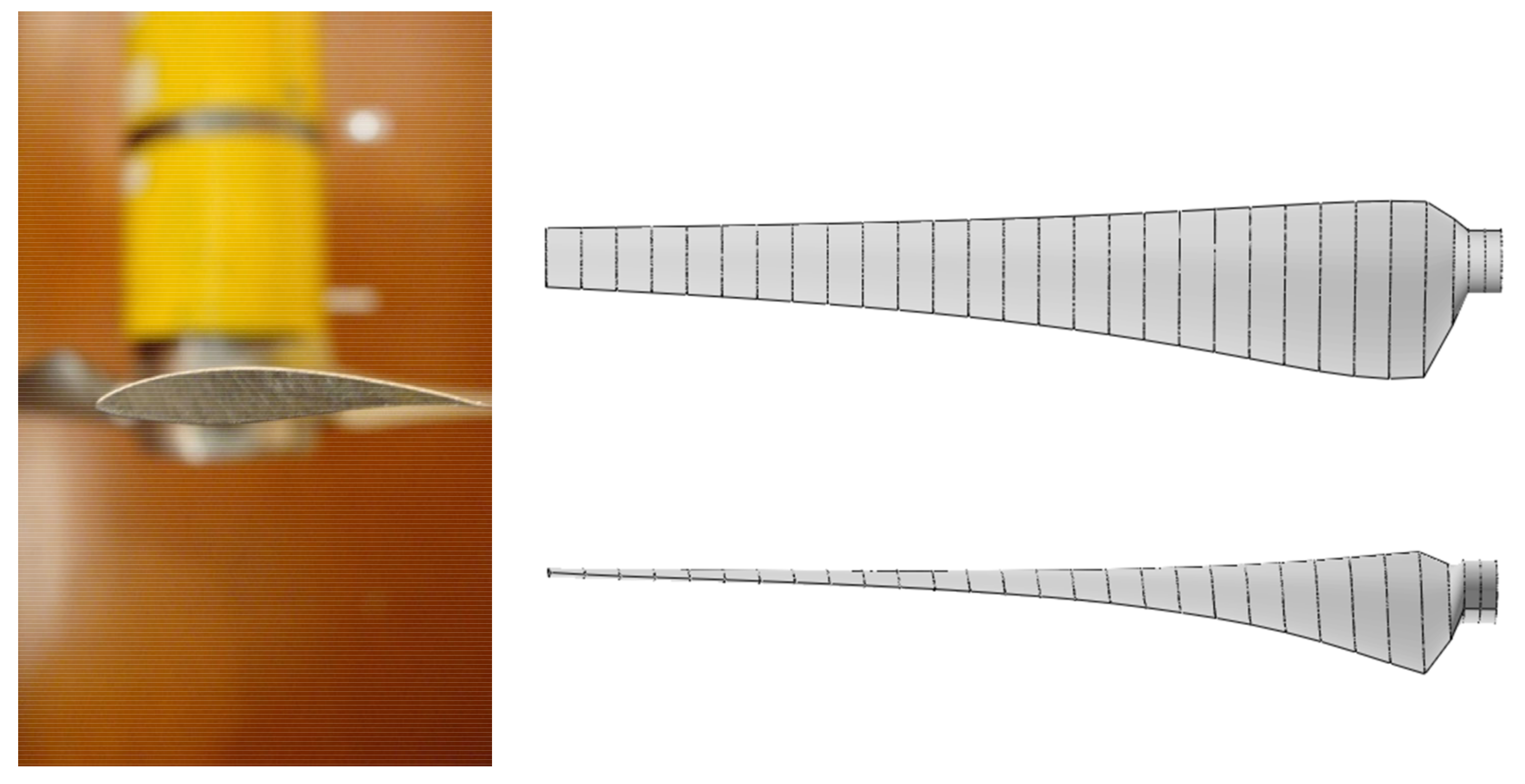
2.1. Experimental Setup

In the present experimental campaign, the upstream turbine is denoted as “T1”, while the downstream turbine (in the aerodynamic wake) is “T2”. The blades used in both turbines are the same, but due to different hub geometries, the overall rotor diameters differ slightly: DT1 = 0.944 m and DT2 = 0.894 m. The basic dimensions of the test setup are presented in Figure 2.

DT1 = D is reference dimension, used for denoting the dimensionless distance between turbines x/D. Therefore, x/D = 0 denotes the T1 position, located approximately 2D from test section inlet. The wind turbines’ performance was assessed for wind turbine separation distances of 2.63D, 4.90D and 8.52D, referred to, respectively, as cases 2.5D, 5.0D and 8.5D. Additionally, the T1 wake was measured at vertical and horizontal lines, as seen in Figure 2 (case 7.5D collected at x/D = 7.58, case 8.0D at x/D = 8.05). Note that the horizontal line data at locations 2.5D, 5.0D and 7.5D were collected in the absence of T2.

Both turbines were equipped with AC generators of 0.37 kW power, controlled by a frequency converter SIEMENS Micromaster440. This provided a precise regulation of rotational velocity (with an accuracy of around 3–6 rpm), up to 3000 rpm. The measurement of rotor speed was realized by an optical sensor, mounted inside of the nacelle. The control system maintained the given rotational velocity and transmitted the generated electrical energy to the 300 W receiver (load). The generators were placed outside of the nacelles, and the mechanical power was transferred through the flat belt transmission. The overall view of the test section ready for the test is presented in Figure 3.

The blades of both wind turbines were designed employing NREL S826 airfoil (see Figure 4). This profile, one of the most popular ones for small wind turbine blades, has been thoroughly investigated by many research centres. Somers [37] examined S826 in the range of Re = 1.0·10⁶ to Re = 3.0·10⁶. Sarmast et al. [38] tested two-dimensional S826 in the range of Re = 0.4·10⁵ to Re = 1.2·10⁵ (experiment and simulation). Sarlak et al. [39] characterized the flow around the profile at Re = 1.0·10⁵. Another set of data was collected by Ostovan et al. [40], with drag and lift coefficients determined for the Reynolds number range from 0.72·10⁵ to 1.45·10⁵. The most recent characteristics were collected by Bartl et al. [41], in the range of Re = 0.5·10⁵ to 6.0·10⁵. These results are presented in Figure 5. One can notice a stable (i.e., devoid of abrupt changes) behaviour of the profile according to C_L and C_D coefficient characteristics for Re > 0.7·10⁵. Below that value, there is a significant decrease in the airfoil’s performance: lift force is reduced for the operating range and pre-stall conditions are observed at lower α (as low as 10°).

In the analysed case, for a wind turbine working at its optimal point, the local Reynolds number at the blade tip varies from Re = 0.8·10⁵ (for λ = 4) to 1.3·10⁵ (λ = 7). The maximum achievable lift coefficient is obtained at α between 12° and 14°—for higher α, the stall occurs. As seen in Figure 5, for Re values 1.0·10⁵ and higher, the airfoil characteristics’ dependence on the Reynolds number is minor (except perhaps for the drag at pre-stall conditions, which is not the most significant from the point of view of the current study). This information proves that the conclusions derived in the present study may not only be applied for small wind turbines, but may be scaled up for bigger machines, operating normally at relatively higher Reynolds numbers.

2.2. Wind Tunnel Equipment

The test section of the NTNU wind tunnel is 2.71 m wide and 11.15 m long, with an adjustable roof to ensure zero pressure gradient and maintain constant freestream velocity along the whole test section. The test section hosts an automatic traverse (three-axis, used for the single wind turbine tests) and a manual one (one-axis (vertical), having smaller blockage for measurements in the aerodynamic wake of T1). Both traverses enable mounting pressure probes, thermocouples and CTA probes.

All presented data were collected during measurement sessions performed at the freestream velocity U_∞ ≈ 11.5 m/s. T1 and T2 performance (rotational velocity ω, torque Q), aerodynamic force (force F_x) and flow properties in selected positions in the aerodynamic wake of T1 were measured, at two different inlet conditions: low turbulence intensity (IT ≈ 0.23%) and high turbulence intensity (IT ≈ 10.00%). The presented values of U_∞ and IT are the average ones at location x/D = 2 (i.e., rotor plane of T1). The abovementioned low turbulence intensity is the nominal value for the NTNU wind tunnel, and the maximal single IT value recorded at the empty test section measurements did not exceed 0.50%. The average values of turbulence intensity recorded by other researchers vary normally from IT = 0.23% [42] to IT = 1.00% [26].

To obtain the high turbulence intensity, a turbulising grid was employed. According to Pope [43], a grid of appropriate geometry can generate vortex structures of uniform dimensions, resulting in increased overall turbulence intensity. Krogstad and Davidson [44] determined that the generated turbulence reaches uniformity at the distance corresponding to x/D = 2 in presented research. The turbulising grid was made of wood and covered the whole wind tunnel cross-section (2.7 m × 1.8 m). The wood slats of width 0.48 m resulted in square-shaped slots of size 0.192 m × 0.192 m. The solidity ratio of the grid was equal to σ = 35%, with a drag coefficient of CD ≈ 2.0.

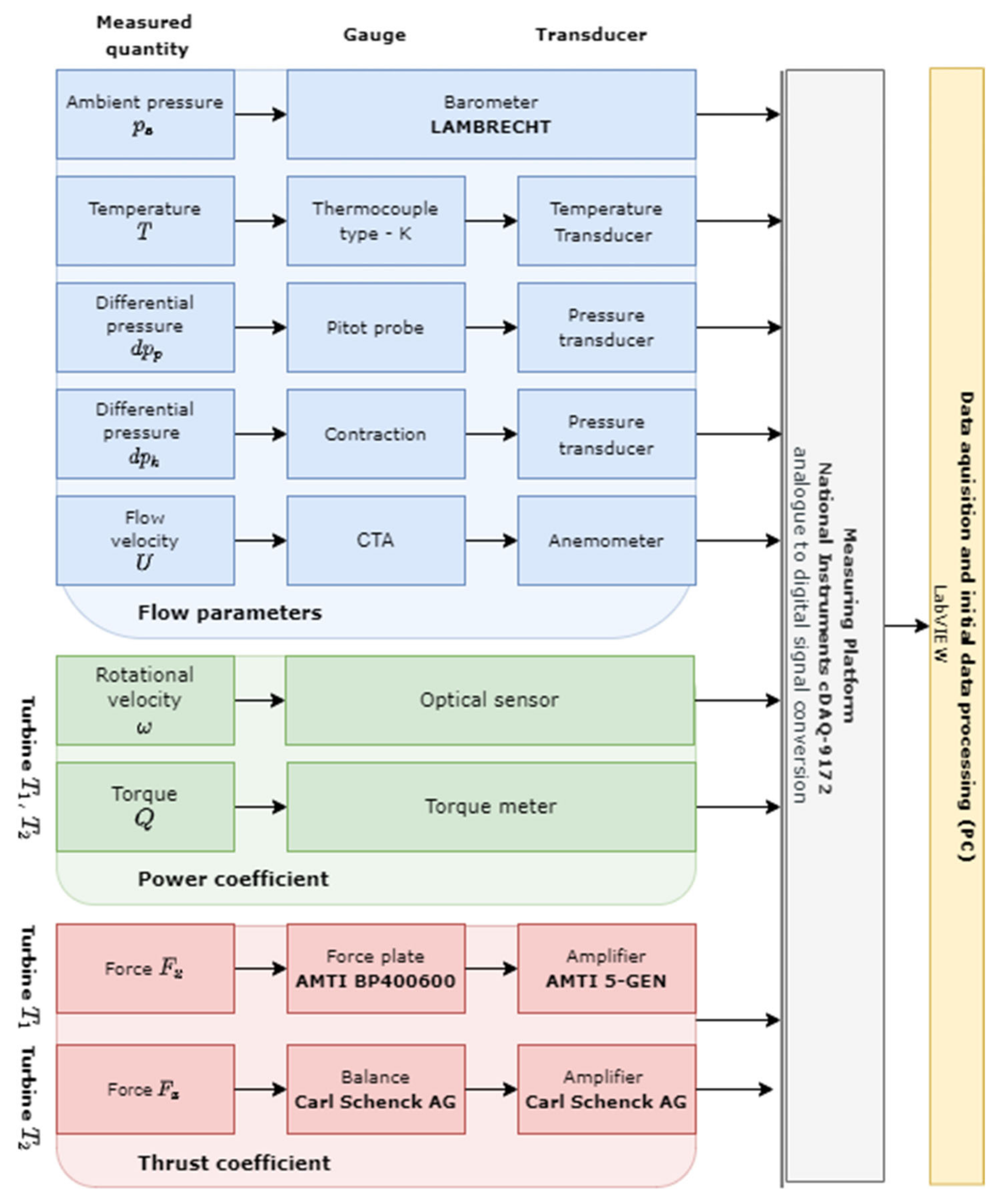
2.3. Measured Quantities

The schematic diagram of measured quantities and measurement devices is presented in Figure 6. The wind turbine performance may be normalised using coefficients of power (Cp) and thrust (Ct). Shaft torque Q, rotor thrust force F_x and its rotational velocity ω are measured, along with the reference, freestream velocity U_∞. The generated power can be calculated as P = ω · Q. Coefficients of power (Cp) and thrust (Ct) are evaluated, as seen in Formulas (1) and (2). Additionally, the rotational speed is normalised in the form of tip speed ratio λ = (ω · r)/U_∞.

$$\mathrm{Cp}=\frac{{\mathrm{P}}_{\mathrm{rotor}}}{{\mathrm{P}}_{\mathrm{wind}}}{=4\mathrm{a}(1-\mathrm{a})}^2$$

(1)

$$\mathrm{Ct}=\frac{{\mathrm{F}}_{\mathrm{T}}}{{\mathrm{F}}_{\mathrm{Twind}}}=4\mathrm{a}(1-\mathrm{a})$$

(2)

where a = 1 − (U_R/U_∞) is the axial induction factor, with U_R—flow velocity in rotor plane.

3. Results

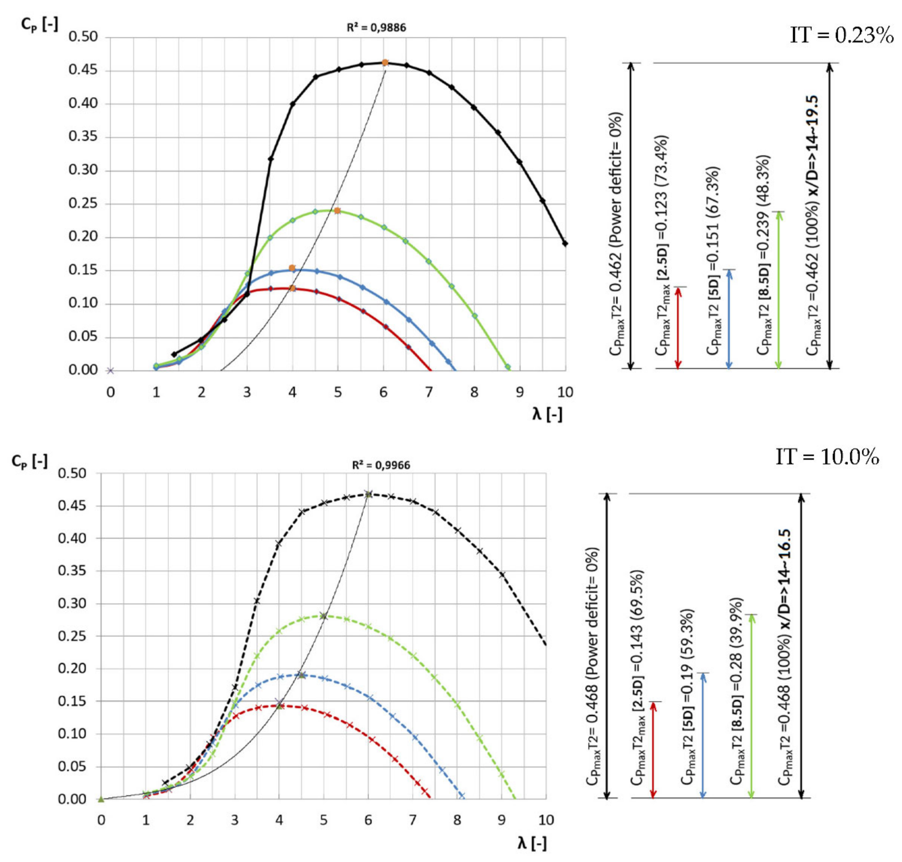
3.1. Single Turbine’s Independent Operation (No Interaction)

Initial measurement sessions were performed for both wind turbines working in isolation (T1 with T2 dismounted and T2 with T1 dismounted). Both turbines were tested at location 2D from the inlet with low IT (0.23%) and high IT (10.0%). Power coefficient as a function of tip speed ratio for T2 is presented in Figure 7. For both turbines, the increase of IT at the test section inlet results in increased efficiency. Furthermore, for high IT, the Cp values are globally higher, notably in the range of λ between 3 and 4. The maximum Cp is also acquired at a slightly higher tip speed ratio.

3.2. Velocity Profiles between the Turbines

Figure 8 presents the vertical profiles of the velocity deficit and turbulence intensity in the flow downstream T1. For x/D = 2.5, 5.0 and 7.5, the data were collected in tandem operation. Since the measurement location x/D = 7.5 was just in front of the working T2, the flow was observed to be influenced by the machine and partially blocked (see also Figure 9). The collected data was used to construct basic mathematical models according to different schemes (see, for example, the Jensen model [45]) to check their prediction of full velocity recovery. Velocity deficit is defined as

$$\begin{array}{c}\mathrm{Velocity} \mathrm{deficit}=\left(1-\frac{\overline{{\mathrm{U}}_{\mathrm{z}}}}{{\mathrm{U}}_{\infty }}\right), \left[\%\right] \hspace{1em}\mathrm{for} \hspace{1em}\mathrm{z}\in \left[-\mathrm{R},\mathrm{R}\right]\end{array}$$

(3)

The fastest recovery is achieved for the second order polynomial fitting (dashed) and linear fitting (solid), predicting the full recovery in the x/D range of 14 to 17; the exponential fitting (dotted line) asymptotic point is situated above x/D = 50. In general, the higher-level turbulence models propose faster velocity recovery, which may be attributed to the accelerated flow mixing. This is also supported by the observation of the velocity profiles (Figure 8), in which the higher-turbulence velocity field becomes smoother more rapidly than in case of IT = 0.23%. It is also worthy of note that the vertical distributions of the flow velocity are slightly influenced by the presence of the wind turbine tower and the downwash effect and hence lack symmetry with respect to the axis of rotation.

Figure 10 presents the horizontal profiles of the velocity deficit and turbulence intensity in the flow downstream T1. Once again, the collected data were used to construct mathematical models (Figure 11). The fastest full velocity recovery is again predicted by the second order polynomial fitting (x/D between 11 and 13, dashed lines), followed by linear fitting (x/D approx. 17, solid line) and exponential fitting (dotted line, asymptotic point again situated above x/D = 50).

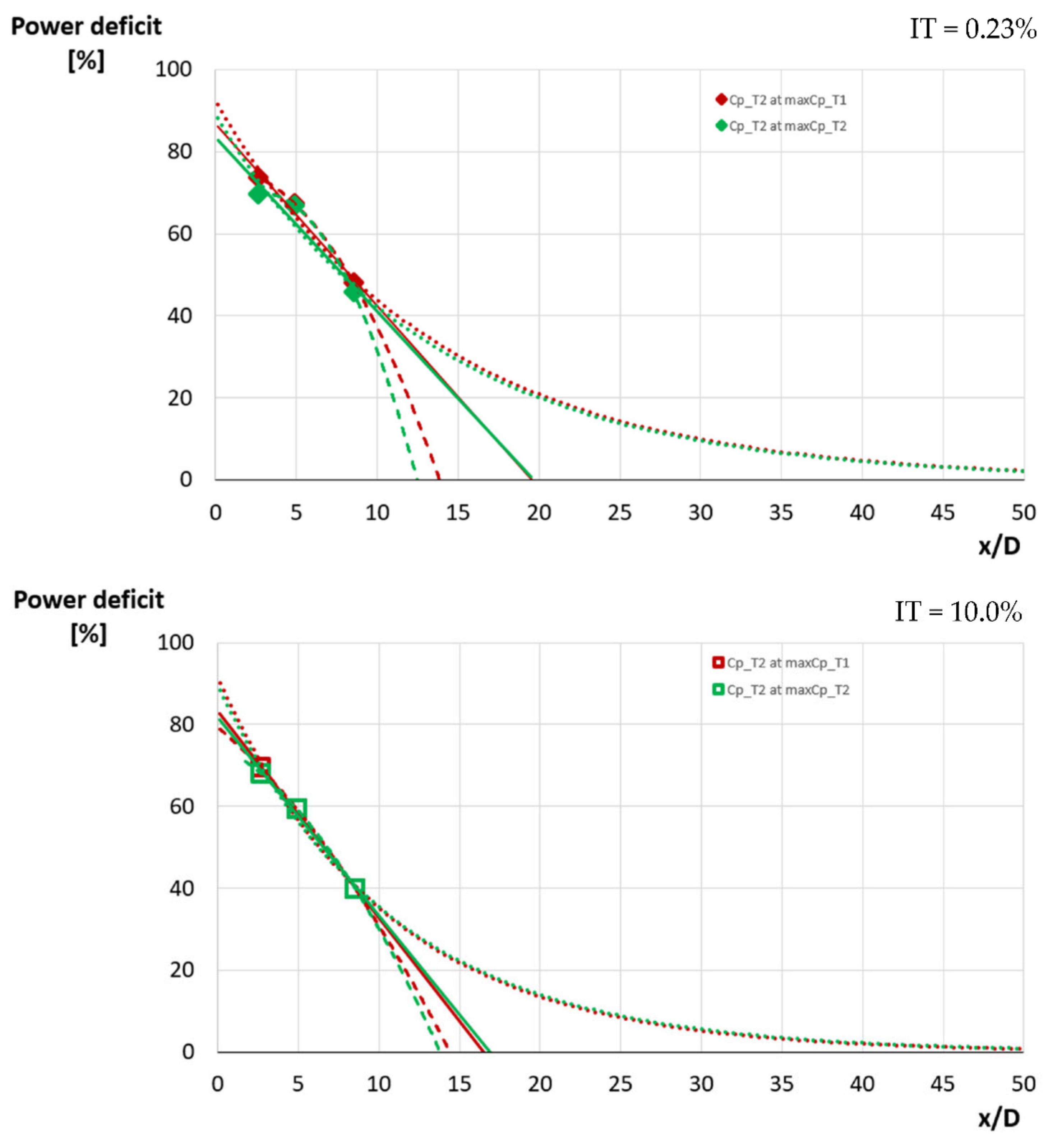
3.3. Determination of Efficiency for Two Turbines in “Tandem” Configuration

Two-dimensional charts describing the ratio between sum of power coefficients for T1 and T2 turbines and the sum of maximal power coefficients of isolated turbines (see (4)) are presented in Figure 12. The lowest presented values of total efficiency are at the level of 50%—all operation points below that value (not marked in the charts) correspond to the combination of tip speed ratios resulting in a performance lower than that obtained by a single turbine.

$$\mathsf{\eta } =\frac{\mathrm{Cp}\_\mathrm{T}{1}_{\mathrm{Tan}\mathrm{dem}(\max )}+ \mathrm{Cp}\_\mathrm{T}{2}_{\mathrm{Tan}\mathrm{dem}(\max )}}{\mathrm{Cp}\_\mathrm{T}{1}_{\left(\max \right)}+ \mathrm{Cp}\_\mathrm{T}{2}_{(\max )}}$$

(4)

The collection of data for all measurement points was performed with an assumption of fixed T1 working conditions while varying T2 tip speed ratio. Three distances between rotor planes T1 and T2 were investigated. For each operation point, the data were time-averaged.

Table 1. T1 and T2 operation points at which the total Cp (Cp_Sum) is maximized.

x/D	IT (%)	λ_T1	Cp_T1	λ_T2	Cp_T2	Cp_Sum	Cp Percentage Difference (%)
2.5	0.23	6.0	0.4671	3.5	0.1231	0.5902	0.03
		6.0	0.4665	4.0	0.1235	0.5900
	0.23	6.5	0.4644	3.5	0.1187	0.5831	0.06
		6.5	0.4636	4.0	0.1192	0.5828
	10.0	6.5	0.4766	3.5	0.1398	0.6164	0.11
		6.5	0.4734	4.0	0.1423	0.6158
5.5	10.0	8.0	0.4289	4.0	0.1956	0.6245	0.82
		8.0	0.4205	4.5	0.1990	0.6194
8.5	0.23	6.5	0.4747	4.5	0.2393	0.7140	0.07
		6.5	0.4742	5.0	0.2393	0.7135
	0.23	7.0	0.4598	4.5	0.2422	0.7020	0.09
		7.0	0.4600	5.0	0.2414	0.7014
	0.23	8.0	0.4089	4.5	0.2604	0.6693	0.18
		8.0	0.4074	5.0	0.2607	0.6681

presents the selected results: T1 and T2 operation parameters that result in maximisation of the total set efficiency (Cp_Sum = Cp_T1 + Cp_T2); in each case the two highest Cp_Sum results are shown. Cp percentage difference is the absolute difference divided by the average value of the two compared Cp values.

4. Discussion

4.1. Individual Turbines, No Interaction

The maximum efficiencies obtained by isolated wind turbines for two levels of inlet turbulence intensity are presented in

Table 2. Maximum Cp for isolated wind turbines.

	IT = 0.23%	IT = 10.0%
T1	0.477	0.481
T2	0.462	0.468

. One can observe, for both T1 and T2, a higher maximum power coefficient for the increased value of IT. Due to the differences in hub diameter and design of the tower, T2 achieves slightly better efficiency under both inlet turbulence values. On the other hand, increasing turbulence intensity results in shifting the highest Cp regions of turbine operation towards higher tip speed ratios (from around λ = 5.5 to λ = 6). The plateau of optimum operation is also wider at increased IT, meaning that the turbine performance is less prone to variations of tip speed ratio (see Figure 7). This allows us to conclude that the increase in turbulence intensity makes the airfoil less dependent on the Reynolds number variations (see Figure 5), which can be associated with the forced boundary layer turbulisation at higher IT flow, causing in turn more stable and favourable operation of the wind turbine [46]. Thus, the turbulence intensity influence may be related to the aspect of stability of the flow at the individual sections of the blade (see, e.g., [47]).

4.2. Two Turbines, Inlet Turbulence Intensity Influence

Possibly the most straightforward conclusion concerning the interdependence of the turbine performance is the fact that for the optimal working point of T1 (maximum T1 Cp), the T2 performance drops. The power coefficients of both turbines are inversely related due to the conservation of energy principle. The increase of distance between T1 and T2 results in globally higher T2 efficiency values. The shape of the T2 power coefficient curve is also less influenced by T1 operation as the turbines are moved apart.

The increase of the flow turbulence intensity results in diminishing of the differences between minimum and maximum power produced by T2. The optimal operation range of λ_T2 is from approximately 3.5 to 5. Notably, lower values are preferred for lower separation between the turbines: for x/D = 2.5 and 5.0, the most favourable values of λ_T2 are in range 3.5–4.5; for x/D = 8.5, it is λ_T2 = 5. The importance of the distance between T1 and T2 and optimal λ_T2 becomes more clear at higher IT: the optimal tip speed ratio of T2 for x/D = 2.5, 5.0 and 8.5 is, respectively, λ_T2 = 4, 4.5 and 5.

The collection of maximum values of total power coefficients is presented in

Table 3. Summary of characteristic points of turbine tandem operation (red—maximum Cp_T1, green—maximum Cp_T2, bold blue—maximum Cp_Sum).

x/D	IT (%)	λ_T1	Cp_T1	λ_T2	Cp_T2	Cp_Sum	Cp Percentage Difference (%)
2.5	0.23	4.5	0.4528	4.0	0.1398	0.5927	0.42
		6.0	0.4671	3.5	0.1231	0.5902
	10.0	5.5	0.4739	4.0	0.1490	0.6229	0.48
		6.0	0.4772	4.0	0.1427	0.6199
5.0	0.23	6.0	0.4763	4.0	0.1512	0.6274	0.13
		6.5	0.4748	4.0	0.1534	0.6282
	10.00	-	-	-	-	-	-
		6.0	0.4799	4.5	0.1903	0.6701
8.5	0.23	5.0	0.4698	5.0	0.2505	0.7203	0.47
		6.0	0.4771	5.0	0.2398	0.7169
	10.00	-	-	-	-	-	-
		6.0	0.4805	5.0	0.2811	0.7615

. Red colour denotes the highest values of Cp_T1 (all occur at the nominal operation point for T1, namely at λ_T1 = 6). Green colour denotes the highest obtained values of Cp_T2, which also result in the highest Cp_Sum. For four out of six cases (except for IT = 10.0% and distances x/D = 5.0 and x/D = 8.5), the maximum obtained total power was obtained at non-optimal T1 operating conditions. The percentage increase of total power coefficient is presented in the rightmost column.

One can conclude that it is more profitable to ensure the operation of the upstream turbine at a lower- or higher-than-optimal tip speed ratio. This would enable the subsequent machine to gain more energy from the perturbed flow, eventually resulting in higher total power production of a whole wind farm. Wind farms are designed to avoid frequent turbine shadowing, but excluding this effect completely is impossible. While the efficiency gain in itself is not impressive, the wind turbine’s significant operation time under the concerned conditions translates into a noteworthy profit. Lastly, it is also important to note that in real-life conditions, the flow between turbines is additionally repowered by the ambient free stream, which cannot be emulated in the current, closed-loop wind tunnel results.

The visible tendency in increase of Cp obtainable by T2, along with extending the distance behind the T1 turbine, allows the estimation of minimum displacement at which the second turbine would operate similarly to the freestream conditions (Cp_maxT2 in both graphs in Figure 13). Such estimation is presented in Figure 13 and Figure 14. The Cp characteristics for different x/D (2.5, 5.0, 8.5) in Figure 13 are supplemented with a curve for isolated T2 turbine performance. For IT = 0.23% (Figure 13, top), the available Cp_maxT2 = 0.48 can be reached if the distance between the turbines is to be approximately x/D = 14 to x/D = 19.5. In case of IT = 10.0% (Figure 13, bottom), Cp_maxT2 = 0.49 is predicted to be obtained at x/D in range from 14 to 16.5.

The obtained Cp_T2 data were used to construct power deficit, defined as

$$\mathrm{Power} \mathrm{deficit}=\left(1-\frac{{\mathrm{Cp}}_{\mathrm{T}2}{}_{\mathrm{i}}}{{\mathrm{Cp}}_{\mathrm{T}2}{}_{\max }}\right), \left[\%\right]$$

(5)

where subscript “i” refers to the maximum power coefficient in a particular x/D, while “max” is global maximum, for undisturbed T2. In Figure 14, modelling of the power recovery was done using the same models as in Figure 9 (dashed line—second order polynomial; continuous line—line fit; dotted line—exponential model). The second order polynomial fits predict the earliest full recovery of the power, after approximately 13 to 14 diameters downstream T1, similar to IT = 0.23% and 10.00%. This, along with the linear fit (full power recovery approximately 17 to 19 diameters downstream T1), seems to be the most appropriate distance to be considered if full recovery of the available power is desired. Other researchers estimated the distance as a displacement of x/D = 20 to even x/D = 30 [48]. The current study puts this value at much lower levels, with an additional annotation that the study was done in a closed test section, which makes the flow recovery even more difficult.

4.3. Applicability of Findings

The highest tandem system efficiency (defined by (4); see Figure 12) observed in the tests was η = 81% (at x/D = 8.5 and IT = 10.0%). At the other end of the spectrum, at x/D = 2.5 and IT = 0.23%, the efficiency was equal to η = 64%. It may be said that in the former case, both T1 and T2 experienced high IT (T1 owing to the flow character, T2 additionally due to operation in the T1 wake), while in the latter—only T2 experienced high turbulence. It is also worth noticing that the tandem system operating region (of relatively highest η) was obtained at a plateau for a wide range of consecutive rotor TSR. This means that high performance of the system can be preserved despite some perturbations of tip speed ratio of any of the machines, which is beneficial from the practical point of view, as ensuring a strict value of TSR is a challenging task in real-life operating conditions. It should be noted that the described effect was more pronounced for the high turbulence intensity.

The considerable influence of TSR and IT on the wind turbine performance can be confronted with the research on full-scale wind farms. It is difficult to assess the exact extent of aerodynamic wake influence on a wind turbine in field conditions due to the relative scarceness of in situ measurement data. Nonetheless, we decided to compare our research findings with full-scale wind farm operations, where the turbines are placed in line [49,50]. Figure 15 aggregates these data, with the wind turbine efficiencies normalized using nominal values for respective machines. In the case of Lillgrund wind farm, the wind turbine localised in a wake of the first-in-row (at the distance x/D = 3.3) operates at only 30% of normal efficiency, and the subsequent machines work with an efficiency not higher than 40%. The wind farms with distance between the turbines of x/D = 7.0 (Horns Rev) and x/D = 10.3 (Nysted) present a similar performance (in particular for the first four turbines in a row). All turbines (except the one exposed to the freestream) work with efficiencies slightly above 60%. For all three wind farms, the significant drop in performance is noted for the second turbine in line; the remaining ones have the efficiency stabilized at the level dependent on the distance between them.

Another important aspect required to be characterised in the context of turbines operating in a wind farm is the relation between the overall farm efficiency and its size. Figure 16 depicts the relation between the accumulated, theoretical power as a function of wind farm size (denoted as an x/D distance). Assuming a fixed number of wind turbines (eight in the presented example), one can compare the achievable power for a series of turbines.

Under the assumption that all turbines except the first in a row work with similar efficiency, it is visible that the highest performance from the tested combinations (next to Horns Rev and Nysted wind farms) can be achieved by a setup of turbines displaced by x/D = 9, operating at high turbulence intensity. In addition, the Horns Rev case seems most profitable, as a similar value of power is achieved at a relatively shorter total distance. On the other hand, increasing the number of turbines with the setup following x/D = 5 at high IT could result in a competitive result. Finally, it is important to remember that in the current research, the wind turbines are working in the worst possible layout, i.e., the downstream wind turbine is directly in the wake of the upstream rotor.

As a general rule of thumb, we can state that, according to the presented results, the wind speed downstream a wind turbine and the available power should regain their freestream values in less than x/D = 20, possibly closer to an x/D between 15 and 17. These results are given in a range, since the models that we applied are based on the first and second order polynomial fitting, which, nonetheless, both offer similar results and prove their applicability to this particular problem. Determining the precise coefficients for the models remains, however, a very individual, case-dependent aspect. Future studies and a more extensive experimental database may determine the repeatability and generality of such empirically-determined coefficients.

5. Conclusions

There are numerous factors influencing the efficiency of a wind farm. Along with changes of the direction of the wind, the fixed grid of wind turbines in a wind farm may be often subjected to unfavourable conditions, resulting in a drop of overall efficiency. Optimization of a grid of wind turbines by determining the minimum distance between the units (influencing both the size of a farm and the number of units) can lead to a significant increase of the total generated power and decrease the negative impact of operation in an aerodynamic wake. What can be concluded from research presented above is that the minimal distance at which the downstream turbine could be located to permit a non-disturbed operation is an x/D between 15 and 17. This would ensure the second-in-row turbine to operate in freestream-like conditions. Nevertheless, the precise power coefficient values of turbines are influenced strongly by environmental conditions and natural flow mixing.

In the current research, the experimental investigation of two turbines (the downstream one placed in the wake of the upstream one) enabled us to inspect the behaviour of the flow and its development along with the distance increase. The velocity deficit is reduced as the T1 wake mixes with the undisturbed flow. What enhances the mixing and re-organizes the flow is the increase of turbulence intensity. In a natural environment, this may be provoked by natural wind gusts or changes in the wind inflow conditions. Increased levels of turbulence intensity enlarge the plateau of optimum wind turbine operation; this results in the turbine performance being less prone to variations of tip speed ratio. From the applicational point of view, such a behavior is desirable, as ensuring a strict, optimal value of TSR in a narrow range is a challenging task in real-life operating conditions, especially in the case of a farm of turbines.

Another important conclusion is the profitability of ensuring the operation of the upstream turbine at a non-optimal tip speed ratio. This can permit the subsequent machine to gain more energy from the wake flow, eventually resulting in increased total power production of a whole wind farm. Thus, all power output maximisation analyses of wind turbine layout in a cluster should encompass not only the locations and distances between the units but also their operating parameters. The intentional alteration of efficiency of wind turbines in the farm’s first row (by deliberate reduction of TSR) can result in sparing more kinetic energy for the machines in consecutive rows. The axial induction factor can be diminished through pitch or yaw control of the upstream turbines.

Finally, the economic analyses must include the assessment of obtainable cumulative power in relation to the farm size (both in terms of the area and number of units). The appropriate compromise (turbines displaced at optimal distances, amount of turbines, cost of turbines) should be carefully evaluated in advance. Meticulous analysis may result in a conclusion that the optimal distance can be purposely diminished (resulting in voluntarily decreased energy gain) only if one or more additional units can result in a total increase of profit of a whole wind farm.

References

1. European Comission. Communication from the Commission to the European Parliament, the Council, the European Economic and Social Committee and the Committee of the Regions: 20 20 by 2020—Europe’s Climate Change Opportunity; European Commision: Brussels, Belgium, 2008. [Google Scholar]
2. European Comission. Communication from the Commission to the European Parliament, the Council, the European Economic and Social Committee, the Committee of the Regions and the European Investment Bank: Clean Energy for All Europeans; European Comission: Brussels, Belgium, 2016. [Google Scholar]
3. European Parliament. Energy Policy: General Principles; European Parliament: Brussels, Belgium, 2021. [Google Scholar]
4. BP plc. BP Statistical Review of World Energy 2021; BP PLC: London, UK, 2021. [Google Scholar]
5. Edenhofer. Renewable Energy Sources and Climate Change Mitigation; Cambridge University Press: Cambridge, UK, 2011. [Google Scholar]
6. Emeis, S. Wind Energy Meteorology, 2nd ed.; Springer: New York, NY, USA, 2013; ISBN 978-3-642-30523-8. [Google Scholar]
7. Enevoldsen, P.; Permien, F.-H.; Bakhtaoui, I.; von Krauland, A.-K.; Jacobson, M.Z.; Xydis, G.; Sovacool, B.K.; Valentine, S.V.; Luecht, D.; Oxley, G. How much wind power potential does europe have? Examining european wind power potential with an enhanced socio-technical atlas. Energy Policy 2019, 132, 1092–1100. [Google Scholar] [CrossRef]
8. Lee, J.; Zhao, F. Global Wind Report 2021; Global Wind Energy Council: Brussels, Belgium, 2021. [Google Scholar]
9. World Wind Energy Association. Wind Power Capacity Worldwide Reaches 597 GW, 50.1 GW Added in 2018. 4 June 2019. Available online: https://wwindea.org/wind-power-capacity-worldwide-reaches-600-gw-539-gw-added-in-2018/ (accessed on 1 April 2022).
10. Veers, P.; Dykes, K.; Lantz, E.; Barth, S.; Bottasso, C.L.; Carlson, O.; Clifton, A.; Green, J.; Green, P.; Holttinen, H.; et al. Grand challenges in the science of wind energy. Science 2019, 366, eaau2027. [Google Scholar] [CrossRef] [PubMed] [Green Version]
11. Mosetti, G.; Poloni, C.; Diviacco, B. Optimization of wind turbine positioning in large windfarms by means of a genetic algorithm. J. Wind Eng. Ind. Aerodyn. 1994, 51, 105–116. [Google Scholar] [CrossRef]
12. Folkecenter for Renewable Energy. Catalogue of Small Wind Turbines (Under 50 kW); Folkecenter Print: Hurup Thy, Denmark, 2016. [Google Scholar]
13. Méchali, M.; Barthelmie, R.; Frandsen, S.; Jensen, L.; Réthoré, P.-E. Wake effects at Horns Rev and their influence on energy production. In Proceedings of the European Wind Energy Conference & Exhibition EWEC 2006, Athens, Greece, 27 February–2 March 2006. [Google Scholar]
14. Cleijne, J. Results of Sexbierum Wind Farm: Single Wake Measurements; Instituut voor Milieu- en Energietechnologie TNO: Apeldoorn, The Netherlands, 1993. [Google Scholar]
15. Neustadter, H.E.; Spera, D.A. Method for evaluating wind turbine wake effects on wind farm performance. J. Sol. Energy Eng. 1985, 107, 240–243. [Google Scholar] [CrossRef]
16. Bartl, J. Experimental Testing of Wind Turbine Wake Control Methods. Ph.D. Thesis, NTNU, Trondheim, Norway, 2018. [Google Scholar]
17. Elliott, D. Status of wake and array loss research. In Proceedings of the 21. American Wind Energy Association Conference Windpower ′91, Palm Springs, CA, USA, 24–27 September 1991. [Google Scholar]
18. Hou, P.; Zhu, J.; Ma, K.; Yang, G.; Hu, W.; Chen, Z. A review of offshore wind farm layout optimization and electrical system design methods. J. Mod. Power Syst. Clean Energy 2019, 7, 975–986. [Google Scholar] [CrossRef] [Green Version]
19. Zawadzki, K.; Baszczynska, A.; Fliszewska, A.; Molenda, S.; Bobrowski, J.; Sikorski, M. Fatigue testing of the small wind turbine blade. Int. J. Mech. Eng. Robot. Res. 2022, 11, 269–274. [Google Scholar] [CrossRef]
20. Barber, S.; Chokani, N.; Abhari, R. Wind turbine performance and aerodynamics in wakes within wind farms. In Proceedings of the European Wind Energy Conference and Exhibition EWEC 2011, Brussels, Belgium, 14–17 March 2011. [Google Scholar]
21. Barthelmie, R.; Hansen, K.; Frandsen, S.; Rathmann, O.; Schepers, J.; Schlez, W.; Phillips, J.; Rados, K.; Zervos, A.; Politis, E.; et al. Modelling and measuring flow and wind turbine wakes in large wind farms offshore. Wind Energy 2009, 12, 431–444. [Google Scholar] [CrossRef]
22. Marmidis, G.; Lazarou, S.; Pyrgioti, E. Optimal placement of wind turbines in a wind park using Monte Carlo simulation. Renew. Energy 2008, 33, 1455–1460. [Google Scholar] [CrossRef]
23. Johnson, K.E.; Thomas, N. Wind farm control: Addressing the aerodynamic interaction among wind turbines. In Proceedings of the 2009 American Control Conference, St. Louis, MO, USA, 10–12 June 2009; pp. 2104–2109. [Google Scholar] [CrossRef]
24. Adaramola, M.S.; Krogstad, P. Experimental investigation of wake effects on wind turbine performance. Renew. Energy 2011, 36, 2078–2086. [Google Scholar] [CrossRef]
25. Krogstad, P.; Adaramola, M.S. Performance and near wake measurements of a model horizontal axis wind turbine. Wind Energy 2011, 15, 743–756. [Google Scholar] [CrossRef]
26. Bartl, J.; Pierella, F.; Sætrana, L. Wake measurements behind an array of two model wind turbines. Energy Procedia 2012, 24, 305–312. [Google Scholar] [CrossRef] [Green Version]
27. Eriksen, P.E. Rotor Wake Turbulence: An Experimental Study of a Wind Turbine Wake. Ph.D Thesis, Norwegian University of Science and Technology, Trondheim, Norway, 2016. [Google Scholar]
28. Sætran, L.; Bartl, J. Invitation to the 2015 “Blind Test 4” Workshop: Combined Power Output of Two In-Line Turbines at Different Inflow Conditions; Norwegian University of Science and Technology: Trondheim, Norway, 2015. [Google Scholar]
29. Olasek, K.; Karczewski, M.; Lipian, M.; Wiklak, P.; Jozwik, K. Wind tunnel experimental investigations of a diffuser augmented wind turbine model. Int. J. Numer. Methods Heat Fluid Flow 2016, 26, 2033–2047. [Google Scholar] [CrossRef]
30. Lipian, M.; Czapski, P.; Obidowski, D. Fluid–structure interaction numerical analysis of a small, urban wind turbine blade. Energies 2020, 13, 1832. [Google Scholar] [CrossRef]
31. Stępień, M.; Kulak, M.; Jóźwik, K. “Fast Track” analysis of small wind turbine blade performance. Energies 2020, 13, 5767. [Google Scholar] [CrossRef]
32. Sobczak, K.; Obidowski, D.; Reorowicz, P.; Marchewka, E. Numerical investigations of the savonius turbine with deformable blades. Energies 2020, 13, 3717. [Google Scholar] [CrossRef]
33. Lipian, M.; Dobrev, I.; Karczewski, M.; Massouh, F.; Jozwik, K. Small wind turbine augmentation: Experimental investigations of shrouded- and twin-rotor wind turbine systems. Energy 2019, 186, 115855. [Google Scholar] [CrossRef] [Green Version]
34. Lipian, M.; Dobrev, I.; Massouh, F.; Jozwik, K. Small wind turbine augmentation: Numerical investigations of shrouded- and twin-rotor wind turbines. Energy 2020, 201, 117588. [Google Scholar] [CrossRef]
35. Krogstad, P.; Lund, J. An experimental and numerical study of the performance of a model turbine. Wind Energy 2011, 15, 443–457. [Google Scholar] [CrossRef]
36. Krogstad, P.; Sætran, L.; Adaramola, M.S. “Blind Test 3” calculations of the performance and wake development behind two in-line and offset model wind turbines. J. Fluids Struct. 2015, 52, 65–80. [Google Scholar] [CrossRef]
37. Somers, D. The S825 and S826 Airfoils; NREL: Golden, CO, USA, 2005. [Google Scholar]
38. Sarmast, S.; Mikkelsen, R.F. The Experimental Results of the NREL S826 Airfoil at Low Reynolds Numbers; Royal Institute of Technology in Stockholm (KTH): Stockholm, Sweden, 2012. [Google Scholar]
39. Sarlak, H.; Mikkelsen, R.; Sarmast, S.; Sorensen, J.N.; Chivaee, H.S. Aerodynamic behaviour of NREL S826 airfoil at Re = 100,000. J. Phys. Conf. Ser. 2014, 524, 012027. [Google Scholar] [CrossRef]
40. Ostovan, Y.; Amiri, H.; Uzol, O. Aerodynamic characterization of NREL S826 airfoil at low Reynolds numbers. In Proceedings of the Conference on Wind Energy Science and Technology—RUZGEM 2013, Ankara, Turkey, 3 October 2013. [Google Scholar]
41. Bartl, J.; Sagmo, K.F.; Bracchi, T.; Sætran, L. Performance of the NREL S826 airfoil at low to moderate Reynolds numbers—A reference experiment for CFD models. Eur. J. Mech. Eur. J. Mech. B/Fluids 2018, 75, 180–192. [Google Scholar] [CrossRef]
42. Ceccotti, C.; Spiga, A.; Bartl, J.; Sætran, L. Effect of upstream turbine tip speed variations on downstream turbine performance. Energy Procedia 2016, 94, 478–486. [Google Scholar] [CrossRef] [Green Version]
43. Pope, S.B. Turbulent Flows; Cambridge University Press: Cambridge, UK, 2000. [Google Scholar]
44. Krogstad, P.; Davidson, P.A. Is grid turbulence Saffman turbulence? J. Fluid Mech. 2009, 642, 373–394. [Google Scholar] [CrossRef]
45. Jensen, N. A Note on Wind Generator Interaction (Risø-M-2411); Risø National Laboratory: Roskilde, Denmark, 1983. [Google Scholar]
46. Zhang, Y.; Zhou, Z.; Wang, K.; Li, X. Aerodynamic characteristics of different airfoils under varied turbulence intensities at low reynolds numbers. Appl. Sci. 2020, 10, 1706. [Google Scholar] [CrossRef] [Green Version]
47. Talavera, M.; Shu, F. Experimental study of turbulence intensity influence on wind turbine performance and wake recovery in a low-speed wind tunnel. Renew. Energy 2017, 109, 363–371. [Google Scholar] [CrossRef]
48. Chamorro, L.P.; Porté-Agel, F. Effects of thermal stability and incoming boundary-layer flow characteristics on wind-turbine wakes: A wind-tunnel study. Bound. Layer Meteorol. 2010, 136, 515–533. [Google Scholar] [CrossRef] [Green Version]
49. Barthelmie, R.; Hansen, K.; Rados, K.; Schlez, W.; Jensen, L.E.; Neckelmann, S. Modelling the impact of wakes on power output at Nysted and Horns Rev. In Proceedings of the European Wind Energy Conference and Exhibition EWEC 2009, Marseille, France, 16–19 March 2009. [Google Scholar]
50. Gaumond, M.; Réthoré, P.-E.; Bechmann, A.S.; Ott, G.; Larsen, C.; Pena Diaz, A.; Hansen, K.S. "Benchmarking of wind turbine wake models in large offshore wind farms. In Proceedings of the Science of Making Torque from Wind 2012, Oldenburg, Germany, 9–11 October 2012. [Google Scholar]
Figure 1. Two turbines in a row—one-dimensional flow theory, based on [16].
Energies 15 03906 g001
Figure 2. T1 and T2 dimension overview (top, based on [36]) and measurement plane location of vertical profile conducted by manual traverse (middle) and in horizontal profile conducted by automatic traverse (bottom).
Energies 15 03906 g002aEnergies 15 03906 g002b
Figure 3. NTNU wind tunnel test section with two tested wind turbines.
Energies 15 03906 g003
Figure 4. NREL S826 airfoil profile (left); blade used in T1 and T2 turbines (right).
Energies 15 03906 g004
Figure 5. NREL Lift (CL, (a)) and drag (CD, (b)) coefficients vs. angle of attack (α) of NREL S826; experimental data for Re = 0.5·105 to Re = 6.0·105 [41] and Re = 1.0·106 [37].
Energies 15 03906 g005
Figure 6. Scheme of the measurement system.
Energies 15 03906 g006
Figure 7. Power coefficient curves for T2 turbine at low inlet turbulence intensity (solid red) and high inlet turbulence intensity (dashed blue).
Energies 15 03906 g007
Figure 8. Velocity deficit (top) and turbulence intensity (bottom) in the vertical plane between two turbines for x/D = 2.5, 5.0 and 7.5 and downstream T1 for x/D = 8.5. λ_T1 = 6.0 and λ_T2 = 5.0. High turbulence intensity inflow marked blue, low marked red.
Energies 15 03906 g008
Figure 9. Velocity deficit downstream wind turbines (vertical profile data): data points and their proposed modeling curves.
Energies 15 03906 g009
Figure 10. Velocity deficit (top) and turbulence intensity (bottom) in the horizontal plane downstream T1 for x/D = 2.5, 5.0 and 8.0. λ_T1 = 6.0. High turbulence intensity inflow marked blue, low marked red.
Energies 15 03906 g010
Figure 11. Velocity deficit downstream wind turbines (horizontal profile data): data points and their proposed modeling curves.
Energies 15 03906 g011
Figure 12. Total efficiency (in %) of two turbines.
Energies 15 03906 g012
Figure 13. Cp_T2 characteristics for x/D = 2.5 (red), 5.0 (blue), 8.5 (green) and T1 in reference conditions (undisturbed flow, no T2, black). In parentheses—Cp_T2 deficit with respect to the reference; x/D indicates the predicted distance for full power recovery (see also Figure 14). IT = 0.23% (top) and 10% (bottom). In tandem cases, λ_T1 = 6.
Energies 15 03906 g013
Figure 14. Power deficit and its recovery downstream T1 (λ_T1 = 6): data points and their proposed modeling curves. IT = 0.23% (top) and 10.0% (bottom).
Energies 15 03906 g014
Figure 15. Comparison of normalized power of two in-line turbines with full-scale wind farm performance: Nysted [49], Lillgrund and Horns Rev [50].
Energies 15 03906 g015
Figure 16. Comparison of cumulative power of eight full-scale turbines in Nysted [49], Lillgrund and Horns Rev [50] wind farms compared with current results (extrapolated).
Energies 15 03906 g016