Article

Exploratory Weather Data Analysis for Electricity Load Forecasting Using SVM and GRNN, Case Study in Bali, Indonesia

1
Generation Division, PLN Research Institute, Jakarta 12760, Indonesia
2
School of Computing, Telkom University, Bandung 40257, Indonesia
*
Author to whom correspondence should be addressed.
Energies 2022, 15(10), 3566; https://doi.org/10.3390/en15103566
Submission received: 30 March 2022 / Revised: 29 April 2022 / Accepted: 4 May 2022 / Published: 12 May 2022
(This article belongs to the Topic Artificial Intelligence and Sustainable Energy Systems)

Abstract

:
Accurate forecasting of electricity load is essential for electricity companies, primarily for planning electricity generators. Overestimated or underestimated forecasting value may lead to inefficiency of electricity generator or electricity deficiency in the electricity grid system. Parameters that may affect electricity demand are the weather conditions at the location of the electricity system. In this paper, we investigate possible weather parameters that affect electricity load. As a case study, we choose an area with an isolated electricity system, i.e., Bali Island, in Indonesia. We calculate correlations of various weather parameters with electricity load in Bali during the period 2018–2019. We use two machine learning models to design an electricity load forecasting system, i.e., the Generalized Regression Neural Network (GRNN) and Support Vector Machine (SVM), using features from various weather parameters. We design scenarios that add one-by-one weather parameters to investigate which weather parameters affect the electricity load. The results show that the weather parameter with the highest correlation value with the electricity load in Bali is the temperature, which is then followed by sun radiation and wind speed parameter. We obtain the best prediction with GRNN and SVR with a correlation coefficient value of 0.95 and 0.965, respectively.

1. Introduction

Electricity has become a vital part of the life of modern society nowadays. It is said that electricity access is an essential factor to enable the economic growth of a country or region [1]. Many studies also imply that the interruption of electricity supply has a severe impact on business and residential customers [2,3,4], where total electricity blackout can cost up to billions of dollars of economic activity [5]. These emphasize the importance of reliable and stable electricity supply to our current society.
One of the critical tasks in securing the electricity system’s reliability is maintaining the balance between electricity supply and demand. In current large power systems, the task is done by adjusting the power generated from generation units in the systems to a forecasted system electricity demand. Failure to do this correctly may cause the instability of the power system or even a blackout. On the other hand, low accuracy of electricity demand forecasting may also cause inefficient and costly operation of the generation units caused by the requirements of higher capacity of spinning reserve generators and lower efficiency of thermal generators [6]. The latter may also lead to higher carbon emissions which contribute to global temperature rises or global warming [7]. Inevitably, the accuracy of electricity demand forecasting is paramount in electric power system planning and operation.
There are two approaches for estimating energy use: statistical techniques and artificial intelligence [8]. In recent years, artificial intelligence has accelerated, with one of its applications being to improve the control of the current generation system. Predicting electrical loads for energy consumption is no longer a novel concept, as it can be accomplished through machine learning to predict future energy consumption points [9]. Numerous studies have been conducted because it is critical to understand the prediction of electrical energy consumption. For example, in 2018, Li and Zhang completed a short-term forecasting of electricity consumption in Shanghai by using grey prediction model [10]. Tian et al. predicted short-term electrical energy consumption using a combination model between STL (Seasonal and Trend decomposition using Loess) and GRU in the same year. They made predictions for the next 3 to 10 days using a combination model between STL (Seasonal and Trend decomposition using Loess) and GRU. When compared to GRU and SVM, GRU produces better results [11]. Hamdoun et al. projected electrical energy by comparing two different approaches, namely statistics and machine learning, to see more accuracy. They found that the prediction model based on machine learning produced the best results and had the lowest error rate among the findings they obtained [12]. Using a combination of the FPA (Flower Pollination Algorithm) model to optimize the Feedforward Neural Network (FNN), Zhao et al. made a short-term prediction of electricity consumption in 2020, then compared it with the SVR and RBFN models. The FPA-FNN model produced good results, with MAPE values of 1.41 percent and RMSE [13]. The Nonlinear Autoregressive (NARM) model was used to predict the electricity load for the next month for the energy management system in 2019. Ahmad and Chen then compared the NARM model to the Random Forest model and the linear model using stepwise regression in the case of ISO New England using the results obtained. They discovered that when compared to the other two models, the NARM model produced the best results [14].
Several studies have shown that weather parameters can affect the electricity load and need to be incorporated in power system planning and demand forecasting [15], both for short-term and long-term system planning [16]. Some studies evaluate the effect of weather parameters on the electricity system at regional and country levels, such as Algeria [17] and Turkey [18]. Other studies evaluated at a lower level, such as building electricity demand or residential house electricity consumption [19,20].
Aisyah and Simaremare investigate the correlation between weather parameters and electricity load in Bali by using three different weather source data, i.e., GFS, ERA5, and observation data from AWS (Automatic Weather Station) BMKG [21]. They conclude that three weather parameters are highly correlated with electricity load in Bali, i.e., temperature, wind speed, and solar radiation. This paper investigates which weather parameters affect electricity consumption in an isolated area by calculating the correlation coefficient with electricity load data. Bali has a significant increase in electricity consumption, and the Island does not have conventional resources [22], so it is crucial to estimate the electricity load for the future. That is by investigating which weather parameters affect most the electricity consumption. Additionally, to our best knowledge, no published research yet on the machine learning area was conducted for the electricity load forecasting in Bali. Thus, we chose Bali Island in Indonesia as a case study. Moreover, we also developed electricity load forecasting using two machine learning models: the Support Vector Regression (SVR) and the Generalized Regression Neural Network (GRNN), with weather parameter data and consumer characteristics as input for the machine learning models.
The SVM is one of the machine learning models that is usually used to solve regression and classification problems. It performs efficiently for time series prediction, especially for seasonal data [23]. Moreover, the SVM also effectively prevents overfitting problems by implementing Structural Risk Minimization (SRM) [24]. GRNN is simple to train and gives a satisfactory prediction, modeling, mapping, and interpolation [25,26]. It also performs efficiently for continuous data [27]. It has a higher learning speed than RBF [28]. To determine which weather parameters have the most significant effects on the electrical load, we create scenarios by gradually increasing the number of weather parameters used as features. Moreover, we also add scenarios in which moving average (MA) of electricity load data is used as a feature for the machine learning models. The innovations in this paper are as follows: firstly, we introduce a technique for feature selection from weather parameters, in which the selected features are used as the inputs to design machine-learning-based electricity forecasting. In [9,29], deep networks are used to make an electricity forecasting model, but they did not make feature selection for weather parameters. Secondly, weather parameters are used as features, but we also consider moving average (MA) data (daily, weekly, and monthly MA) as input for the machine-learning-based electricity load forecasting.
The content of this paper is as follows. Section 2 discusses electricity load data and some weather parameters in Bali and two machine learning models used. We discuss exploratory data analysis between weather parameters and electricity load data in Section 3. It is then followed by descriptions of obtained results and some discussions in Section 4. We conclude the paper in the final section.

2. Materials and Methods

2.1. Electricity Load Data
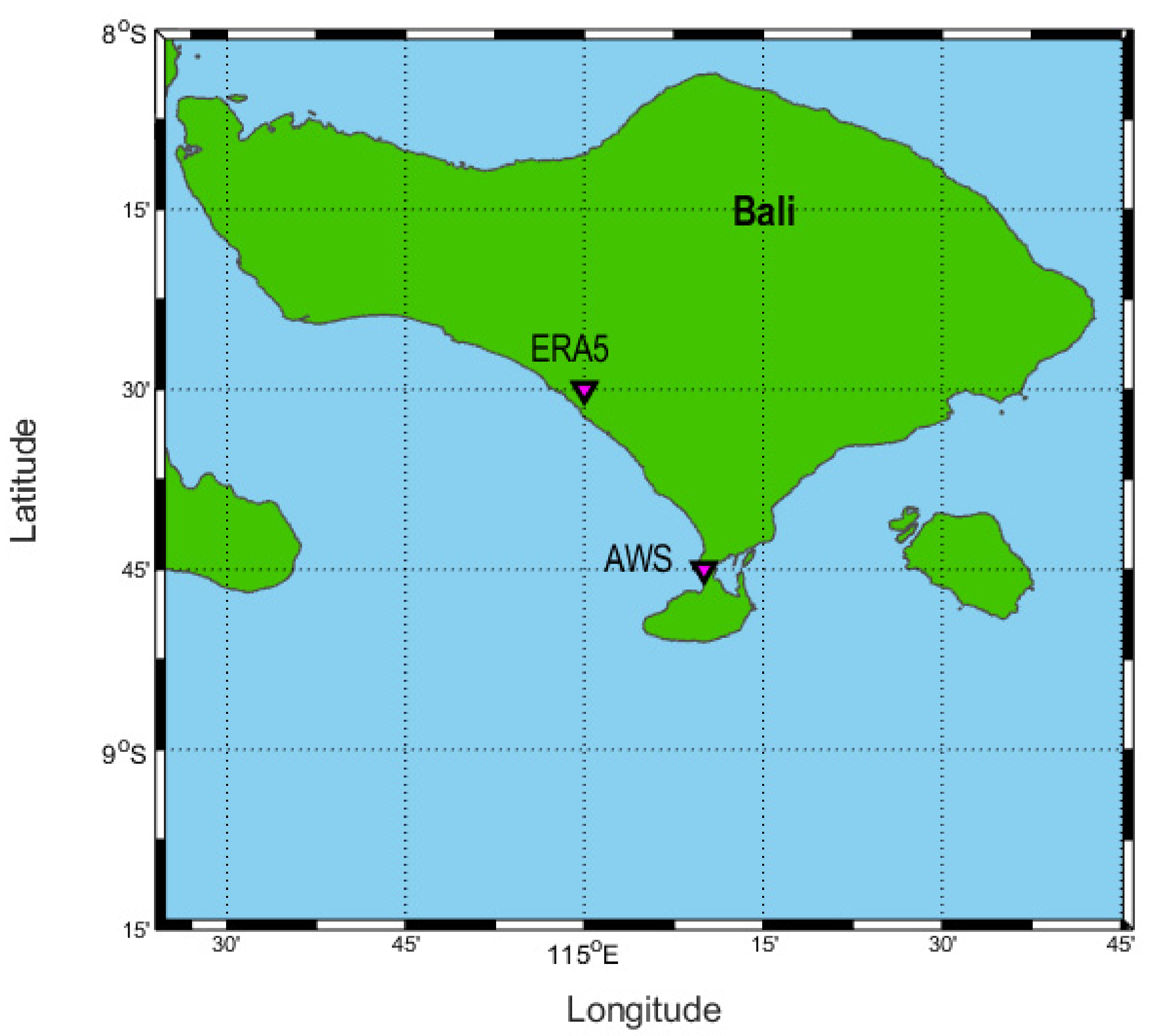
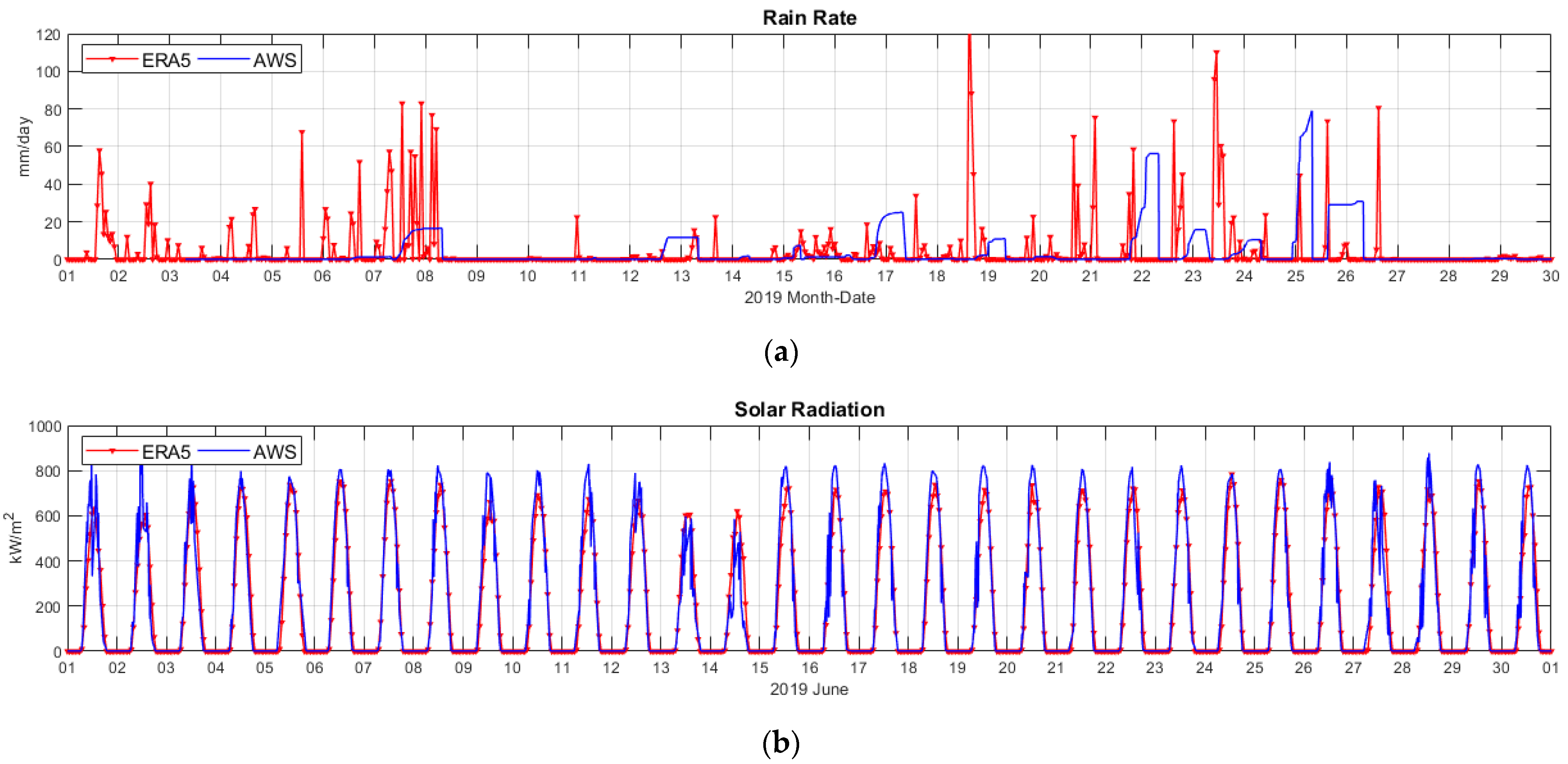
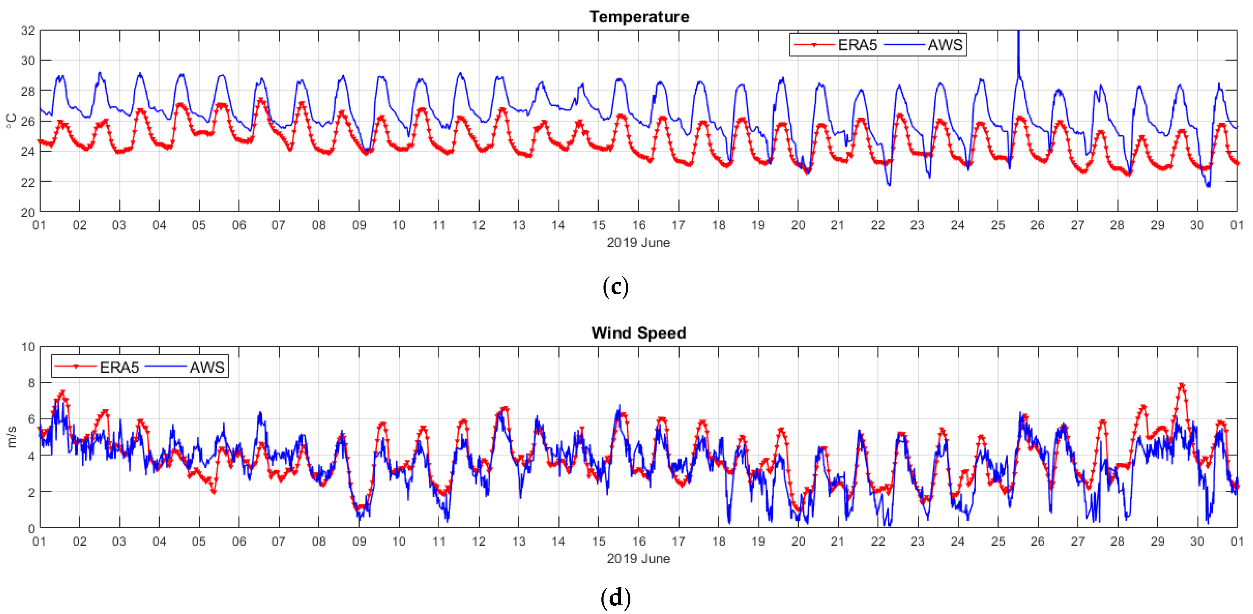
This study was conducted in a case study location with an isolated power grid system, i.e., Bali Island, located in Indonesia. Bali’s power is provided by external electricity producers from East Java Province and domestic electricity generators within the island. All of the power generated in Bali is utilized solely inside the island’s boundaries. As indicated in Figure 1, we are using two-year electricity load data, i.e., 2018–2019. As seen in Figure 1, the electricity demand in Bali follows a consistent pattern throughout the year, with peak demand occurring during January through May and September through November and peak demand occurring during June through August. According to Figure 1, there are anomalies in the power load statistics for both 2018 and 2019, namely, 17 March 2018, and 7 March 2019, which are both Nyepi Days in Bali, during which people in Bali refrain from engaging in any activity, indoor or outdoor, on those days. There was also an electricity interruption on 5 September 2018, which resulted in a total outage of electricity over the whole Bali islands. The daily averaged electrical load and the daily trend is also depicted in Figure 1, which was derived through linear regression. We may also assume from this trend line that the power demand increased from 2018 to 2019. On average, 0.123 megawatts (MW) per day are added to the daily trend line in 2018, and 0.162 MW per day is added to the daily trend line in 2019.
Not only is it vital to examine the yearly trend, but it is also critical to evaluate the daily and weekly variations of the power load in the system under investigation. Figure 2 depicts the weekly and daily variance in electricity demand in Bali for the year 2019. In terms of weekly variation, we can see in the left-hand portion of Figure 2 that the characteristics of electricity demand in Bali remain relatively constant during the weekdays. In contrast, on weekends, there is a slight decrease in electricity demand on Saturday and a slight decrease in electricity demand on Sunday. These features are unsurprising given that most people do not work on Sundays, resulting in decreased electricity demand. The lowest power consumption in Bali is at 4:00 a.m. local time, as seen in the right portion of Figure 2. Still, the highest electrical demand is between 8:00 and 10:00 a.m. local time, when people begin their activities during the day. During the lunch hour, between 12:00 and 01:00 p.m., when most individuals take their lunch break, there was a modest decrease in electricity demand. The most significant demand for power happened between 07:00 and 08:00 p.m. when individuals ate their dinner. These hourly and daily characteristics are crucial to consider when constructing an electrical load forecasting system. In the following subsection, we will discuss the weather data used in this work.

2.2. Weather Data

Primary weather data collected from field observations are the most optimal weather data to explain real-world weather conditions. While this fundamental data is somewhat inexpensive due to the requirement of a real-time measuring device, it is also highly costly. Furthermore, to use the observation data as a component of the energy load forecasting system, the observation data must be delivered to the forecasting system continuously, which necessitates the usage of a reliable measuring instrument. For this work, we will employ reanalysis weather data instead of real-time data as input for a machine learning model to be used as a feature in the electricity load forecasting system. This study uses the reanalysis weather data from the European Centre for Medium-Range Weather Forecasts, often known as the ECMWF, collected from the ERA5 model [30]. Since 1979, hourly weather data has been available, with spatial resolution varying between 0.25° and 0.75°. Weather parameters such as temperature, solar radiation, wind speed, rainfall rate, pressure, and relative humidity are investigated in this study.
To determine the quality of ERA5 weather parameter data, we compared the reanalysis data with observation data collected on Bali Island using an Automatic Weather Station (AWS) that has a temporal grid of 20 min. The AWS is positioned at latitude and longitude 115.167° E and 8.75° S. This study employs the most recent reanalysis ERA5 data from the nearest accessible grid to the AWS site, located at 115.00° E and 8.50° S, as shown in Figure 3. Indeed, the locations are quite a distance apart from one to another. Nonetheless, as seen in Figure 4, we compare many weather parameters from the ERA5 with the observed AWS data to identify any differences. We examine four meteorological factors: rainfall rate, solar radiation, temperature, and wind speed in Figure 4 during June 2019.
As shown in Figure 4, the solar radiation and wind speed, in particular, show a relatively similar trend between ERA5 and the observation data from AWS. In contrast, the other two parameters, i.e., the temperature and the rainfall rate, show a similar trend but with a different magnitude between ERA5 and the observation data from AWS. Because a significant distance separates the ERA5 point and the AWS point locations, this disparity might be caused by differences in local temperature and rainfall rates that are potentially highly different. The ERA5 data offers a good representation of the trend of meteorological parameters for Bali Island when compared to other data sources.

2.3. Methods

This paper has two main steps to design an electricity load forecasting system: (1) Exploratory data process to investigate correlations between weather parameters and electricity load; (2) Design a machine-learning-based model for electricity load forecasting using the best weather features obtained from step (1). For electricity load forecasting, two machine learning methods were utilized, namely, the Generalized Regression Neural Network (GRNN) and the Support Vector Regression (SVR) techniques (SVR). In the following subsections, we briefly describe these two methods.

2.3.1. Generalized Regression Neural Network

Donald F. Specht initially presented the General Regression Neural Network (GRNN) in 1991 [25], which is a deformation version of the radial basis function (RBF) neural network [28]. In comparison to RBF, GRNN improves at approximation and learning speed [31]. Its functioning is based on nonlinear or kernel regression, which implies that the result is dependent on the input. GRNNs may be utilized for prediction, modeling, mapping, and interpolation, as well as serving as controllers [25].
The GRNN architecture, as seen in Figure 5, is composed of four layers: the input layer, the pattern layer, the summation layer, and the output layer. The input layer takes and stores the input data Xi = [x1, x2, …, xn]. The number of neurons in a network is proportional to the amount of data input. The input layer’s result is then transmitted to the pattern layer. The pattern layer is nonlinear, and its neurons can retain information about the interaction between the input neurons and the pattern layer [31]. A pattern based on the Gaussian function Pi can be expressed as follows
P i   =   e x p X X i T   X X i 2 σ 2   i   =   1 ,   2 ,   ,   n
where σ is the smoothing or spreading parameter. The input variable is denoted by X, whereas xi denotes a more precise training sample from neuron i in the pattern layer.
Following the pattern, the summation layer performs two distinct computations referred to as numerators and denominators. The first kind is used to determine the number of weighted outputs from the pattern layer, whereas the second type is used to determine the number of unweighted outputs from the pattern layer [26]. The pattern layer’s purpose is as follows:
S s = i = 1 P i , i = 1 , 2 , , n
S w = i = 1 w i P i , i = 1 , 2 , , n
where S s is the denominator, S w is the numerator, and w i is the weight of the pattern neuron i connected to the summation layer.
The last layer is the output layer, the results of which are produced by dividing the neuron numerator S s by the neuron denominator S w . The output layer performs the following calculations:
y = S w S s
In comparison to other approaches, the primary advantage of GRNN is that it is simple to train and requires only one independent parameter [26]. GRNN does not require recurrent training and may be trained in a short period of time. While this is a disadvantage of GRNN over other algorithms, it does need significant processing to analyze new points. These shortcomings, however, can be solved by adopting the clustering version of GRNN or by executing computations using an embedded parallel structure and building a semi-conductor chip [25].

2.3.2. Support Vector Machine

Vapnik et al. pioneered the Support Vector Machine (SVM) in 1999 [32]. SVM is a classification and regression technique used in machine learning [23]. This technique is more effective when used in conjunction with Structural Risk Minimization (SRM) than when used in conjunction with Empirical Risk Minimization (ERM) [24]. Support Vector Regression is a machine learning model that allows for trade-offs between minimizing empirical errors and the complexity of the resultant fitted function, hence lowering the danger of overfitting [33]. SVR employs a soft margin approach to achieve the highest degree of generalization; the regression issue is handled using an alternate loss function and two slack variables [24]. As follows is the definition of the nonlinear regression problem using the SVR model.
y = f x = ω · ψ x + b
where ω is a weighted vector, b is a constant bias, and ψ x is the feature space mapping function. The following minimization procedure is used to obtain the coefficients of ω and b:
M i n i m i z e   1 2 w 2 + C 1 N i = 1 N ξ i + ξ i *
S u b j e c t   t o   y i w ,   x i + b     ε + ξ i w ,   x i + b y i     ε + ξ i * ξ i ,   ξ i *     0
where the parameters C and ε are model-defined. C evaluates the trade-off between empirical risk and smoothness, whereas 1 2 w 2 quantifies the function’s smoothness. ξ and ξ * are positive slack variables that indicate the difference between the actual and corresponding limit values in the approximation function’s ε -tube model.
Following the application of the Lagrangian multiplier and optimization of the conditions, the nonlinear regression function f(x) is as follows.
f x = i = 1 N δ i δ i *   K x i ,   x j + b
where K x i ,   x j is a kernel function that describes the inner product in D-dimensional feature space [34], and δ i and δ i * are Lagrangian multipliers.
The GRNN and SVR method were utilized for designing machine-learning-based model for electricity load forecasting with weather parameters are features input. In the next section, we perform exploratory data to calculate correlations between weather parameters with electricity load in Bali.

3. Exploratory Data Analysis

The relationship between weather data parameters with electricity load in Bali is investigated in this section by calculating how correlate these parameters with each other. To calculate correlation between two variables, we employ the so-called correlation coefficient (CC), which is utilized to show how close a relationship between two variables’ data is to one another, especially for the trend of these variables. The formula for the correlation coefficient is defined as follows:
C C = c o v X , Y σ x σ y
where X and Y are variables that being compared, c o v X , Y denotes the covariance between two variables, and σ x and σ y denotes the standard deviation of data X and Y , respectively. In this paper, we use Formula (9) to calculate the correlation between electricity load with weather parameters, such as 2 m temperature, net solar radiation, wind speed, rainfall rate, pressure, and relative humidity.
Figure 6 compares electricity load data in Bali Island during 2019 with weather parameters such as temperature, solar radiation, and wind speed, whereas Figure 7 shows comparisons for rain rate, pressure, and relative humidity. In Figure 6 and Figure 7, the electricity load data is denoted as blue lines with the left-hand side y-axis, whereas weather parameters are red lines with the right-hand side y-axis. As shown in Figure 6, we can directly notice that the temperature and solar radiation have a very similar trend with the electricity load in Bali, which indicates these two weather parameters have a high (positive) correlation with electricity load in Bali. For the wind speed, as shown in the lower part of Figure 6, the trend of electricity load is in the opposite direction, indicating that the wind speed and electricity load have a negative correlation.
In Figure 7, we can see lower correlations between the rainfall rate with electricity load. In contrast, for the pressure, we can also see a negative correlation with electricity load, as with the wind parameter. The trend of the relative humidity parameter with the electricity load is not very clear, which indicates a low correlation value. Table 1 shows correlation coefficient (CC) values between each weather parameter in Figure 6 and Figure 7 with electricity load in Bali. As shown qualitatively in Figure 6, the most correlated weather parameter with the electricity load is the 2 m temperature and is followed by the net solar radiation with CC values of 0.63 and 0.43, respectively. As also noticed in Figure 6, the wind parameter negatively correlates with the electricity load, with a CC value of −0.40, which is relatively high. Other weather parameters such as rainfall rate, pressure, and relative humidity have lower CC values, i.e., −0.18, −0.22, and 0.14, respectively. Based on this exploratory data, we can conclude that three weather parameters have a high correlation with the electricity load in Bali island, i.e., 2 m temperature, net solar radiation, and wind speed. These parameters will be used as features for machine learning models, which will be discussed in the next section.

4. Prediction of Electricity Load

As discussed in the previous section, we have investigated correlations between various weather parameters with the electricity load in Bali. The three most correlated weather parameters, i.e., 2 m temperature, net solar radiation, and wind speed, with CC values varying from −0.40 to 0.63. Three other parameters have lower CC values. This section explores possible designs for feature input of a machine-learning-based model for the electricity load forecasting system. Firstly, we investigate which weather parameters will give the best configuration for feature input for machine learning models. Secondly, we also investigate scenarios to improve prediction results by adding moving average information as an additional input for machine learning prediction.

4.1. Prediction Using Weather Data

This subsection proposes multiple scenarios for feature input to design a machine-learning-based electricity load forecasting system. We design scenarios that add one-by-one weather parameters, from high to low CC value, as feature input for two machine learning models, i.e., the GRNN and SVR. Besides weather parameters, customer characteristics also significantly affect electricity load consumption, as shown in Figure 2. We include two characteristics of electricity customers in Bali island, i.e., hourly and daily characteristics, illustrated in Figure 2. The hourly characteristics are represented as values from 1 to 24 that represent hours, whereas for the daily characteristics, there are values from 1 to 7 that represent day number. These two customer characteristics are included as scenario-1 in Table 2. For other scenarios, i.e., scenarios 2 to 6, we added one-by-one weather parameters, from high to low correlated weather parameters, as shown in Table 2.
For training data for the machine learning models, we use one year data, i.e., during 2018, to forecast 1-month electricity load data, i.e., January 2019. Using features configuration scenarios as shown in Table 1, we perform electricity load forecasting using the GRNN model, as shown qualitatively in Figure 8. Here, we can see qualitatively that scenario-2 in Figure 8b. gives the best prediction compared to other scenarios. The scenario-2 consisted of hourly and daily characteristics with 2 m temperature as input for the machine learning model. Adding additional weather parameters features such as scenario-3 to -6 results in worse prediction performances, as shown qualitatively in Figure 8c–f.
We also optimize the GRNN and SVR model parameter settings to give the best prediction. For the GRNN, there is only one parameter to be optimized, i.e., the “spread” parameter. The spread parameter is optimized by varying its value, as shown in Table 3. Table 3 shows results of various values of spread parameter of GRNN model for predicting scenario-2. From this table, the spread value of 0.50 gives the best performance. We also optimized parameter settings in the SVR model. The best result is obtained with radial basis function kernel, regularization parameter C value of 100, kernel coefficient γ of 2, ϵ value in SVR model is 0.1, and polynomial degree 3.
Not only using the GRNN, we also perform prediction by using the SVR model, in which results of prediction by using two models are summarized in Table 4. Here, the best scenario for the GRNN model is obtained by scenario-2, which results in a CC value of 0.937 and a root mean square error (RMSE) value of 41.72. For the SVR model, the best scenario is obtained by scenario-3, i.e., with weather parameter temperature and net solar radiation, resulting in a CC value of 0.934 and an RMSE value of 48.88. Note that the RMSE value of the best scenario obtained by using the GRNN model is lower than the SVR model. It is also the same with the CC value; the GRNN model gives slightly better performance than the SVR model.

4.2. Prediction Using Moving Average Data

We also explore the possibility of improving the accuracy of the machine-learning-based electricity forecasting system by adding another feature configuration. In this subsection, we experiment with scenarios when additional features are added into machine learning, i.e., moving average (MA) data of the electricity load data. The moving average data is the electricity load that is averaged with a specific time frame range. It is possible to obtain this MA data in the implementation of the electricity load forecasting as long as realization (observation) data of electricity load can be accessed directly and fed into the machine learning forecasting system.
This subsection added three scenarios of moving average (MA) data, i.e., monthly, weekly, and daily moving average data. Monthly moving average data means that averaged electricity load data is calculated with a time frame of one month from the time series of historical electricity load data. The MA information is fed into the machine learning forecasting system. To compare how effective the addition of MA data was into the machine learning model, we performed electricity load prediction using the GRNN and SVR model with scenario-2, as shown in the previous subsection. The scenario-2 is added with monthly, weekly, and daily MA as new scenarios. Figure 9 shows the results of each scenario with MA data. From Figure 9, the scenario with monthly MA data results in worse performance than the scenario without MA.
On the other hand, better performance is achieved by scenarios with weekly and daily MA data. Quantitatively, each scenario’s performance is summarized in Table 5 for both using GRNN and SVR model. The best performance scenario for both GRNN and SVR is the scenario with MA-daily; for the GRNN model, the best scenario gives a CC value of 0.956 and RMSE value of 28.82, whereas for the SVR model, it gives a CC value of 0.965, and RMSE value of 44.40. Note that the SVR model gives slightly better performance in terms of CC value than the GRNN model results but gives a worse performance in terms of RMSE value. Overall, the GRNN model gives better results than the SVR model.
We compare prediction results using a scenario with MA-daily in Figure 10 for both GRNN and SVR models. Qualitatively, the GRNN gives better prediction, especially vertical direction errors, confirmed by RMSE values as in Table 5.

5. Conclusions

This paper aims to design a machine-learning-based electricity load forecasting system. We investigate two primary studies, i.e., exploratory data, to investigate the correlation between weather parameters and electricity load data and feature selection optimization for the machine learning forecasting model. This paper uses a statistical method, i.e., the correlation coefficient (CC), to select highly correlated weather parameters with the electricity load data. The results of this step are used as input for the machine-learning-based electricity forecasting model, which is not considered a statistical method. However, our results show that this feature selection step significantly affects the machine learning prediction accuracy. We found that this statistically based feature selection improves the accuracy of the machine learning model.
Results from exploratory data conclude that three weather parameters highly correlated with the electricity load in Bali islands, i.e., 2 m temperature, net solar radiation, and wind speed. Other weather parameters, such as rainfall rate, pressure, and relative humidity, are less correlated. To investigate the effects of weather parameters as feature input for the machine learning model, we perform scenarios in which we added one-by-one weather parameters, from high to low correlated weather parameters. For the GRNN model, the best performance scenario is achieved for the featured scenario only with 2 m temperature, a CC value of 0.937, and an RMSE value of 41.72. On the other hand, the best performance scenario for the SVR model is a feature scenario of 2 m temperature and net solar radiation, resulting in a CC value of 0.934 and an RMSE value of 48.88. Predicting using the GRNN is better than the SVR, especially in terms of correlation coefficient (CC) value and RMSE value, as shown in scenario-2 in Section 4.1. This result can be related to the fact that the GRNN only has one parameter to be optimized, i.e., the spread parameter. In contrast, there are more parameters to be optimized in the SVR model, i.e., type of kernel function, regularization parameter, kernel coefficient, polynomial degree, etc. Therefore, optimizing the GRNN is more straightforward than the SVR. Moreover, the GRNN is a model with strong nonlinear mapping capabilities suitable for solving the electricity load forecasting problem with weather parameter features, as in this paper.
To improve the performance of the prediction, we also investigate an option to add another feature to the machine learning forecasting model, i.e., we add the moving average (MA) of historical electricity load data itself to the machine learning. There are three scenarios of moving average data that we investigated, i.e., monthly, weekly, and daily moving average data. Scenario with the additional feature of MA-monthly data gives worse performance than scenario without MA-monthly data. The other two scenarios, i.e., MA-weekly and MA-daily, give better performance than without MA data. The best performance scenario is achieved with MA-daily data; the GRNN model gives the CC value of 0.956, RMSE of 28.82, and the SVR model gives the CC value of 0.965 and RMSE value of 44.40. In conclusion, the GRNN model performs better than the SVR model regarding the RMSE value. The inclusion of moving average electricity load data is possible when the forecasting system can obtain near real-time realization (observation) data of electricity load.
For future research direction, there are several points that can be investigated further. Firstly, to further improve the accuracy of the electricity load prediction, more advanced machine learning models can be investigated, i.e., deep learning models. Secondly, in an area that is connected with multiple electricity grid systems, the correlation between weather parameters and electricity load can be low. Therefore, a new technique for feature selection is needed to design electricity load forecasting for this type of area.

Author Contributions

Conceptualization, S.A., D.A. and A.A.; methodology, S.A. and A.A.S.; software, I.A.A.; validation, D.A. and A.A.; formal analysis, S.A. and D.A.; investigation, I.A.A.; resources A.A.S.; data curation, I.A.A.; writing—original draft preparation, S.A.; writing—review and editing, D.A. and A.A.; visualization, I.A.A.; supervision, D.A.; project administration, S.A.; funding acquisition, I.A.A. All authors have read and agreed to the published version of the manuscript.

Funding

This research was funded by PT PLN (Persero) Puslitbang Ketenagalistrikan with contract number: 0020.Pj/LIT.00.02/C0000000/2021.

Informed Consent Statement

Not applicable.

Data Availability Statement

Not applicable.

Conflicts of Interest

The authors declare no conflict of interest.

References

  1. Burke, P.J.; Stern, D.I.; Bruns, S.B. The Impact of Electricity on Economic Development: A Macroeconomic Perspective. Int. Rev. Environ. Resour. Econ. 2018, 12, 85–127. [Google Scholar] [CrossRef]
  2. Wu, K.Y.; Huang, Y.H.; Wu, J.H. Impact of electricity shortages during energy transitions in Taiwan. Energy 2018, 151, 622–632. [Google Scholar] [CrossRef]
  3. Nduhuura, P.; Garschagen, M.; Zerga, A. Impacts of electricity outages in urban households in developing countries: A case of Accra, Ghana. Energies 2021, 14, 3676. [Google Scholar] [CrossRef]
  4. Falentina, A.T.; Resosudarmo, B.P. The impact of blackouts on the performance of micro and small enterprises: Evidence from Indonesia. World Dev. 2019, 124, 104635. [Google Scholar] [CrossRef] [Green Version]
  5. Koks, E.; Pant, R.; Thacker, S.; Hall, J.W. Understanding business disruption and economic losses due to electricity failures and flooding. Int. J. Disaster Risk Sci. 2019, 10, 421–438. [Google Scholar] [CrossRef] [Green Version]
  6. Zhang, J.; Wang, Y.; Hug, G. Cost-oriented load forecasting. Electr. Power Syst. Res. 2022, 205, 107723. [Google Scholar] [CrossRef]
  7. Jorgenson, A.; Longhofer, W.; Grant, D. Disproportionality in power plants’ carbon emissions: A cross-national study. Sci. Rep. 2016, 6, 28661. [Google Scholar] [CrossRef] [Green Version]
  8. Salam, A.; El Hibaoui, A. Energy consumption prediction model with deep inception residual network inspiration and LSTM. Math. Comput. Simul. 2021, 190, 97–109. [Google Scholar] [CrossRef]
  9. Wahab, A.; Tahir, M.A.; Iqbal, N.; Ul-Hasan, A.; Shafait, F.; Kazmi, S.M.R. A Novel Technique for Short-Term Load Forecasting Using Sequential Models and Feature Engineering. IEEE Access 2021, 9, 96221–96232. [Google Scholar] [CrossRef]
  10. Li, K.; Zhang, T. Forecasting electricity consumption using an improved grey prediction model. Information 2018, 9, 204. [Google Scholar]
  11. Tian, Y.J.; Zhou, S.J.; Wen, M.; Li, J.G. A Short-Term Electricity Forecasting Scheme Based on Combined GRU Model with STL Decomposition. IOP Conf. Ser. Earth Environ. Sci. 2021, 701, 012008. [Google Scholar] [CrossRef]
  12. Hamdoun, H.; Sagheer, A.; Youness, H. Energy time series forecasting-analytical and empirical assessment of conventional and machine learning models. J. Intell. Fuzzy Syst. 2021, 40, 12477–12505. [Google Scholar] [CrossRef]
  13. Zhao, W.; Liu, X.; Li, C.; Zhang, F.; Wang, Q. Short-term Load Forecasting of PowerSystem Based on Improved Feedforward Neural Network. J. Phys. Conf. Ser. 2020, 1549, 052095. [Google Scholar] [CrossRef]
  14. Ahmad, T.; Chen, H. Nonlinear autoregressive and random forest approaches to forecasting electricity load for utility energy management systems. Sustain. Cities Soc. 2019, 45, 460–473. [Google Scholar] [CrossRef]
  15. Kumar, R.; Rachunok, B.; Maia-Silva, D.; Nateghi, R. Asymmetrical response of California electricity demand to summer-time temperature variation. Sci. Rep. 2020, 10, 1–9. [Google Scholar] [CrossRef]
  16. Cassarino, T.G.; Sharp, E.; Barrett, M. The impact of social and weather drivers on the historical electricity demand in Europe. Appl. Energy 2018, 229, 176–185. [Google Scholar] [CrossRef]
  17. Chabouni, N.; Belarbi, Y.; Benhassine, W. Electricity load dynamics, temperature and seasonality Nexus in Algeria. Energy 2020, 200, 117513. [Google Scholar] [CrossRef]
  18. Bozkurt, Ö.Ö.; Biricik, G.; Tayşi, Z.C. Artificial neural network and SARIMA based models for power load forecasting in Turkish electricity market. PLoS ONE 2017, 12, e0175915. [Google Scholar] [CrossRef] [Green Version]
  19. Li, M.; Allinson, D.; He, M. Seasonal variation in household electricity demand: A comparison of monitored and synthetic daily load profiles. Energy Build. 2018, 179, 292–300. [Google Scholar] [CrossRef]
  20. Sukarno, I.; Matsumoto, H.; Susanti, L. Household lifestyle effect on residential electrical energy consumption in Indonesia: On-site measurement methods. Urban Clim. 2017, 20, 20–32. [Google Scholar] [CrossRef]
  21. Aisyah, S.; Arionmaro, A.S. Correlation between Weather Variables and Electricity Demand. IOP Conf. Ser. Earth Environ. Sci. 2021, 927, 012015. [Google Scholar] [CrossRef]
  22. Kumara, I.N.S.; Ariastina, W.G.; Sukerayasa, I.W.; Giriantari, I.A.D. On the potential and progress of renewable electricity generation in Bali. In Proceedings of the 2014 6th International Conference on Information Technology and Electrical Engineering (ICITEE), Yogyakarta, Indonesia, 7–8 October 2014; IEEE: Piscataway, NJ, USA, 2014; pp. 1–6. [Google Scholar]
  23. Li, G.; Li, Y.; Roozitalab, F. Midterm load forecasting: A multistep approach based on phase space reconstruction and support vector machine. IEEE Syst. J. 2020, 14, 4967–4977. [Google Scholar] [CrossRef]
  24. Shukla, D.; Jaiswal, S.; Babu, V.P.; Singh, S.P. Near Real Time Load Forecasting in Power System. In Proceedings of the 2020 21st National Power Systems Conference (NPSC), Gandhinagar, India, 17–19 December 2020; IEEE: Piscataway, NJ, USA, 2020; pp. 1–6. [Google Scholar]
  25. Specht, D.F. A general regression neural network. IEEE Trans. Neural Netw. 1991, 2, 568–576. [Google Scholar] [CrossRef] [PubMed] [Green Version]
  26. Kim, B.; Lee, D.W.; Park, K.Y.; Choi, S.R.; Choi, S. Prediction of plasma etching using a randomized generalized regression neural network. Vacuum 2004, 76, 37–43. [Google Scholar] [CrossRef]
  27. Eskidere, Ö.; Ertaş, F.; Hanilçi, C. A comparison of regression methods for remote tracking of Parkinson’s disease progression. Expert Syst. Appl. 2012, 39, 5523–5528. [Google Scholar] [CrossRef]
  28. Hu, R.; Wen, S.; Zeng, Z.; Huang, T. A short-term power load forecasting model based on the generalized regression neural network with decreasing step fruit fly optimization algorithm. Neurocomputing 2017, 221, 24–31. [Google Scholar] [CrossRef]
  29. Han, L.; Peng, Y.; Li, Y.; Yong, B.; Zhou, Q.; Shu, L. Enhanced deep networks for short-term and medium-term load forecasting. IEEE Access 2018, 7, 4045–4055. [Google Scholar] [CrossRef]
  30. Hersbach, H.; Bell, B.; Berrisford, P.; Hirahara, S.; Horányi, A.; Muñoz-Sabater, J.; Nicolas, J.; Peubey, C.; Radu, R.; Schepers, D.; et al. The ERA5 global reanalysis. Q. J. R. Meteorol. Soc. 2020, 146, 1999–2049. [Google Scholar] [CrossRef]
  31. Liu, J.; Bao, W.; Shi, L.; Zuo, B.; Gao, W. General regression neural network for prediction of sound absorption coefficients of sandwich structure nonwoven absorbers. Appl. Acoust. 2014, 76, 128–137. [Google Scholar] [CrossRef]
  32. Vapnik, V. The Nature of Statistical Learning Theory; Springer Science & Business Media: Berlin, Germany, 1999. [Google Scholar]
  33. Smola, A.J.; Schölkopf, B. A tutorial on support vector regression. Stat. Comput. 2004, 14, 199–222. [Google Scholar] [CrossRef] [Green Version]
  34. Al-Musaylh, M.S.; Deo, R.C.; Adamowski, J.F.; Li, Y. Short-term electricity demand forecasting with MARS, SVR and ARIMA models using aggregated demand data in Queensland, Australia. Adv. Eng. Inform. 2018, 35, 1–16. [Google Scholar] [CrossRef]
Figure 1. Electricity load data in Bali Island during 2018 (a) and 2019 (b). Hourly, daily, and daily trend electricity load are denoted by red line, blue line with circle, and black dot-dashed line, respectively.
Energies 15 03566 g001
Figure 2. Variations of electricity load in Bali during 2019: (a) Weekly variation; (b) Daily variation. The solid black lines denote the mean value, whereas the gray lines denote the variations.
Energies 15 03566 g002
Figure 3. Location of Automatic Weather Station (AWS) in Ngurah Rai, Bali, and location of point for ERA5 data, in Bali Island, Indonesia.
Energies 15 03566 g003
Figure 4. Comparison of weather data from ERA5-ECMWF (red line with triangle) and Automatic Weather Station or AWS (blue line) for: (a) Rainfall Rate; (b) Solar Radiation; (c) Temperature; (d) Wind speed.
Energies 15 03566 g004aEnergies 15 03566 g004b
Figure 5. The architecture of General Regression Neural Network.
Energies 15 03566 g005
Figure 6. Plots of electricity load in Bali during 2019 in comparison with weather parameters; (a) temperature; (b) solar radiation; (c) wind speed. The magnitude of electricity load belongs to left y-axis, whereas the magnitude of weather parameters is in the right y-axis.
Energies 15 03566 g006
Figure 7. As in Figure 4, for other weather parameters; (a) rainfall rate; (b) pressure; (c) relative humidity.
Energies 15 03566 g007aEnergies 15 03566 g007b
Figure 8. Comparison between electricity load data (solid black line) during the period 1–25 January 2019, with results of prediction by using GRNN model (dashed red line) with various feature scenarios; (a) scenario-1; (b) scenario-2; (c) scenario-3; (d) scenario-4; (e) scenario-5; and (f) scenario-6.
Energies 15 03566 g008
Figure 9. Comparison between electricity load data (solid black line) during the period 1–20 January 2019, with results of prediction by using GRNN model (dashed red line) with various feature moving averaged (M.A.) scenarios; (a) scenario without M.A.; (b) scenario with MA-Monthly; (c) scenario with MA-Weekly; (d) scenario with MA-Daily.
Energies 15 03566 g009
Figure 10. Comparison between electricity load testing data (solid black line) with results of prediction by using GRNN model (dashed red line), and SVR (dotted magenta line) for Scenario with MA-Daily; (a) during the period 1 January–1 August 2019; (b) during the period 1–20 January 2019.
Energies 15 03566 g010
Table 1. Correlation Coefficient (CC) between electricity load and various weather parameters.
Weather ParameterCC
2 m Temperature0.63
Net Solar Radiation0.43
Wind Speed−0.40
Rainfall Rate−0.18
Pressure−0.22
Relative Humidity0.14
Table 2. Scenarios to investigate effects of each weather parameter as feature input for the machine learning.
ScenarioFeature
User BehaviorWeather Parameter
1Hourly Characteristics-
Daily Characteristics
2Hourly Characteristics2 m Temperature
Daily Characteristics
3Hourly Characteristics2 m Temperature
Daily CharacteristicsNet Solar Radiation
4Hourly Characteristics2 m Temperature
Daily CharacteristicsNet Solar Radiation
Wind Speed
5Hourly Characteristics2 m Temperature
Daily CharacteristicsNet Solar Radiation
Wind Speed
Rainfall Rate
6Hourly Characteristics2 m Temperature
Daily CharacteristicsNet Solar Radiation
Wind Speed
Rainfall Rate
Pressure
Table 3. Results of various value of parameter Spread in the GRNN model for scenario-2.
SpreadCCRMSE
1.250.91746.35
1.000.92644.36
0.750.93342.68
0.500.93741.72
Table 4. Results of prediction by using GRNN and SVR model with various weather parameter scenarios, as described in Table 2.
ScenarioGRNNSVR
CCRMSECCRMSE
10.88653.870.87762.21
20.93741.720.92949.88
30.89750.790.93448.88
40.89452.440.91753.44
50.88454.620.90655.43
60.87953.610.87659.51
Table 5. Results of prediction by using GRNN and SVR model with various scenario with Moving Average (M.A.) values; Monthly, Weekly, and Daily.
ScenarioGRNNSVR
CCRMSECCRMSE
Without MA0.93741.720.92949.88
MA-Monthly0.88454.620.93147.88
MA-Weekly0.91640.270.94346.77
MA-Daily0.95628.820.96544.40
Publisher’s Note: MDPI stays neutral with regard to jurisdictional claims in published maps and institutional affiliations.

