1. Introduction
Harmonic distortion in the power grid, especially at distribution level, is, to a large extent, caused by the joint contributions from large numbers of small devices.
The emission from one individual device is of little interest to the grid, but the combined emission from many such devices together has a significant impact on the LV network.
To understand the combined emission, one must understand the emission from individual devices. Modeling all these devices in detail is, in practice, not possible, even for relatively small parts of the grid, such as a distribution transformer with some tens of domestic customers. The challenge grows even larger because of the strongly varying nature of the emission, requiring the use of stochastic methods. Addressing this challenge requires sufficiently simple but sufficiently accurate models. Considering all devices as fixed harmonic current sources allows for a simple calculation, but it could lead to a large overestimation of the resulting harmonic voltage [
1] and, in some cases, to an underestimation [
2]. Furthermore, the voltage distortion at the device terminals has a great impact on the current harmonics by imposing changes in the device operating point by means of nonlinear interaction [
3]. The emission of individual devices is also dependent on the device input complex impedance [
4,
5].
Considering the aforementioned dependencies, several studies have predicted the characteristics of the harmonics and addressed how such devices interact with each other and with the grid [
6,
7,
8,
9].
A substantial number of the low-power electronics in low-voltage equipment are fitted with a capacitor-filtered diode bridge rectifier as the front-end of the AC-DC converter. Figures from recent studies suggest that electronic loads with some kind of rectification account for 22–50% of the total electricity consumption [
10,
11]. This includes a range of device battery chargers, lamps, and other entertainment and office devices.
The input current of these loads is characterized by a pulse waveform with total current harmonic distortion (
THD) typically in the range of 40–190% [
12,
13,
14,
15,
16,
17,
18]. The harmonic content is highly dependent on several internal and external factors, such as the DC capacitor size, source impedance, and voltage distortion at the device terminals [
1,
4,
19].
Studies to investigate diode bridge rectifiers show a variety of approaches in determining the input current. Most of these studies use numerical models or measurement observations to map patterns or predict general behavior. Some examples of experimental characterization are described in [
20,
21,
22] and studies based on numerical solutions presented in [
4,
23]. Most recently, the method described in [
24], based on iterative calculation using a Norton admittance, was shown to be sufficiently accurate in estimating the input current for any nonlinear load, including diode bridge rectifiers. In [
25], the current harmonics under continuous conduction mode (CCM) and discontinuous conduction mode (DCM) are described as a set of parameters obtained from measurements and simulations.
The studies [
1,
5,
12,
13,
26,
27,
28,
29,
30] give different analytical explanations of how the individual harmonics behave as a function of, for example, source impedance and background voltage distortion. Some analysis based on these models can be found in [
10,
19,
31]. Several of these models were originally developed to study the harmonic emission from individual and aggregated devices. For individual devices, this is no longer needed with the availability of accurate simulation tools such as PSPICE and PSCAD-EMTDC. The need for simplified models remains because of the practical impossibility of applying such simulation tools to large numbers of devices in stochastic studies.
The accurate expressions to study the behavior of diode bridge rectifiers are too complicated for general analysis, as highlighted in [
4,
22]. The detailed and accurate models are associated with a high computation time, especially in the presence of many different devices. The stochastic nature means that such calculations have to be repeated for many different combinations of devices. This is a serious barrier when studying the propagation of harmonics through the network in a stochastic way [
32,
33]. Simplified but sufficiently accurate models are needed for this. The aforementioned simplified models, although not originally developed for this purpose, could be candidates for such applications. However, a comparison of their accuracy remains lacking. Therefore, the central question in this research concerns the accuracy, advantages, and drawbacks of each model in light of harmonic studies.
This paper compares a number of models of single-phase full-bridge diode rectifiers for complexity and accuracy as they are presented in the literature. Where relevant, the performance is also exploited under both CCM and DCM scenarios. The models were selected based on their originality and ability to mathematically characterize the input current from a limited set of parameters commonly available in harmonic analysis. Models based on measurements to characterize component values fall outside the scope of this study as it will, in practice, not be possible to perform such measurements on a large part of the devices. The accuracy for each model is compared to a reference given by a detailed numerical solution.
In addition, an in-depth analysis is performed in order to highlight the advantages and drawbacks of the models and the most important factors that define the characteristics of the current harmonics. Assessment is performed under different background voltages and system impedances. The trade-off between accuracy and model complexity has been an important factor in the analysis of the results.
Section 2 presents the diode bridge rectifier representations that may be suitable for harmonic analysis for cases with many devices and many combinations of devices to be studied. This section also includes an examination of the main characteristics of the models.
Section 3 is devoted to a description of the evaluation framework. The performance results in the time and frequency domain with a focus on harmonic analysis are presented in
Section 4 and
Section 5, respectively.
Section 6 presents a brief analysis of the computational effort required by the different models.
Section 7 discusses the results from a practical application point of view, and areas for further research are identified. Finally, conclusions are drawn in the final section.
2. Harmonic Analysis Models
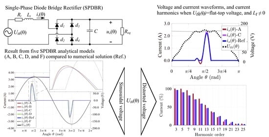
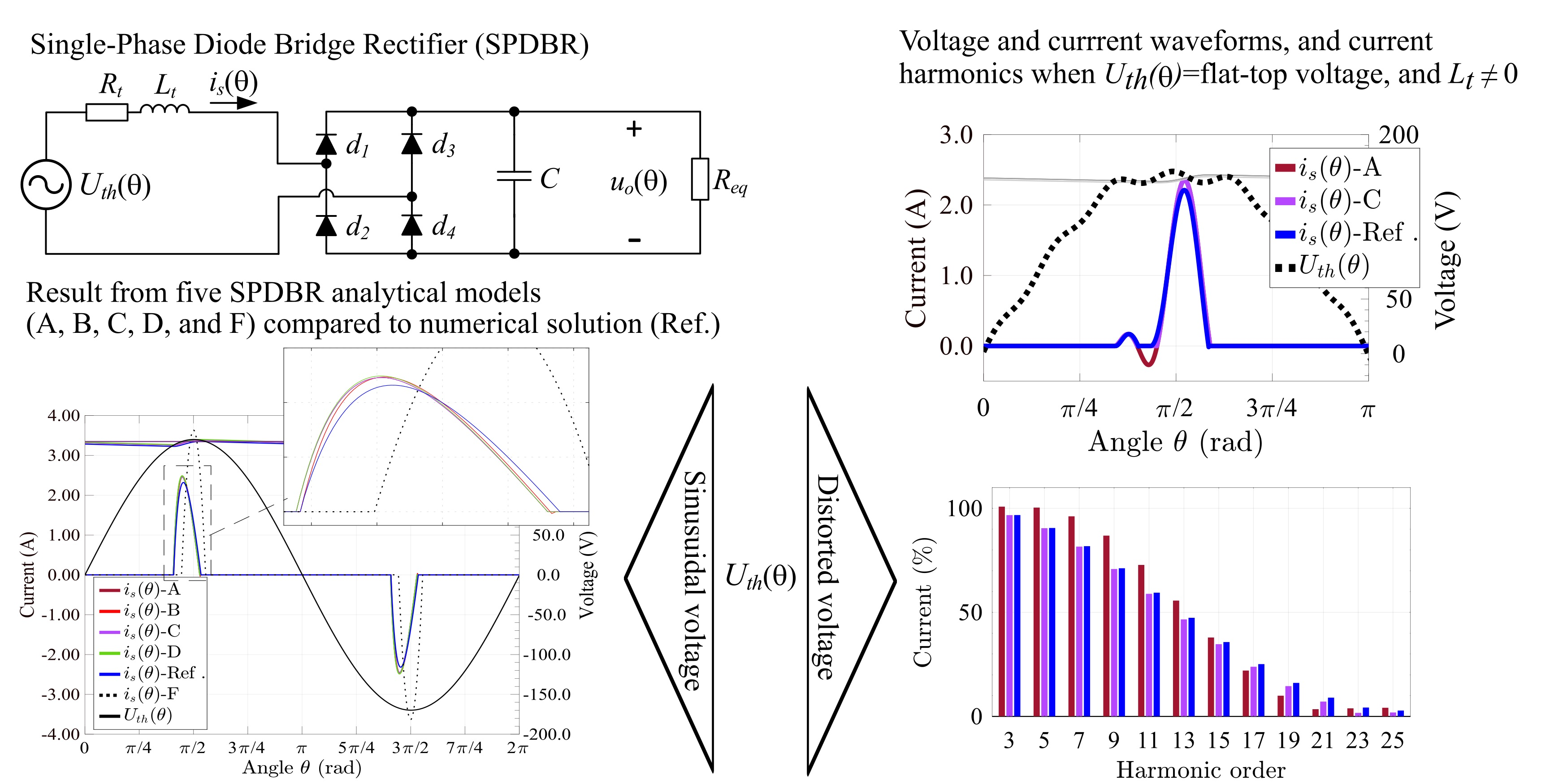
Figure 1a shows a circuit representation commonly used in harmonic studies considering the capacitor-filtered full-bridge diode rectifier connected to the power system.
When the magnitude of the instantaneous supply voltage
exceeds the instantaneous capacitor voltage, the diodes
and
(or
and
) will conduct and charge the capacitor, characterizing the charging period (
Figure 1b), and the equations in this case are:
When the current through the diodes becomes zero, the diodes stop conducting and the capacitor
C will discharge through the load resistance
, as represented in
Figure 1c. In this case, the instantaneous output voltage
can be found by:
Equations (
1) and (
2) work in conjunction with the definition of the instants when the conduction starts and stops. In this regard, different methods give different solutions.
Based on this basic representation, six analytical models of single-phase full-wave bridge rectifiers, summarized in
Table 1, varying in terms of application and complexity, are analyzed in this study.
The models are described by algebraic equations to estimate the input current considering the sinusoidal supply voltage, switching behavior of ideal diodes, and capacitor charging/discharging modes as a function of the equivalent resistance load. Some models consider also the voltage source distortion, impedance of the power system, diode non-ideality, and the ability to include discontinuous conduction mode, i.e., when the input current is characterized by multiple pulses during one half-cycle. From a practical point of view, all models have applicability depending on the required accuracy and level of complexity. However, only models A and C can estimate the input current under voltage source distortion and source impedance with some reactance. Model B also considers source reactance, but neglects the voltage distortion, while models D, E, and F are simpler as they assume ideality in both source impedance and voltage.
2.1. Mansoor’s Model (Model A)
This model is described in [
5] and is an extension of a previous version considering a sinusoidal voltage source [
1]. Based on the circuit shown in
Figure 1, the two differential equations defined in (
1) are solved by the Laplace transform, where
is given by:
The starting and stopping angles for the conduction period,
and
, are determined from two boundary conditions in steady state by using an iterative numerical approach. The model gives the analytical expression for calculating the input current in the time domain:
where the description of the constants
,
to
, and
and
are included in
Appendix A.
2.2. Arrilaga’s Model (Model E)
The model described in [
26] is simpler than the previous model. The harmonics of the current pulse are estimated by using the following Fourier series expression:
where
I is the impulse peak value and
its duration as a proportion of the fundamental cycle period
T. The expressions to obtain
I and
are not given and must be prior assumed, or alternatively estimated through measurements or numerical simulations. Although these requirements make it difficult to compare with other methods presented in this article, the method is still worthwhile in harmonic studies, due to its simplicity, when these two characteristics are well known.
2.3. Mohan’s Model (Model B)
Presented in [
12], Mohan et al.’s model is developed from similar differential equations as in (
1). A noticeable difference from Mansoor’s model (A) is that Mohan’s model (B) uses a trapezoidal rule of integration to solve the differential equations. The starting and stopping conducting angles,
and
, are obtained by an iterative process using the same boundary conditions as in Mansoor’s model (A) [
5]. From this, the model gives the analytical expression considering complex source impedance for the input current.
2.4. Discontinuous Conduction Mode Model (Model C)
For sufficiently high voltage distortion at the device terminals, the diodes and (or and ) can conduct for more than one time interval during one half-cycle. This is known as discontinuous conduction mode (DCM).
While Mansoor’s model (A) only considers CCM, Carpinelli et al. [
27] took advantage of Mansoor’s model (A) in considering the distorted voltage waveform and, based on the same equations, an extended model including the DCM was developed. Carpinelli’s model (C) considers the CCM as a particular case of the DCM and presents a numerical method based on an iterative procedure to obtain the starting and stopping angles for each conduction period.
2.5. Constant DC Voltage Model (Model F)
Assuming, among others, a pure resistive
R source and constant DC output voltage, Bollen and Gu [
13] obtained a simplified model. The idealization lies in the assumption that the AC voltage is sinusoidal (i.e.,
) and that the current at the AC side changes direction instantaneously. Although the DC voltage is not fully constant, in reality, because of its dependency on the DC load, as well as on the AC voltage and source impedance, in steady state, it is considered constant and calculated using conservation of charge. The conduction period is calculated by equating the AC and DC voltages, resulting in the following algebraic equation for the input current:
where
and
is the starting conducting angle and the stopping conduction time occurring at instant
(half a cycle minus the start of conduction). The duration of the positive pulse from
through
, which is a fraction of the half-cycle, is obtained as:
2.6. Diode Piecewise Model (Model D)
The study presented in [
30] by J. Guerra-Pulido describes an in-depth analysis of the different mathematical expressions commonly used in filtered half- and full-wave rectifiers. Although the work has an educational purpose, the conclusions are relevant to other applications as well. The algebraic equation for the input current,
, considering a piecewise model appropriate to study the impact of the diode is given by:
where
is a constant to be found from the condition that the diode current has to be zero at the time at which the conduction is initiated.
2.7. Numerical Simulations (Ref)
Besides the aforementioned methods, there are several methods to obtain employing numerical solutions.
Commonly, numerical solutions use an interactive procedure to obtain a solution within pre-defined tolerances. Differences between numerical solutions rely mainly on the way that the circuit is described and how the numerical integration is performed.
In harmonic studies and circuit analysis, programs for performing numerical simulations, such as Electromagnetic Transients Program (EMTP) and SPICE [
34], are commonly used. EMTP uses nodal analysis with the trapezoidal rule integration for solving electromagnetic transients, while SPICE uses gear and/or trapezoidal integration methods. Particularly in SPICE, the algorithms firstly form a set of nodal equations based on Kirchhoff’s Current Law (KCL) for the circuit. The equations are then rearranged in matrix form and a Gaussian elimination is performed to form an upper triangular matrix, which is solved using back substitution. From this, SPICE tries to iteratively solve the matrix for nodal voltages that satisfy KCL by forming an equation of the form
.
Compared to analytical methods, numerical methods require more computational effort. The accuracy is dependent on the proper component description and simulation tolerances. However, its results are still preferred in terms of measurements as a reference because the uncertainty from component values and the measurement process is eliminated.
4. Time-Domain Analysis
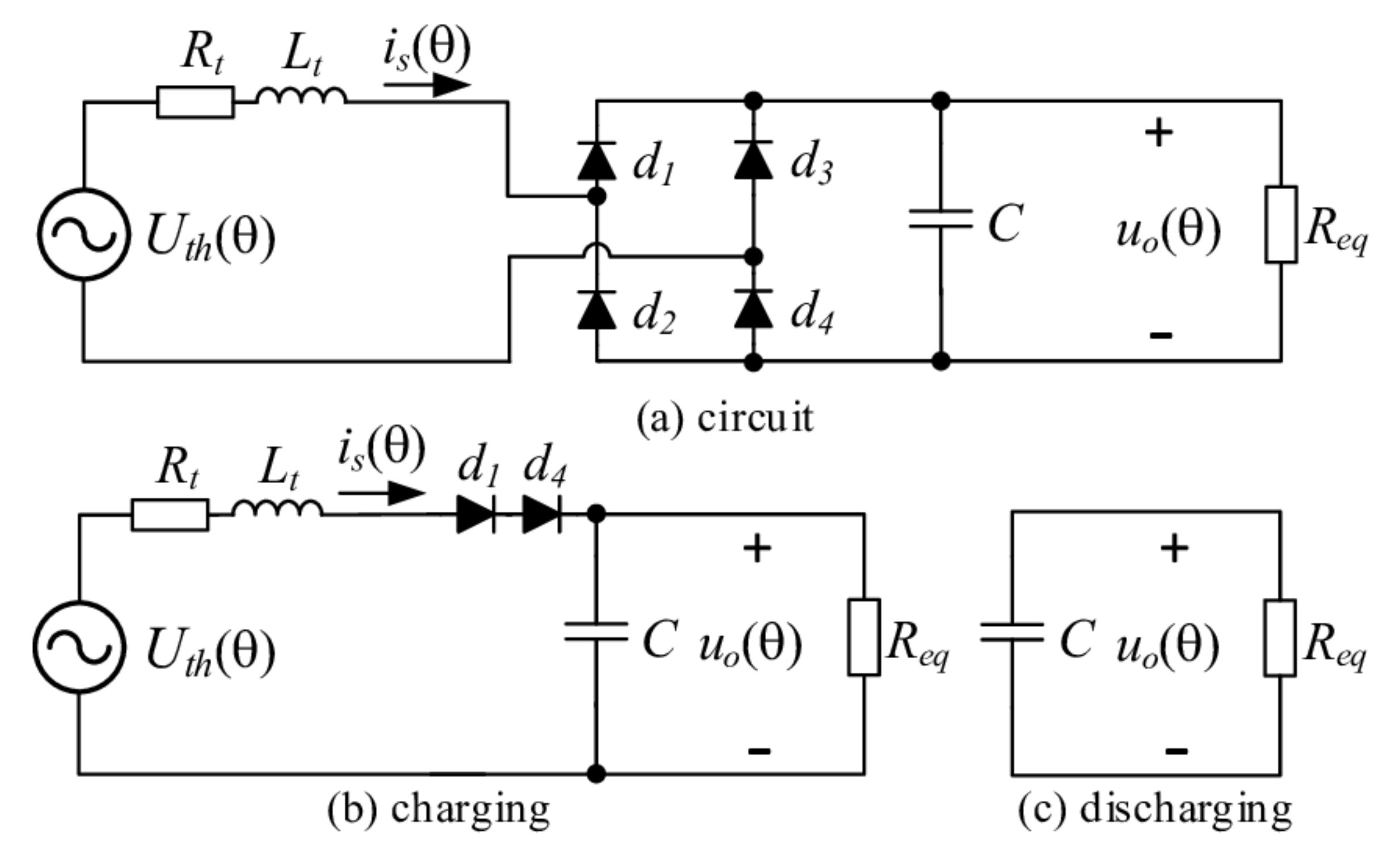
Figure 2 shows the voltage and current waveforms obtained from five different methods for sinusoidal voltage (SI) and resistive source impedance (
). Method E is omitted because of the dependence on prior input data, as discussed in
Section 2. We considered the circuit parameters listed in
Table 2. Results from the models were compared with the numerical solution using PSpice [
37], being identified as Ref. For the simulation, 1N5820 Schottky diodes and the standard simulation parameters of the PSpice software were considered.
From
Figure 2, we observe several differences in the voltage and current waveform, mainly in the starting and stopping phase angles and the maximum value of the current pulse. Taking as a reference the peak current obtained from the numerical solution (blue), which is approximately 2.32 A, the peak current obtained from the analytical models is greater, in the range of 6.06% (i.e., Model B) to 7.35% (i.e., for Model D). One of the hypotheses to explain the difference is that the numerical method has a more precise conduction period, impacting directly on the current peak (i.e., simulation has lower tolerance for solution convergence compared to the analytical model solutions).
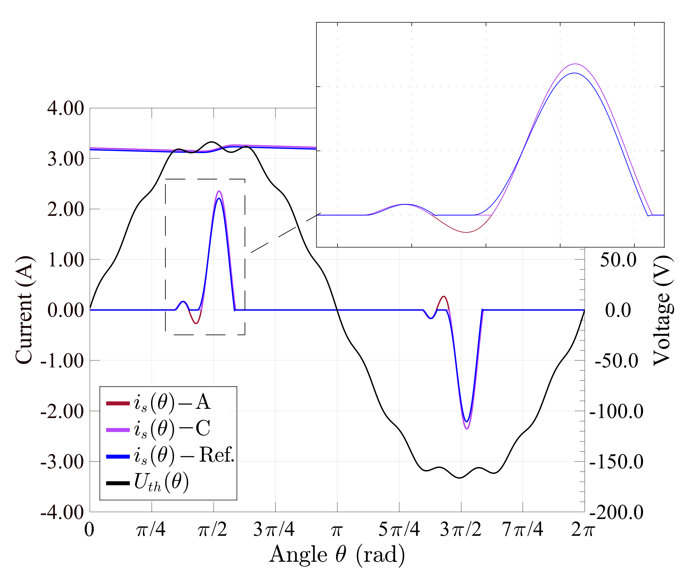
Considering a more realistic scenario with voltage source distortion and inductive source impedance,
Figure 3 shows the current and voltage waveform obtained from models A and C for the flat-top 2 voltage source (
) and inductive network impedance (
). Using the same parameters, the lower graph shows the resulting current and voltage waveforms employing the numerical solution (Ref).
As can be seen in
Figure 3, the current obtained using model A presents an oscillation with reverse conduction, which is unrealistic. The current obtained using model C properly results in discontinuous conduction, confirmed by the numerical solution. Note that model C is similar to model A for the conduction periods because model C uses the same analytical expression during each of the two states.
In order to compare the different models,
Table 5 lists some time-domain indices for current and voltage for different system impedances.
For all the assessed network impedances, there are differences in the maximum current value and conduction angles. In general, the numerical solution presents a lower peak current compared to the results from the analytical models. This happens because the conduction time given by the
from the numerical solution is larger than the
from the analytical models. This occurs because the input current continues after the input voltage reaches its peak. A more detailed explanation for this phenomenon can be found in [
30].
Table 6 lists the results for the distorted voltage source. Because the flat-top and pointed-top waveforms are not able to create any discontinuity in the current, the results from models A and C are the same. However, the flat-top waveform
results in discontinuous conduction, as can be seen by the presence of two conduction periods. The main differences in the resulting values occur for the DC output voltage and conduction angles.
5. Frequency-Domain Analysis
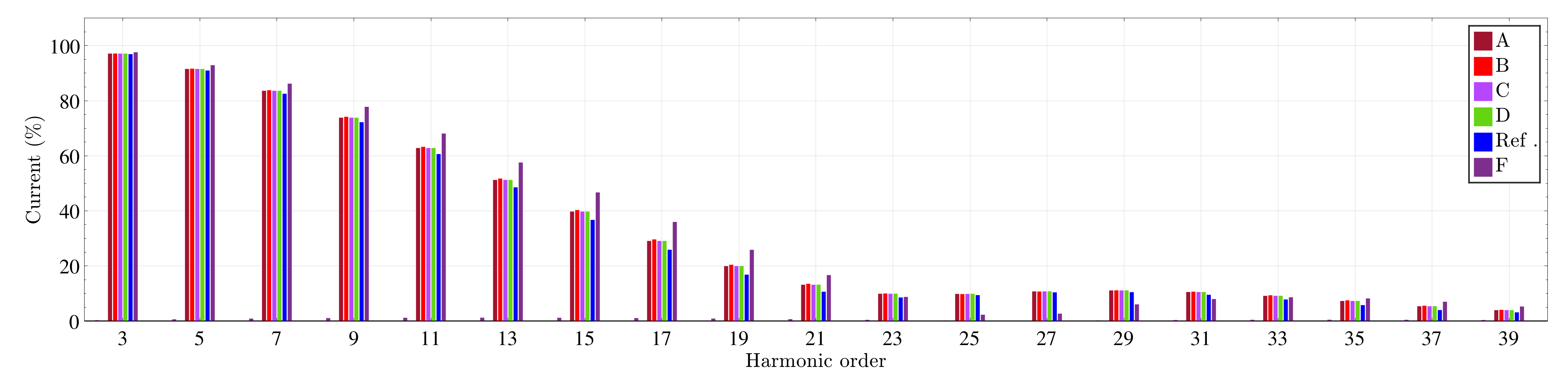
Figure 4 shows the current harmonics obtained from the different models considering a pure sinusoidal voltage source (SI) and system equivalent impedance
. Values are given as percentages, using the fundamental current harmonic component as a reference.
Most of the models have good accuracy and the results are slightly above the reference for the entire harmonic range.
The maximum THD error given by models A, B, C, and D is 2.74%, while the individual harmonic error increases with the harmonic order. For instance, for the harmonics up to the 13th order, the error is less than 6.58% but it can be more than 25% for the harmonics above the 35th order.
Model F (constant DC model) presents the highest error, especially for the higher harmonic orders. The harmonic current tends to remain above the reference up to the 21st harmonic order. After this order, the harmonics become lower than the reference. For instance, for the third harmonic order, the error is only 0.70% but it increases to 18.55% for the 13th order.
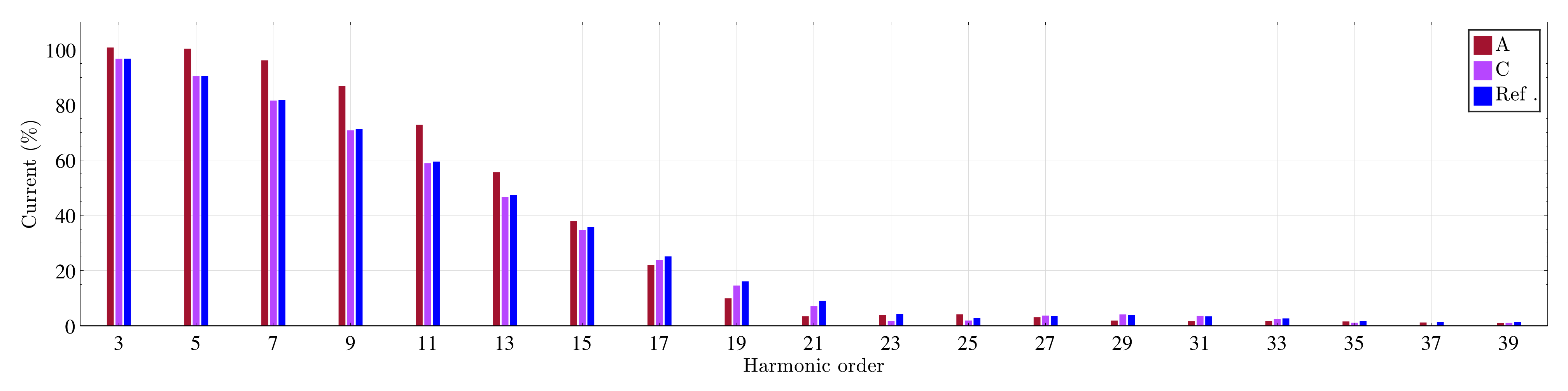
When the impact of voltage source distortion matters, Carpinelli’s model (C) is more accurate than Mansoor’s model (A), as can be seen in
Figure 5.
For the whole harmonic range, model C gives a small THD error compared to the reference. The THD error from model C is only 0.65% while model D gives an error equal to 12.67%. The error for individual harmonics obtained from model C is less than 2.82% for the harmonics below the 15th order, while, in the same range, model A results in an error above 22%.
7. Discussion
7.1. Applicability of the Models
This study shows that most of the analytical models present reasonable accuracy in characterizing the input current in steady state compared to the numerical solution. None of the models show results that are completely wrong under moderate background voltage distortion, but all models have some limitations in their applicability.
The constant DC voltage model (F) has the largest error. However, despite its simplicity, it is the only one without the need for a numerical solution. This enables the fastest solution while still maintaining accuracy that may be sufficient for some applications. For large stochastic studies (e.g., considering a few dozen consumers with multiple and distinct single-phase bridge rectifiers), this may be the only possible model for a fast estimation of the harmonic distortion.
For medium-sized stochastic studies, models A, B, C, and D may be possible as well. The results for these four models are very similar, as shown in
Figure 4. The deviation from the reference model is roughly the same for all of them. The additional complexity introduced in some of the models does not pay off for studies of moderate complexity. In this context, the choice should be based on whether to consider background voltage distortion and DCM. If these two factors are not relevant, model B gives the simplest solution.
All models consider the impact of voltage distortion due to the device itself or due to similar devices nearby, but only some of the models (i.e., A and C) consider the impact of voltage distortion due to external sources (“background voltage distortion”). As shown in
Figure 5, this is where the results from model C are closer to the reference model (Ref) than the results from model A. The difference is relatively large. When including the background voltage distortion, rather accurate results are usually desired. This means that stochastic studies or detailed studies with many components are still not possible.
Regarding the system scale, the iterative numerical approach needed by most of the analytical models will create additional complexity for the power-flow solution convergence. In this respect, simple models such as model F have significant advantages as the performance is less dependent on the power flow solution. In a power system, the analytical models employing iterative numerical approaches, such as models A, B, C, and D, will have different behavior compared to the individual performance. The computation times given in
Table 7 are only valid as a reference under a steady-state condition. There are aggregation issues, and the system might not converge under several analytical models.
7.2. Analytical Model versus Numerical Solution
Numerical methods are still the best choice where accuracy is concerned. However, even considering the simple circuit of a single-phase bridge rectifier, computing effort is a serious limitation, especially if the system contains multiple devices. Considering background voltage distortion in general further increases the difficulty for the iterative process to reach convergence.
Models based on analytical expressions are often much faster to give results compared to numerical methods. Additionally, these models immediately give the stationary solution, which is desirable in harmonic studies. We can also observe that all the models presented certain differences and limitations compared to numerical solutions. As we increase the elements in the mathematical expressions (e.g., better diode models, background voltage distortion, etc.), the accuracy will improve, but the complexity will increase.
Methods based on analytical expressions are, in most cases, dependent on the solution of transcendental equations, which implies that the solution can only be obtained by a numerical method. However, these methods easily reach convergence and are, in general, faster than a numerical solution considering all the circuit details.
7.3. Discontinuous and Continuous Mode
Carpinelli’s study [
27] mentions that it is rare under normal operation to obtain more than three conduction intervals. The most commonly reported scenario was only one conduction interval and, in some cases, two or three. This conclusion was reached nearly two decades ago, based on a limited set of measurements in the harmonic range. With the fast inclusion of nonlinear loads, this scenario may no longer be representative. Although just one conduction interval (CCM) is the most common scenario, for certain background voltage and system impedance, DCM operation can occur and impact the performance of devices. For instance, the study presented in [
38] showed that DCM occurs at frequencies above 2 kHz, impacting the light intensity of LED lamps.
When a rectified load is subject to a flat-top voltage distortion, it is more likely to create discontinuous conduction because the flat interval remains closer to the DC voltage during a longer period of the cycle. In this particular case, the higher-order harmonics create oscillations in the region where the AC and DC voltage are close. As a result, the current pulse is distorted by the repetitive partial capacitor charging and discharging. The likelihood of DCM further increases if the harmonic phase places the harmonic peak close to the zero-crossing region. Additionally, a dynamic DC load could also create DCM, not only the fact that the voltage source is distorted. For instance, a battery charger changes the equivalent resistance during the charging process. DCM can occur at different stages of the charging process.
In summary, harmonic studies become especially of interest for cases with high distortion, where DCM is more likely to occur. In this respect, model C would be a suitable candidate for stochastic studies, even though it has the most complicated structure among the evaluated models.
7.4. Limitations of the Available Methods
In general, the methods evaluated in this study present differences in the starting and stopping phase angles compared to the reference; this results in small deviations, especially in the time-domain representation. Additionally, most of the methods do not consider background voltage distortion, which is a common reality for most of the applications and can lead to nonlinear interaction [
3]. As shown in
Section 4 and
Section 5, models considering background voltage distortion have better accuracy. Additionally, some models do not consider inductance in the system impedance, which further limits their practical application.
Another limitation is the assumption of the ideal diodes, with the exception of model D. For a high-voltage source level, the constant voltage drop placed by the diodes, , might be neglected, but as the input voltage decreases, the importance of considering a more accurate diode model increases as will impact the current peak and the conducting period.
The internal diode resistance has also great importance, especially in strong grids. Assuming that the total resistance seen by the device will be composed of the network and local system resistance plus the diodes’ internal resistance (i.e., , as two conducting diodes are always placed in series), the relation between resistance matters. For instance, if we consider a system network with , and diodes with (i.e., a common value used in simulation studies), the internal resistance of the diodes will represent one third of the total resistance.
A final remark should be also given to the equivalent DC load. All the models presented in this study assume a resistive load, on the basis of the voltage and current characteristics of the back-end circuits (e.g., DC-to-DC and PFC converters). Although there is a general consensus on this assumption, it is not clear how loads with a parcel of inductive and capacitive characteristics could impact the results.
7.5. Future Work
On the basis of the findings presented in this study, the authors propose that further research should be undertaken in the following areas:
Aggregation of similar but not exactly the same devices, i.e., different diode bridge rectifiers, e.g., with different capacitor sizes.
Similar simplified models for other types of devices, e.g., three-phase rectifiers and Automatic Power Factor Controller (APFC) devices.
Suitable but simplified models for high distortion cases.
Application of the models in stochastic models to compare the stochastic results for simple and accurate models.
Application of the models in harmonic studies considering distribution networks with different characteristics.
Models that consider more detailed DC loads, i.e., including inductive and capacitive characteristics, and nonlinear DC loads.
8. Conclusions
This paper presents a comparison of different analytical models of single-phase diode bridge rectifiers. The models were evaluated and compared with a numerical solution under different background voltage distortion and equivalent system impedance.
Most of the analytical models have accuracy that is sufficient to render them a low-computational alternative to the numerical solution.
The results show that, in general, the analytical models give a reasonable representation of the input current in the time and frequency domain for continuous conduction mode. The highest error is observed at the higher harmonic orders. For high background voltage distortion leading to discontinuous conduction mode, only one model is appropriate. It was also found that all models presented differences and limitations compared to the reference model.
The trade-off involves accuracy and complexity, and there will be applications for all models. From the simplest to the most detailed model, there is applicability to stochastic studies with many components up to studies where the accurate modeling of high-voltage distortion is needed.
Further work is needed towards the application of the models and towards the development of additional models, especially for high distortion cases.


