
Optimal Operation of Multiple Energy System Based on Multi-Objective Theory and Grey Theory


Abstract
:1. Introduction
- (1)
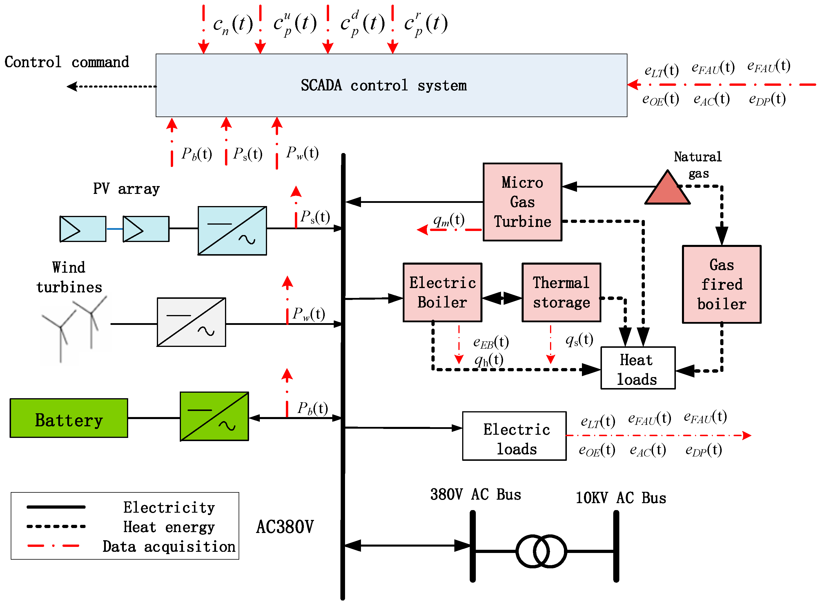
- Combining wind power, photoelectric power, an energy storage system, and a gas system, the energy management system is designed with a focus on the economy and on greenhouse gas emissions.
- (2)
- This paper proposes a grey multi-target linear planning algorithm and optimizes multi-target multi-energy management using the grey multi-target linear planning algorithm.
2. Problem Formulations
2.1. Objective Function
- The energy consumption costs
- 2.
- The waste gas emissions
- 3.
- The components maintenance costs
2.2. Energy Balance Constraints
- The electricity supply and demand constraint
- 2.
- Heating supply constraints
- 3.
- Cooling supply constraints
2.3. Cost of Electricity, Natural Gas and Equipment Maintenance
- Cost of electricity
- 2.
- Cost of natural gas
- 3.
- Cost of equipment maintenance
- 4.
- Cost of electric boiler maintenance
- 5.
- Cost of gas fired boiler maintenance
- 6.
- Cost of micro gas turbine maintenance
- 7.
- Cost of thermal storage maintenance
2.4. Constraints of Equipment Electricity and Heat Output
- Constraint of heat output of the electric boiler
- 2.
- Constraint of heat output of the thermal storage
- 3.
- Constraint of heat output of the gas fired boiler
- 4.
- Constraint of electricity output of the battery
- 5.
- Constraint of output of the micro gas turbine
3. Solution Methodology
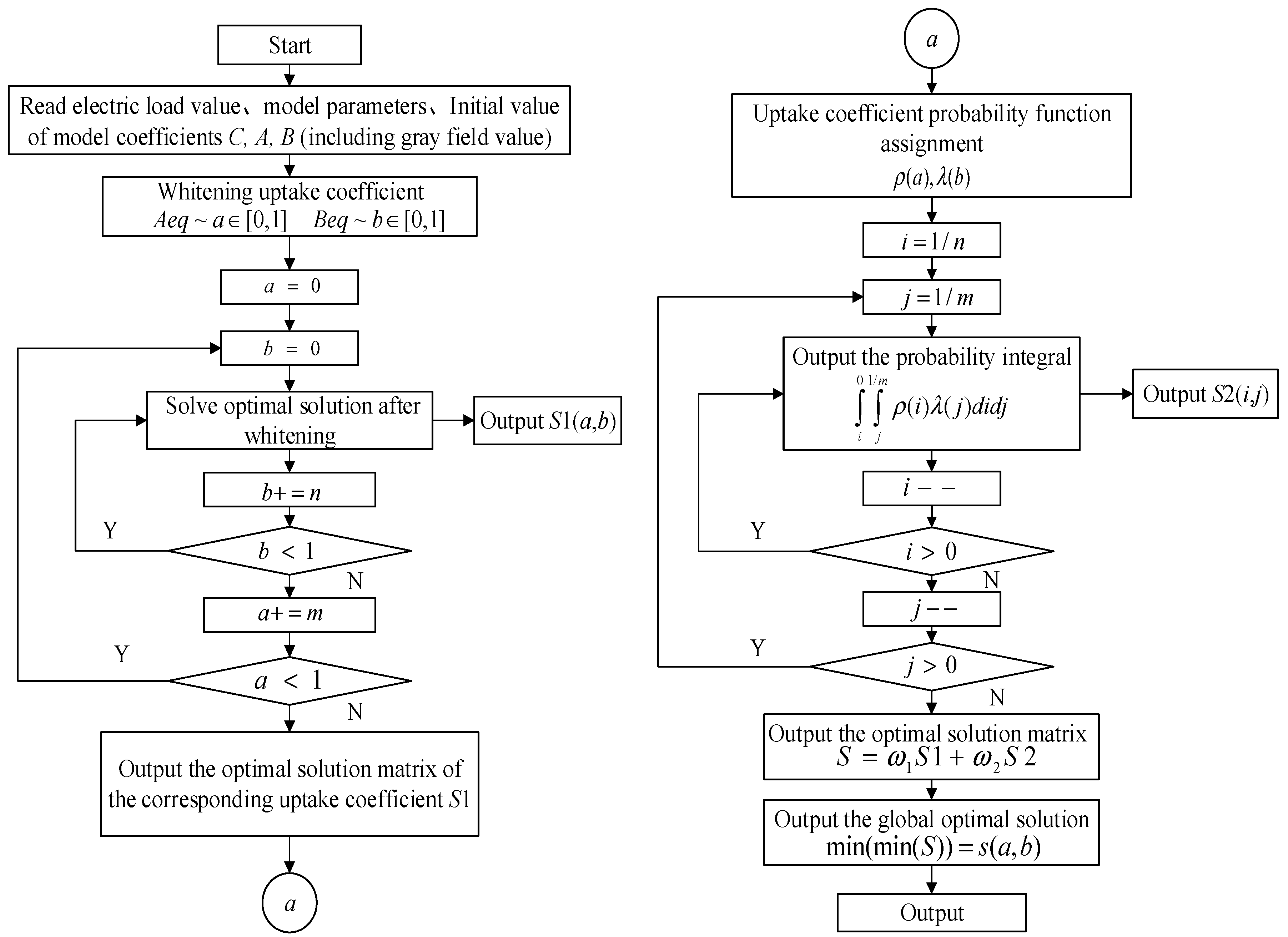
3.1. Grey Multi-Objective Linear Programming Algorithm
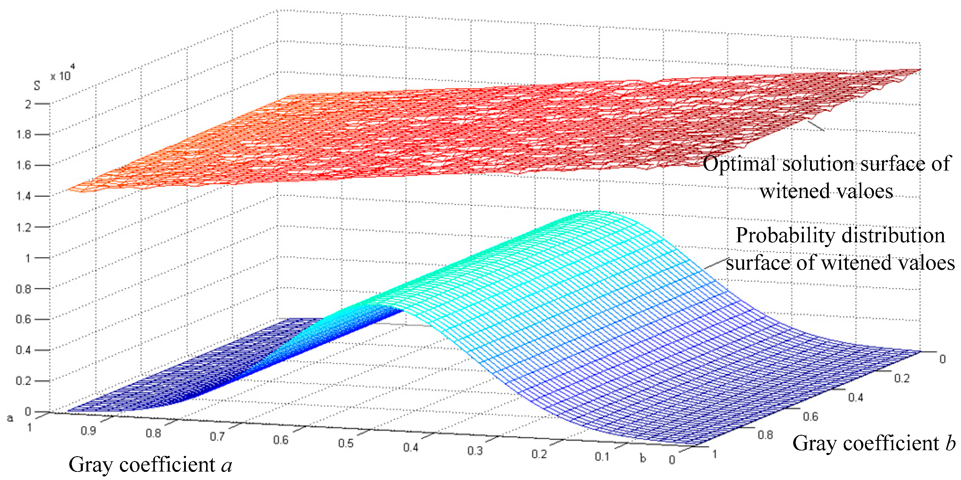
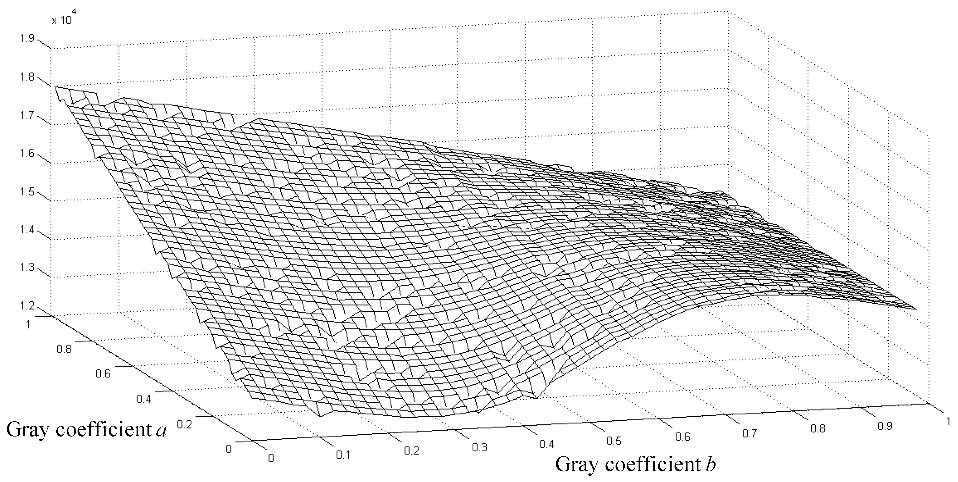
3.2. Model Solving Method
4. Numerical Results
4.1. Example Analysis

| Time (h) | ||||||||
|---|---|---|---|---|---|---|---|---|
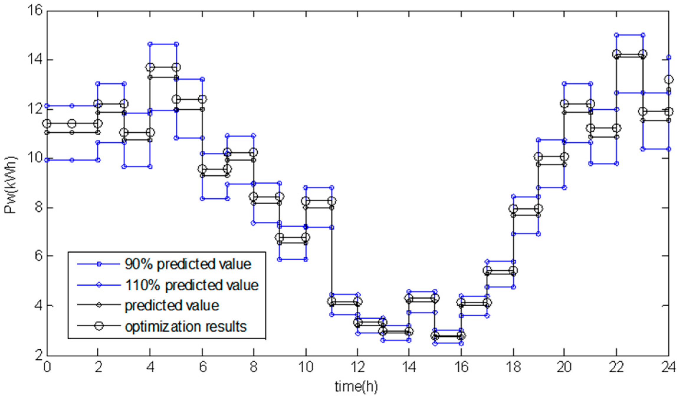
| 21 | 9.792 | 11.968 | 0.00 | 0.00 | 1.3 | 1.6 | 14.9 | 18.2 |
| 22 | 12.672 | 15 | 0.00 | 0.00 | 2.5 | 3.1 | 14.9 | 18.2 |
| 23 | 10.368 | 12.672 | 0.00 | 0.00 | 2.5 | 3.1 | 14.9 | 18.2 |
| 24 | 11.52 | 14.08 | 0.00 | 0.00 | 2.1 | 2.5 | 14.5 | 17.7 |
| 1 | 9.936 | 12.144 | 0.00 | 0.00 | 1.3 | 1.6 | 14.9 | 18.2 |
| 2 | 10.656 | 13.024 | 0.00 | 0.00 | 1.3 | 1.6 | 14.9 | 18.2 |
| 3 | 9.648 | 11.792 | 0.00 | 0.00 | 1.3 | 1.6 | 14.9 | 18.2 |
| 4 | 11.952 | 14.608 | 0.00 | 0.00 | 1.3 | 1.6 | 14.9 | 18.2 |
| 5 | 10.8 | 13.2 | 0.00 | 0.00 | 1.3 | 1.6 | 14.9 | 18.2 |
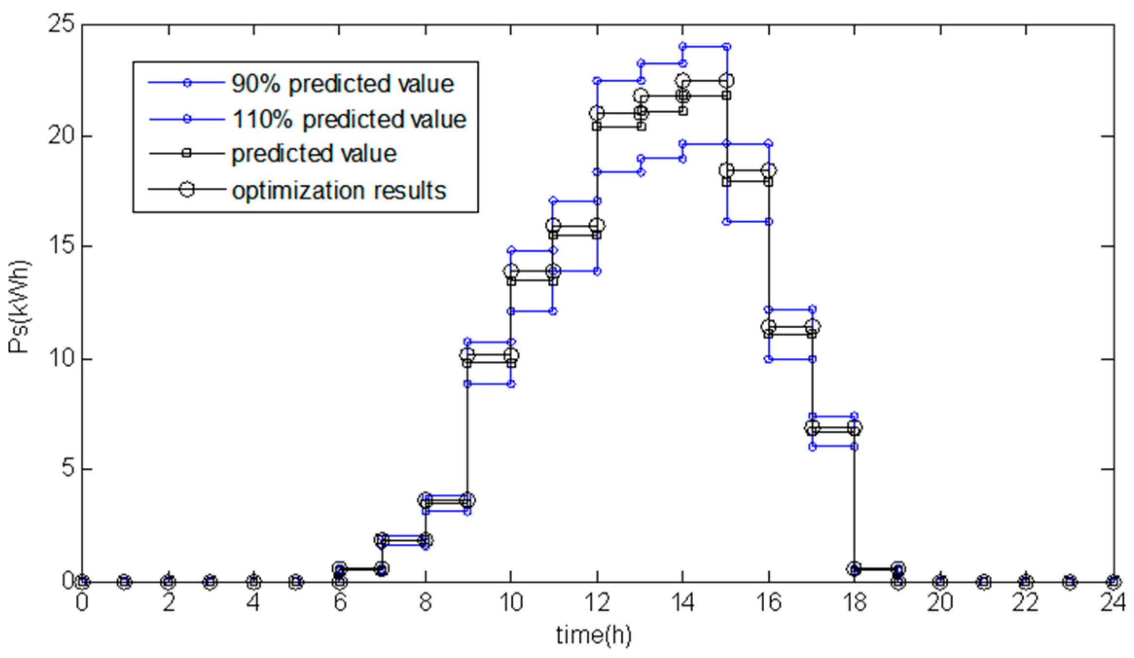
| 6 | 8.352 | 10.208 | 0.45 | 0.55 | 2.5 | 3.1 | 14.9 | 18.2 |
| 7 | 8.928 | 10.912 | 1.62 | 1.98 | 1.3 | 1.6 | 14.9 | 18.2 |
| 8 | 7.344 | 8.976 | 3.15 | 3.85 | 1.3 | 1.6 | 39.3 | 48 |
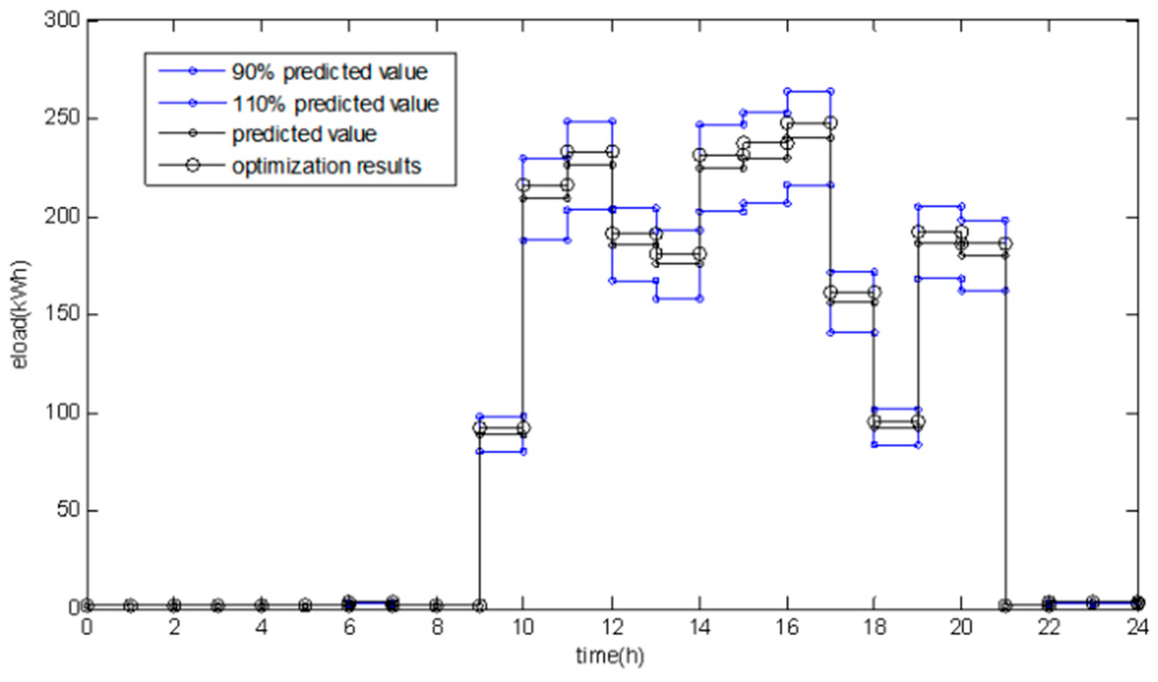
| 9 | 5.904 | 7.216 | 8.82 | 10.78 | 79.8 | 97.5 | 39.7 | 48.5 |
| 10 | 7.2 | 8.8 | 12.15 | 14.85 | 188.0 | 229.8 | 36.9 | 45.1 |
| 11 | 3.6288 | 4.4352 | 13.95 | 17.05 | 203.2 | 248.3 | 51.7 | 63.2 |
| 12 | 2.88 | 3.52 | 18.36 | 22.44 | 166.9 | 204.0 | 75.2 | 92 |
| 13 | 2.592 | 3.168 | 18.99 | 23.21 | 157.7 | 192.8 | 63.2 | 77.2 |
| 14 | 3.744 | 4.576 | 19.62 | 23.98 | 201.9 | 246.8 | 57.1 | 69.8 |
| 15 | 2.448 | 2.992 | 16.11 | 19.69 | 206.6 | 252.6 | 70.8 | 86.6 |
| 16 | 3.6 | 4.4 | 9.99 | 12.21 | 216.0 | 264.0 | 47.2 | 57.7 |
| 17 | 4.752 | 5.808 | 6.03 | 7.37 | 140.4 | 171.5 | 52.9 | 64.6 |
| 18 | 6.912 | 8.448 | 0.45 | 0.55 | 83.0 | 101.4 | 38 | 46.5 |
| 19 | 8.784 | 10.736 | 0.00 | 0.00 | 167.6 | 204.8 | 28.6 | 34.9 |
| 20 | 10.656 | 13.024 | 0.00 | 0.00 | 161.9 | 197.8 | 16.1 | 19.6 |
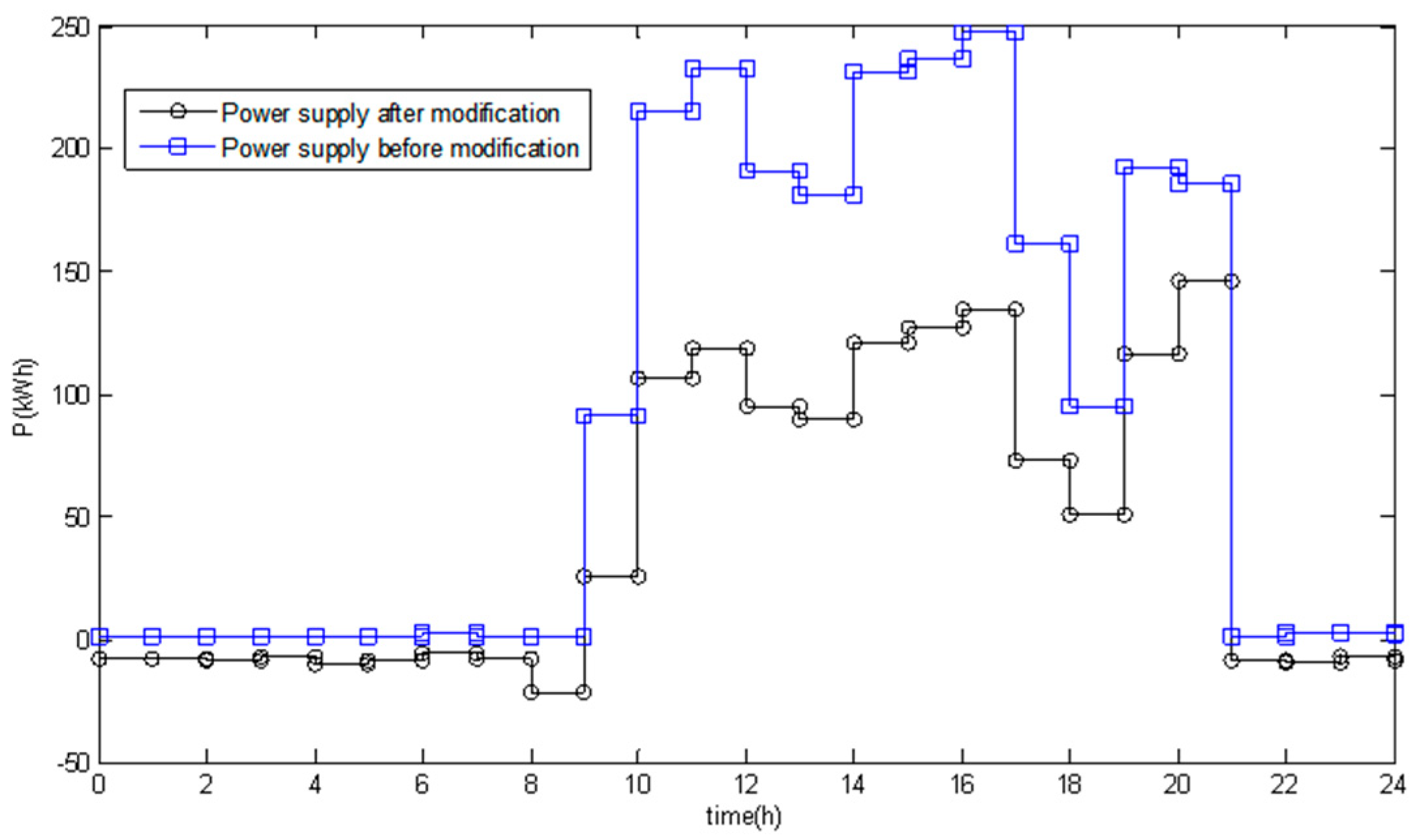
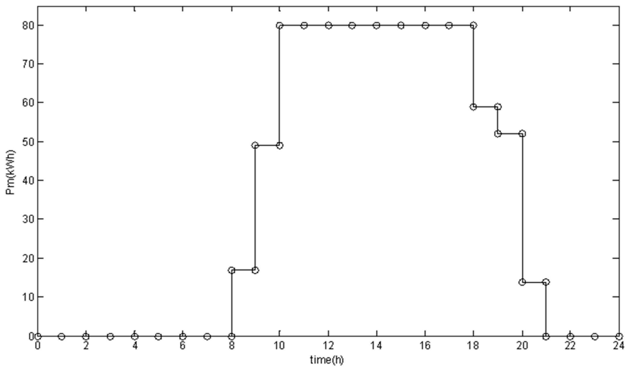
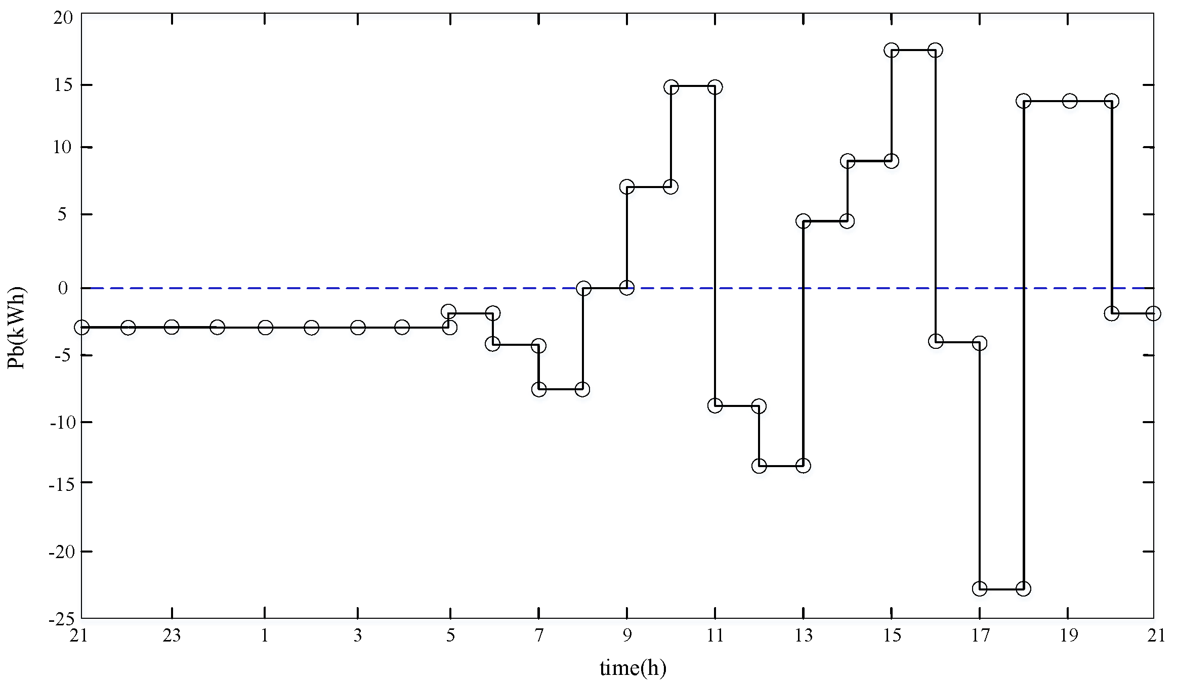
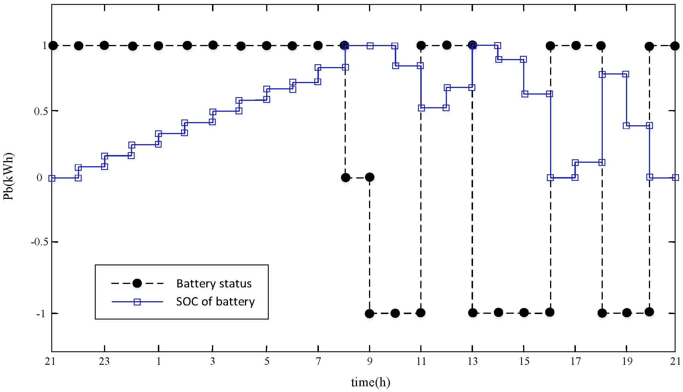
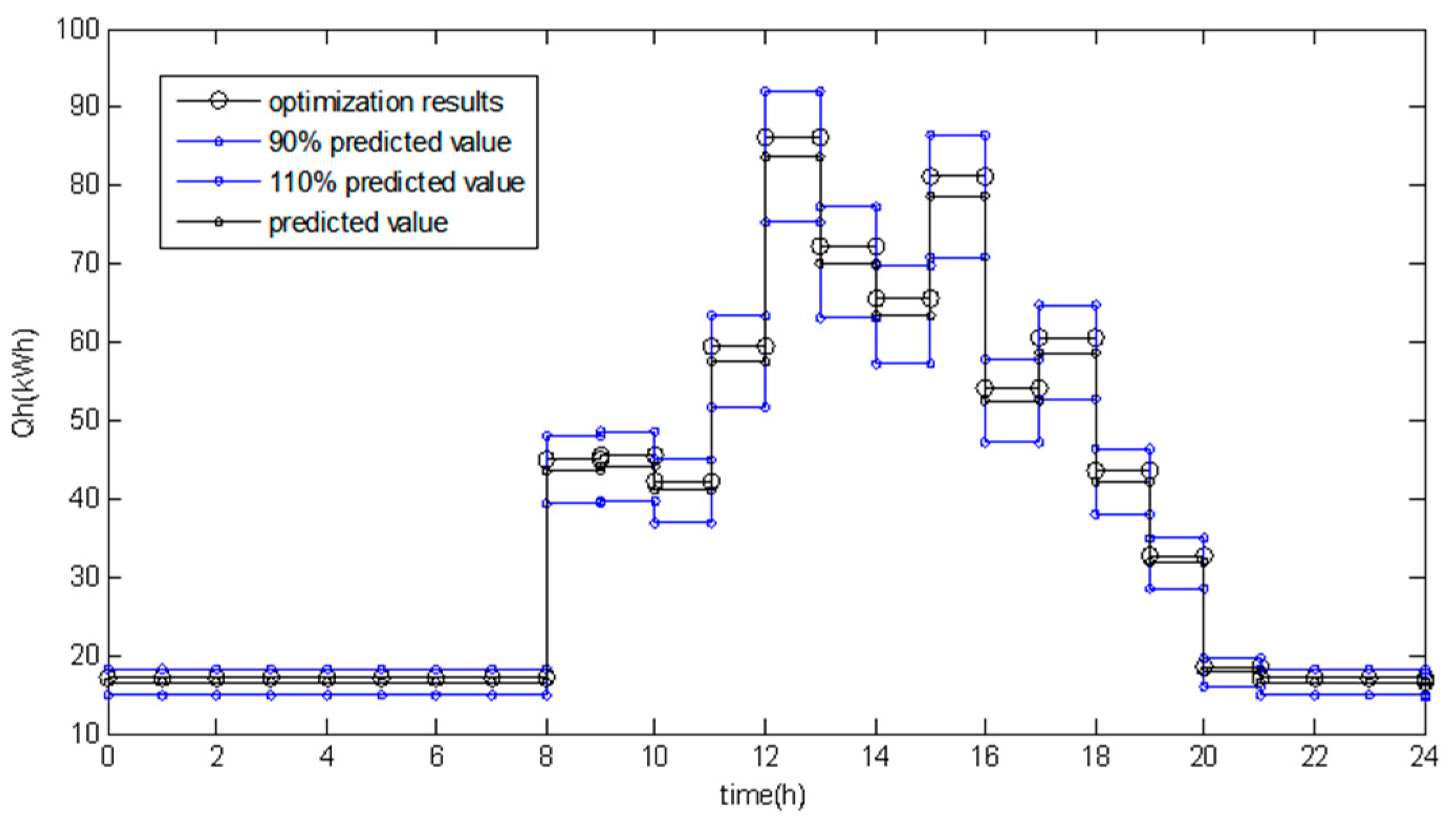
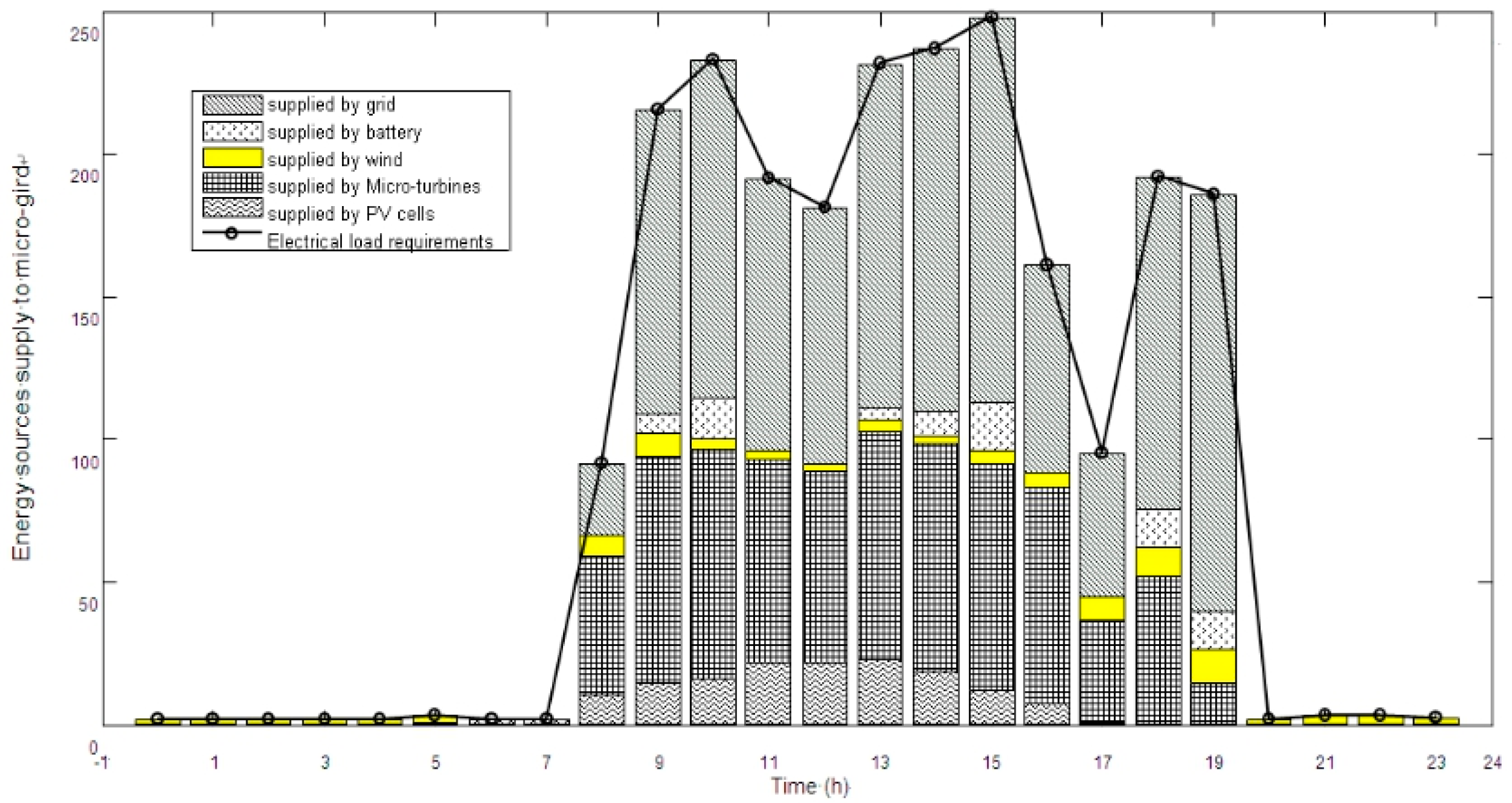
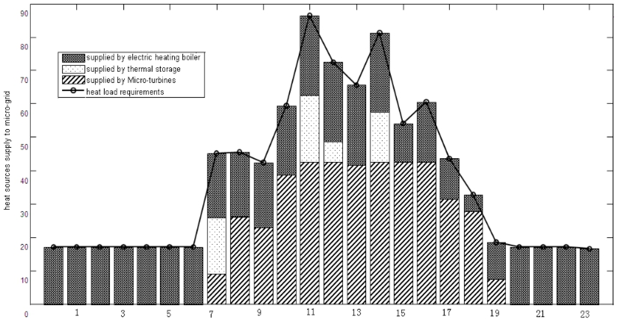
4.2. Simulation Result
5. Conclusions
- (1)
- Combining wind power, photoelectric power, an energy storage system, and a gas system, the energy management system is designed focused on the economy and on greenhouse gas emissions. Considering the actual operation of a multi-energy microgrid system, in order to make the energy management scheme more practical, a variety of optimization objectives and constraints are proposed in this paper. The optimization objectives and constraints are determined not only by taking into account the economic cost of micro-network operations, but also by mathematically modeling the exhaust emissions when the system is run and by setting the corresponding energy control targets in terms of economic benefits and environmental protection.
- (2)
- For the possible uncertainty resulting when constructing the multi-objective model and the constraints in practical engineering cases, the grey multi-objective linear planning algorithm is proposed. Using the grey multi-target linear planning algorithm, the multi-target multi-energy optimization management of a microgrid is realized. By comparisons with multiple optimization methods, the economic costs of the proposed method are verified and the amount of cost savings and the cost recovered using our method are analyzed. The verification results meet the optimized operating conditions of a multi-energy microgrid system after analysis.
Author Contributions
Funding
Institutional Review Board Statement
Informed Consent Statement
Data Availability Statement
Conflicts of Interest
Nomenclature
| Total cost of electricity during t (USD). | |
| Total cost of natural gas during t (USD). | |
| Power from the grid during t (kw) | |
| Clean power generation during t (kWh) | |
| Natural gas consumption during t (m3) | |
| Buying price of electricity during t (USD/kWh) | |
| Selling price of electricity during t (USD/kWh). | |
| Spontaneous self-used subsidy electricity price of electricity during t (USD/kWh). | |
| Natural gas price of electricity during t (USD/kWh) | |
| Time interval | |
| Exhaust gas amount produced by using electricity during t | |
| Exhaust SOX amount produced by using electricity during t | |
| Exhaust NOX amount produced by using electricity during t | |
| Exhaust CO2 amount produced by using electricity during t | |
| Exhaust SOX amount produced by using gas turbines during t | |
| Exhaust NOX amount produced by using gas turbines during t | |
| Exhaust CO2 amount produced by using gas turbines during t | |
| Exhaust SOX amount produced by using gas fired boiler during t | |
| Exhaust NOX amount produced by using gas fired boiler during t | |
| Exhaust CO2 amount produced by using gas fired boiler during t | |
| Maintenance cost of the battery (USD) | |
| Maintenance cost of the photovoltaic cells (USD) | |
| Maintenance cost of the wind turbines (USD) | |
| Maintenance cost of the electric boiler (USD) | |
| Maintenance cost of the micro gas turbines (USD) | |
| Maintenance cost of the micro gas fired boiler (USD) | |
| Maintenance cost of the heat accumulator (USD) | |
| Total electricity load demand during t (kWh) | |
| Electricity provided by the photovoltaic cells during t (kWh) | |
| Electricity provided by the wind turbines during t (kWh) | |
| Electricity provided by the micro gas turbines during t (kWh) | |
| Electricity provided by the battery during t (kWh), charge (>0) or discharge (<0) | |
| Total heat demand during t (kWh). | |
| Heat provided by the electric boiler during t (kWh) | |
| Heat provided by the gas fired boiler during t (kWh) | |
| Heat provided by the heat accumulator during t (kWh) | |
| Heat provided by the micro gas turbines during t (kWh) | |
| Heat converse rate of the heat accumulator during t | |
| Heat converse rate of the micro gas turbines during t | |
| Heat converse rate of the electric boiler during t | |
| Heat converse rate of the electric boiler during t | |
| Discrete variable, “1” for the battery charging during t, “0,” otherwise. | |
| Discrete variable, “1” for the battery discharging during t, “0,” otherwise. | |
| Discrete variable, “1” for the micro gas turbines running during t, “0,” otherwise. | |
| Discrete variable, “1” for the heat accumulator charging during t, “0,” otherwise. | |
| Discrete variable, “1” for the heat accumulator discharging during t, “0,” otherwise. | |
| Discrete variable, “1” for the electric boiler running during t, “0,” otherwise. | |
| Discrete variable, “1” for the gas fired boiler running during t, “0,” otherwise. | |
| Discrete variable, “1” for the micro gas turbines running during t, “0,” otherwise. | |
| Gas consumption of gas fired boiler | |
| Rated power of the electric boiler (kW) | |
| Rated power of the gas fired boiler (kW) | |
| Rated power of the heat accumulator (kW) | |
| Remaining heat energy in the heat accumulator device during t(kWh). | |
| Heat energy supplied by the heat accumulator device during t(kWh). | |
| Minimal heat load rate of the heat accumulator (kW) | |
| Maximal heat load rate of the heat accumulator (kW) | |
| Minimal discharge rate of the battery (kW) | |
| Maximal discharge rate of the battery (kW) | |
| Electrical load ratio of the micro gas turbines during t, | |
| Capacity of the micro gas turbines (kWh) |
References
- Teng, Y.; Sun, P. Operation optimization model of micro-energy grid considering biomass waste classification and treatment. Autom. Electr. Power Syst. 2021, 45, 55–63. [Google Scholar]
- Zhi, N.; Xiao, X.; Tian, P.G. Research status and prospect of microgrid group control technology. Electr. Power Autom. Equip. 2016, 36, 107–115. [Google Scholar]
- Fan, Z.; Fan, B.; Peng, J.K. Operation Loss Minimization Targeted Distributed Optimal Control of DC Microgrids. IEEE Syst. J. 2020, 15, 5186–5196. [Google Scholar] [CrossRef]
- Sang, B.; Zhang, T.; Liu, Y.J. Review on energy management system of multi-micro grid. Proc. CSEE 2020, 40, 3077–3093. [Google Scholar]
- Yin, L.J.; Zhao, X.L.; Mei, Z. Optimizing Technology for Micro Grid Operation Based on Chaos Particle Swarm Optimization Algorithm. Proc. CSU-EPSA 2016, 28, 55–61. [Google Scholar]
- Chen, J.; Liu, Y.T.; Zhang, W. Analysis of optimal configuration of multistage microgrid in distribution network based on game theory. Proc. CSU-EPSA 2016, 40, 45–52. [Google Scholar]
- Rokicki, Ł. Optimization of the Configuration and Operating States of Hybrid AC/DC Low Voltage Microgrid Using a Clonal Selection Algorithm with a Modified Hypermutation Operator. Energies 2021, 14, 6351. [Google Scholar] [CrossRef]
- Riou, M.; Dupriez-Robin, F.; Grondin, D. Multi-Objective Optimization of Autonomous Microgrids with Reliability Consideration. Energies 2021, 14, 4466. [Google Scholar] [CrossRef]
- Hu, C.; Luo, S.; Li, Z. Energy Coordinative Optimization of Wind-Storage-Load Microgrids Based on Short-Term Prediction. Energies 2015, 8, 1505–1528. [Google Scholar] [CrossRef] [Green Version]
- Fatrias, D.; Alfadhlani; Kamil, I. Using grey-fuzzy programming approach to solve multi-objective supplier selection problem. In Proceedings of the 2017 4th International Conference on Industrial Engineering and Applications (ICIEA), Nagoya, Japan, 21–23 April 2017; Volume 4, pp. 141–145. [Google Scholar]
- Wang, W.; Li, R.; Jiang, J.C. Key Issues and Research Prospects of Distribution System Planning Orienting to Energy Internet. High Volt. Eng. 2016, 42, 2028–2036. [Google Scholar]
- Li, L.; Luo, Z.; He, F.; Sun, K.; Yan, X. An improved partial similitude method for dynamic characteristic of rotor systems based on Levenberg–Marquardt method. Mech. Syst. Signal Processing 2022, 165, 108405. [Google Scholar] [CrossRef]
- He, L.J.; Li, W.F.; Zhang, Y. Application of Gray Relational Analysis in Optimization of Automotive Panel Forming. Control Decis. 2020, 35, 1134–1142. [Google Scholar]
- Hu, Z.B.; Li, Z.; Dai, C.Y. Multiobjective Grey Prediction Evolution Algorithm for Environmental/Economic Dispatch Problem. IEEE Access 2020, 8, 84162–84176. [Google Scholar] [CrossRef]
- Zhao, H.; Guo, S.; Zhao, H. Selecting the Optimal Micro-Grid Planning Program Using a Novel Multi-Criteria Decision Making Model Based on Grey Cumulative Prospect Theory. Energies 2018, 11, 1840. [Google Scholar] [CrossRef] [Green Version]
- He, X.H.; Yang, J.Y. Grey PSO algorithm-based multi-objective optimization of Scheduling of distributed power grid with peak load regulation. Journal of Lanzhou University of Technology. IEEE Trans. 2018, 44, 79–83. [Google Scholar]
- Xiong, Y.F.; Chen, L.J.; Zheng, T.W. Optimal configuration of hydrogen energy storage in comprehensive energy system of low-carbon industrial park considering the coupling characteristics of electricity and heat. Electr. Power Autom. Equip. 2021, 41, 31–38. [Google Scholar]
- Chen, J.P.; Hu, Z.J.; Chen, Y.G. Thermoelectric optimization of integrated energy system considering stepped carbon trading mechanism and electric hydrogen production. Electr. Power Autom. Equip. 2021, 41, 48–55. [Google Scholar]
- Jiao, S.M.; Qiao, X.B.; Li, Y. Combined optimization of power-to-gas equipment and photovoltaic, taking into account the life-cycle carbon emissions and carbon trading of the integrated energy system. Electr. Power Autom. Equip. 2021, 41, 156–163. [Google Scholar]
- Haider, Z.M.; Mehmood, K.K.; Khan, S.U.; Khan, M.O.; Wadood, A.; Rhee, S.-B. Optimal Management of a Distribution Feeder during Contingency and Overload Conditions by Harnessing the Flexibility of Smart Loads. IEEE Access 2021, 9, 40124–40139. [Google Scholar] [CrossRef]


| Time (h) | - | 5:00–7:00 | - |
| 7:00–12:00 | 12:00–17:00 | - | |
| 17:00–21:00 | 21:00–22:00 | 22:00–5:00 | |
| Price (RMB/kWh) | 0.7482 | 0.4988 | 0.2494 |
| Power Type | Pollution Coefficient (g/kWh) | Equipment Capacity (kW) |
|---|---|---|
| Power grid | 889 | - |
| Wind turbines | 0 | 15 |
| PV cells | 0 | 28 |
| Micro gas turbine | 724.6 | 80 |
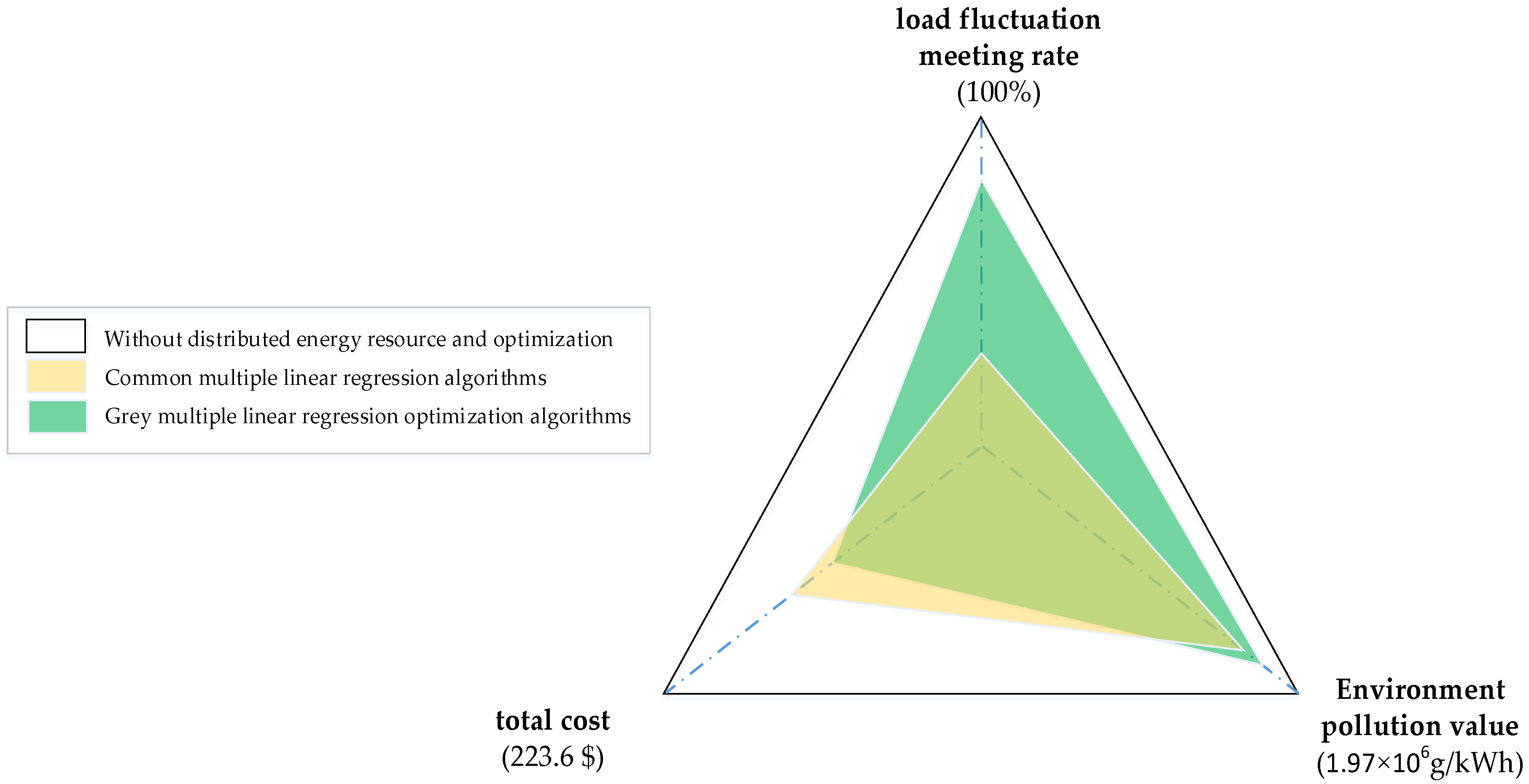
| Optimization Method | load Fluctuation Meeting Rate | Total Cost ($) | Environment Pollution Value (g/kWh) |
|---|---|---|---|
| Without distributed energy resource and optimization | 100% | 223.6 | 1.97 × 10⁶ |
| Common multiple linear regression algorithms | 25% | 187.3 | 1.6 × 10⁶ |
| Grey multiple linear regression optimization algorithms | 87% | 173.3 | 1.7 × 10⁶ |
Publisher’s Note: MDPI stays neutral with regard to jurisdictional claims in published maps and institutional affiliations. |
© 2021 by the authors. Licensee MDPI, Basel, Switzerland. This article is an open access article distributed under the terms and conditions of the Creative Commons Attribution (CC BY) license (https://creativecommons.org/licenses/by/4.0/).
Share and Cite
Hu, B.; Wang, N.; Yu, Z.; Cao, Y.; Yang, D.; Sun, L. Optimal Operation of Multiple Energy System Based on Multi-Objective Theory and Grey Theory. Energies 2022, 15, 68. https://doi.org/10.3390/en15010068
Hu B, Wang N, Yu Z, Cao Y, Yang D, Sun L. Optimal Operation of Multiple Energy System Based on Multi-Objective Theory and Grey Theory. Energies. 2022; 15(1):68. https://doi.org/10.3390/en15010068
Chicago/Turabian StyleHu, Bo, Nan Wang, Zaiming Yu, Yunqing Cao, Dongsheng Yang, and Li Sun. 2022. "Optimal Operation of Multiple Energy System Based on Multi-Objective Theory and Grey Theory" Energies 15, no. 1: 68. https://doi.org/10.3390/en15010068