Forecast of Economic Tight Oil and Gas Production in Permian Basin

Abstract

We adopt a physics-guided, data-driven method to predict the most likely future production from the largest tight oil and gas deposits in North America, the Permian Basin. We first divide the existing 53,708 horizontal hydrofractured wells into 36 spatiotemporal well cohorts based on different reservoir qualities and completion date intervals. For each cohort, we fit the Generalized Extreme Value (GEV) statistics to the annual production and calculate the means to construct historical well prototypes. Using the physical scaling method, we extrapolate these well prototypes for several more decades. Our hybrid, physico-statistical prototypes are robust enough to history-match the entire production of the Permian mudstone formations. Next, we calculate the infill potential of each sub-region of the Permian and schedule the likely future drilling programs. To evaluate the profitability of each infill scenario, we conduct a robust economic analysis. We estimate that the Permian tight reservoirs contain 54–62 billion bbl of oil and 246–285 trillion scf of natural gas. With time, Permian is poised to be not only the most important tight oil producer in the U.S., but also the most important tight gas producer, surpassing the giant Marcellus shale play.

1. Introduction

The fall 2021 worldwide energy crisis from a rapid rebound of the global economy after the COVID-19 pandemic clarified our complex dependence on fossil fuels. The infrastructure that exists to harness ‘renewable’ energy from wind or solar is still insufficient to quench today’s global thirst for electricity [1]. According to BP, renewables contribute only 12.5% of total global electricity generation, while 61% comes from the highly concentrated fossil fuels [2]. For the next three decades, EIA projects that crude oil and natural gas will still be the key global energy resources that will subsidize the possible transitions to renewable energy futures [3].

In the United States, following the significant success of the ‘shale revolution’ over the last decade, about two-thirds of total natural gas and oil are extracted from shales or tight rock formations [4]. The Permian Basin is the most important U.S. oil and gas province that produces nearly 4.2 billion barrels of oil per day (rank one) and 17 billion standard cubic feet of gas per day (second after the Marcellus). Therefore, it is of considerable interest to estimate the total oil and gas potential of the tight formations in the Permian that can be operated economically for several more decades during the energy transition.

To evaluate the basin-wide resources of the Permian, we constructed a huge dataset of 562,416 wells that exist in the Permian Basin. The raw public well data were gathered from Enverus and FracFocus. In this paper, we concentrate only on the 53,708 hydrofractured horizontal wells that produce tight gas and oil in the Permian. The remaining vertical wells in the Permian conventional reservoirs are excluded from the dataset and analyzed separately in [5]. In addition to the geology-based resource assessments in the Permian by USGS [6] and EIA [7], we adopt a hybrid physics-guided, data-driven method of resource assessment that is more capable of capturing production dynamics of shale wells. Previously, we have successfully applied this method to several major tight or shale plays: Barnett [8], Bakken [9], Haynesville [10], and Marcellus [11].

Briefly, our approach is as follows. First, we classify wells in the Permian into several spatiotemporal well cohorts that have statistically uniform production. For each cohort, we fit the Generalized Extreme Value (GEV) statistics [12,13,14] to its annual production and construct historical well prototypes, which are the GEV means of each year on production. Using our physical scaling method [15,16,17,18], we extrapolate the well prototypes for several more decades. Our physical scaling curve method captures all essential physics of oil and gas flows towards the hydrofractures. Thus, our approach is more predictive than the industry-favored empirical decline curve analysis [19]. In [20], we showed that this physics-based method is significantly faster than the full-scale numerical reservoir simulation, yet it has the same predictive power as the numerical simulation and other analytical solutions.

The resulting robust well prototypes are used to history-match the fieldwide production of the Permian tight reservoirs. Further, to estimate the producible resources, we calculate the infill potential of each sub-region of the Permian and schedule the likely future drilling programs. Lastly, we conduct a simple yet robust economic analysis to evaluate the profitability of each infill scenario. To our knowledge—other than our other paper [5]—this is the first successful attempt at the physics-guided, data-driven forecasting of all half a million wells in the Permian Basin. Policy-makers ought to use the results of this study to benchmark other estimates of resources in the Permian. In all likelihood, the Permian will continue to be the most prolific oil and natural gas province in the U.S. However, we should not assume that the future oil and gas production from the Permian Basin will keep on subsidizing our energy demand for centuries.

2. Results

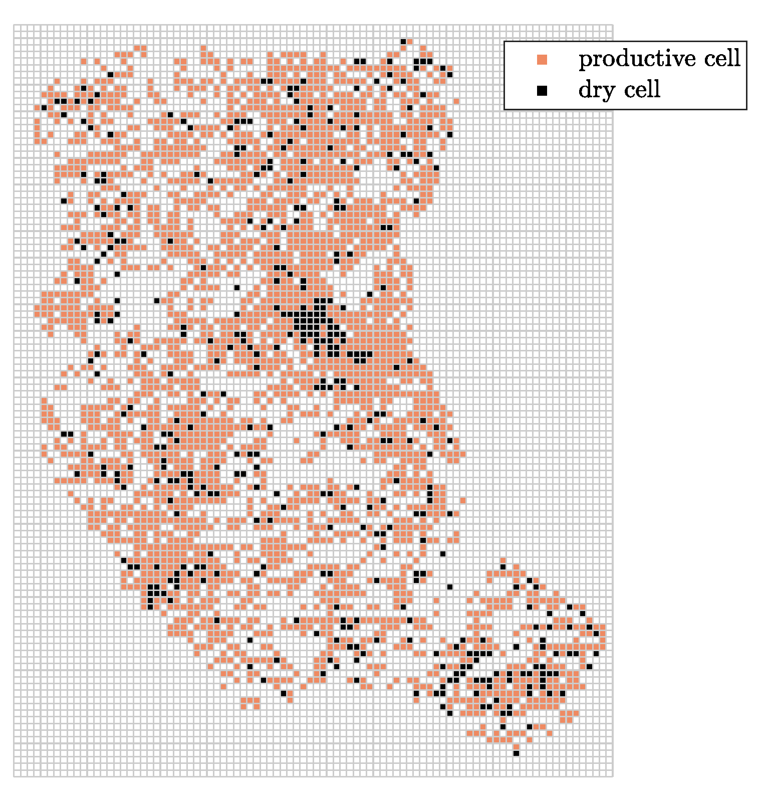
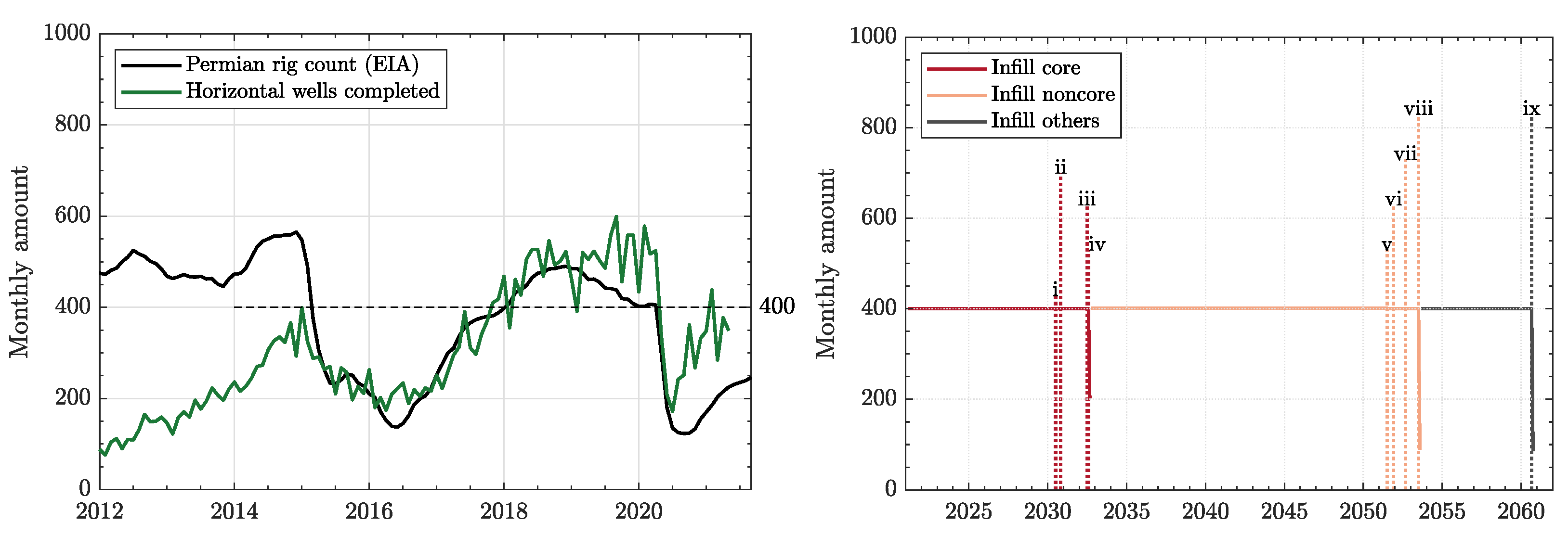
2.1. Design of Spatio-Temporal Well Cohorts

We start from identifying a minimum number of well cohorts in which oil production is statistically uniform. According to [5,8,9,10,11], these well cohorts need to be spatiotemporal because: (1) Production varies spatially throughout different reservoir layers and areas due to the geological variation of mudrock formations; and (2) it varies with completion dates because of the advancement of well technologies.

Figure 1 shows the areal extent of Permian Basin that spans an area of 75,000 square miles at the border between Texas and New Mexico. According to EIA [21], Permian Basin is further divided into several sub-basins: (1) the Central Basin Platform, that is the shallowest sub-basin, where the oldest vertical wells have been drilled since the 1930s; (2) the Midland Basin, which contains the tight Spraberry formation and Wolfcamp shale; (3) the Delaware Basin, which is the deepest sub-basin that contains the tight Bonespring formation and Wolfcamp shale; and (4) the Val Verde Basin, which produces an insignificant amount of oil and gas compared to the other three sub-basins. From USGS [6], we obtained the maximum extents of the major tight formations of the Permian age (290–275 million years ago): the Spraberry, Bonespring, and Wolfcamp in both Delaware and Midland Basins. In Figure 1, we also show a west-to-east vertical cut of the Permian Basin, cross-section (A-A${}^{\prime }$). We see that Spraberry in the Midland Basin is a shaly sandstone formation, relatively shallower compared with other major tight rocks. It consists of two main layers: the Upper and Lower Spraberry. Bonespring in the Delaware Basin is also a shaly sandstone formation, deeper than Spraberry. It consists of three main layers: the 1st, 2nd, and 3rd Bonespring. Lastly, Wolfcamp is a calcareous shale formation that exists in both Midland and Delaware basins. It is deeper and thicker than other major producing formations, and consists of four layers: Wolfcamp A, B, C, and D.

In Figure 2, we plot the maximum daily oil rates from the four major sub-regions of the Permian: (1) Delaware Bonespring; (2) Midland Spraberry; (3) Delaware Wolfcamp; and (4) Midland Wolfcamp. A Core area is an area that envelopes all best producing wells with the maximum daily oil rates of more than 750 bbl/d. We define each Noncore area as the difference between the core area and the formation extent defined by USGS.

From Figure 1 and Figure 2, we infer that well productivity varies across different sub-basins, and with reservoir layer depths. In addition, production in the Permian also varies with completion date intervals. We found that the newly completed wells produce at higher initial oil rates, but they decline faster. The production improvements among the new wells result from the advancements of completion technology in the Permian Basin. We observed similar trends in the Bakken [9], Haynesville [10], and Marcellus [11]. In Figure 3, we plot the mean, upper bound ($P_{10}$) and lower bound ($P_{90}$) of lateral lengths, fracturing water intensity, and proppant intensity. Over the last eight years, operators have drilled horizontal wells that are twice longer, and have doubled the amounts of hydraulic fracturing water and proppant per lateral foot.

Finally, we come up with a well classification shown in Figure 4 that divides all 53,708 horizontal wells into 36 well cohorts based on nine reservoir qualities and four completion date intervals. The first eight reservoir qualities are a combination of sub-basin, reservoir, and core-noncore divisions. All horizontal hydrofractured wells that do not fall into one of these categories are classified as the ninth reservoir quality: ‘Others’. The four completion date intervals are: (i) 2008–2013; (ii) 2014–2015; (iii) 2016–2017; and (iv) 2018–2021.

2.2. Physics-Based Data-Driven Well Prototypes

For each spatiotemporal well cohort in Figure 4, we first construct a historical well prototype using the Generalized Extreme Value (GEV) statistics. GEV is a generalization of the three extreme value distributions: Fréchet [12], Weibull [14], and Gumbel [13]. There are three parameters for a GEV distribution: the location parameter ($\mu$), the spread parameter ($\sigma$), and the shape parameter ($\xi$). The value of $\xi$ determines which of the three extreme distributions results, Fréchet ($\xi >0$), Weibull ($\xi <0$), and Gumbel ($\xi =0$). Using Equations (A1)–(A3), we calculate the probability density function (PDF), the cumulative distribution function (CDF), and the expected value or mean of the annual oil production of each well cohort for each $i\mathrm{th},i=1,\cdots ,n$-year on production. Figure 5 is an example of matching the annual production from 1269 horizontal hydrofractured wells with at least 1 year on production. These wells are completed in the Delaware Bonespring during 2008–2013. The shape factor $\xi$ is 0.1412, which yields a Fréchet distribution, typical of many other shale plays. The values of $\mu$ and $\sigma$ are shown as a contour plot of the 95% confidence interval (CI). From the cumulative density function (CDF) plot, we obtain $P_{10}$, $P_{50}$, and $P_{90}$. We overlay both GEV and lognormal fits on the empirical PDF to show the superiority of the GEV distribution in matching annual production in the Permian.

We continue to fit annual production from all horizontal wells in the Delaware Bonespring [2008–2013] with at least 2, 3,..., $t_N$ years on production, and record the mean, $P_{10}$, and $P_{90}$ values. The historical mean well prototype accumulates the recorded GEV means, shown as the thick black line in Figure 6. The $P_{10}$ and $P_{90}$ prototypes are also shown in Figure 6 as dashed lines. After we finish constructing the first historical well prototype; we repeat this process for the other 35 well cohorts in the Permian.

Next, as the obtained historical well prototypes are limited by the longest record of well data, we use our physical scaling (Physical scaling is a robust physics-based method of forecasting oil and/or gas production from the hydrofractured shale/tight formations. This method was first introduced in [15,16] for the Barnett shale, where it was shown that cumulative production from thousands of horizontal gas wells could be collapsed to an almost universal master curve. See Appendix B to learn more about physical scaling) that extrapolates the prototypes for several more decades. In Figure 6, we show the extrapolated well prototypes using physical scaling as the thick green lines. The corresponding fitting parameter, $\tau$, and the average-cohort estimated ultimate recovery (EUR) are tabulated in

Table 1. The fitted values of $\tau$’s and EUR’s for each well cohort. Note that each roman number represents different completion date intervals: (i). 2008–2013, (ii). 2014–2015, (iii). 2016–2017, (iv). 2018–2021.

Region	$\mathit{\tau }$ (Years)				EUR (kbbl/well)
	(i)	(ii)	(iii)	(iv)	(i)	(ii)	(iii)	(iv)
Delaware Bonespring Core	11.9	7.8	5.3	5.0	178	277	349	407
Delaware Bonespring Noncore	13.7	8.9	12.3	5.8	210	224	195	311
Midland Spraberry Core	7.2	6.1	5.2	5.0	87	314	327	299
Midland Spraberry Noncore	8.3	7.0	5.2	8.6	119	150	214	208
Delaware Wolfcamp Core	19.8	8.5	7.6	7.7	295	350	467	445
Delaware Wolfcamp Noncore	-	8.9	8.3	7.7	-	220	261	286
Midland Wolfcamp Core	6.7	6.2	5.2	6.0	137	215	325	316
Midland Wolfcamp Noncore	7.7	7.1	6.0	6.9	82	95	161	194
Others	12.9	10.1	7.5	5.2	137	201	209	229

for the 36 Permian well cohorts. We observe that both the Delaware Bonespring Core and the Delaware Wolfcamp Core give the highest EURs. This is because these two formations are thicker and more mature than those in the Midland Basin. On the other hand, the newer wells yield significantly higher EURs due to longer lateral lengths and bigger hydraulic fractures. However, in areas of poor reservoir quality, these advancements of completion technologies cannot help much.

In this study, we find that the GEV distribution can also be used to model the gas-oil ratios (GOR) and water cuts (WC) of the horizontal hydrofractured wells in the Permian. Figure 7 shows the GEV fits of GOR and WC from the Midland Spraberry Core and the Midland Wolfcamp Core. We observe that the shape factor, $\xi$, of the GOR fit is typically positive (Fréchet), while $\xi$ is negative for the WC (Weibull). The GEV means of GOR and WC for each Permian sub-region are listed in

Table 2. Summary of GEV-mean GOR and GEV-mean Watercut for each Permian region.

Region	Gas Oil Ratio (scf/stb)	Water Cut
Delaware Bonespring Core	3058	0.54
Delaware Bonespring Noncore	2809	0.64
Midland Spraberry Core	1574	0.59
Midland Spraberry Noncore	3949	0.51
Delaware Wolfcamp Core	3285	0.67
Delaware Wolfcamp Noncore	6965	0.70
Midland Wolfcamp Core	3019	0.52
Midland Wolfcamp Noncore	4430	0.57
Others	4385	0.63

. Following [17,22], we assume that: (1) hydrocarbon and water take different flow paths from the matrix to the hydrofracture network, (2) the flowing hydrocarbon is undersaturated, therefore no gas could escape from the oil solution. With these assumptions, we obtain mean well prototypes for gas as the mean well prototypes of oil multiplied by the expected values of GOR.

The well prototypes obtained from GEV statistics and physical scaling are highly idealized, and assume that de facto production from each well continues uninterrupted for several decades. The increase in water production, the reduction of reservoir pressure, the reduction of effective rock permeability, and well integrity problems are some of the reasons why operators shut-in their wells after less than 15 years on production. Therefore, we ought to calculate the maximum time on survival, $t_{max}$, that limits the durability of all wells represented by their prototypes. Figure 8 is an example from the Delaware Bonespring Core that shows why $t_{max}=10.8$ years from the data based well survival probabilities. We calculate the probability of well survival from Equation (A7). Finally,

Table 3. Summary of maximum survival time, probability of success, maximum well density, and infill potential for each Permian region.

Region	Survival Time (Years)	Probability of Success	Max. Density (wells/mi2)	Infill Potential
Delaware Bonespring Core	10.8	0.82	12	6946
Delaware Bonespring Noncore	8.7	0.82	12	28,425
Midland Spraberry Core	8.7	0.72	8	4712
Midland Spraberry Noncore	7.3	0.76	8	18,681
Delaware Wolfcamp Core	11.0	0.79	16	17,550
Delaware Wolfcamp Noncore	9.7	0.79	12	32,780
Midland Wolfcamp Core	10.0	0.87	16	26,195
Midland Wolfcamp Noncore	9.2	0.75	12	20,429
Others	8.6	0.33	4	34,086

summarizes the values of $t_{max}$ for all Permian sub-regions. Typically, the core area wells survive longer than the noncore area wells, as also observed for other shale plays.

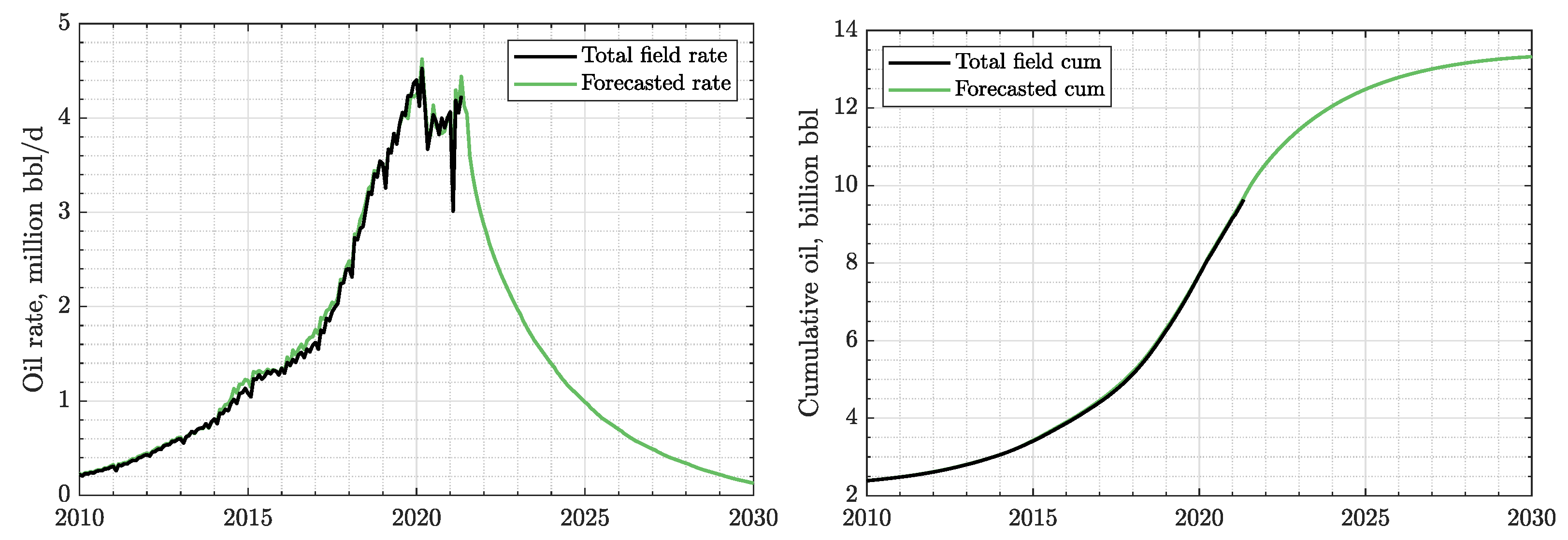
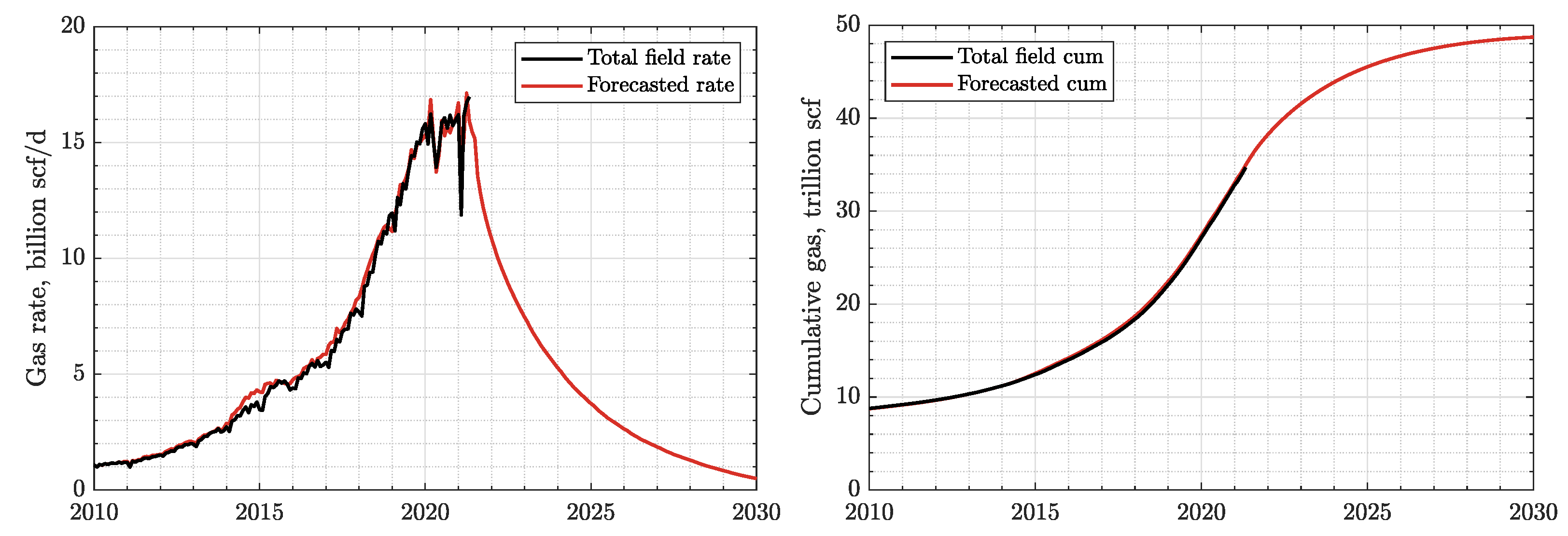
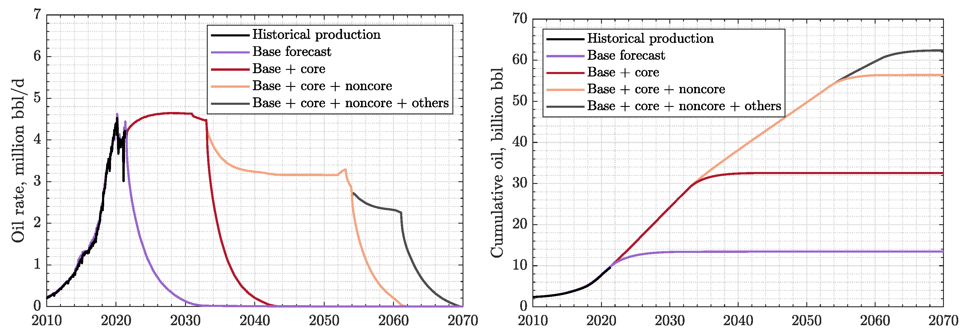
2.3. Production Forecast

We replace the production rate history from each existing horizontal hydrofractured well in the Permian with its corresponding well prototype time-shifted to the calendar date of first well production, and sum the prototypes up. Our well prototypes are robust, so that in Figure 9, the summation of prototypes (green line) matches the historical production (black line) with high fidelity. The green line extrapolates the total production rate for several more decades. This projection is what we call ‘base’ or ‘do-nothing’ forecast, which is the most pessimistic scenario assuming that the future production will only come from the existing wells. If all operators stopped drilling new wells, today’s production would reduce by half in just two years. Unfortunately, this fast decline of production rate is typical of every shale/tight play development. From the cumulative production plot, we estimate that all 53,708 existing horizontal wells in the Permian will ultimately produce 13.4 billion bbl of oil by 2030.

On the other hand, gas production in the Permian is substantial, as evidenced by its second rank among all tight gas producers in the U.S. We, therefore, perform a similar forecast for gas output of the Permian. Similar to the oil base forecast, we replace gas rates from each existing well in Permian with their prototypes, and multiply with the GEV mean GOR before it is time-shifted to the first production date. Again, the summation of prototypes closely matches the historical gas production, showing the robustness of GEV statistics. Figure 10 shows the ‘base’ forecast for gas as red lines. In a ‘do-nothing’ scenario, Permian will ultimately produce 48.5 trillion scf of gas by 2030.

Before we proceed to estimate future production from infill drilling projects, we need to calculate the infill potential of each sub-region of the Permian. Figure 11 shows two snapshots from Google Earth of some of the densest drilled areas in Loving County, Texas (a part of the Delaware Basin) and Upon County, Texas (a part of the Midland Basin). Both views are overlaid with the $1\times 1$ mi${}^2$ (≈$1609\times 1609$ m${}^2$) squares rotated to fit wellhead patterns. The rotation is 0${}^{\circ }$ for Loving county and 16${}^{\circ }$ for Upon County. In both areas, the well density is exactly 16 wells per sq mi, which is much higher than what we observe in other U.S. shale plays. If we look again at Figure 1, we see that the Permian is a basin with multiply stacked reservoirs. For instance, in the Delaware Basin, operators can drill from the same wellpad into three layers of the Bonespring plus four layers of the Wolfcamp. This advantage does not exist in other major U.S. shale plays.

In Figure 12, we demonstrate how we calculate the infill potential using the Midland Spraberry Core as an example. We first create two blank cell grids with a size of one square-mile. We start by filling the first cell grid with all 2492 existing horizontal wells completed in the Midland Spraberry Core. Notice that the direction of lateral sections follows the tilt of horizontal wells in Upton County in Figure 11. Typically, wells are drilled horizontally along minimum horizontal stress (in this case ∼S${16}^{\circ }$ E), so that we obtain optimal hydraulic fractures that grow in the direction of maximum horizontal stress. We then count the number of horizontal wells that intersect each cell as horizontal well density. We also fill the second grid with 25,510 existing vertical wells in the Midland Spraberry Core, and count the number of vertical wells in each cell as vertical well density. Using Equation (A10), we calculate the infill potential as the maximum well density to prevent frac hits, minus the horizontal well density, minus the vertical well density scaled by the r-parameter (we assume that the drainage area of a vertical well is r times less than that of a horizontal well. In a separate paper [5], we establish that EUR of new vertical wells in the Permian is roughly the same at 50 kbbl/well for all reservoir ages and areas of the Permian. Therefore we approach r as the ratio between EUR of a horizontal well (previously calculated in Table 1) and the EUR of a vertical well, which is 50 kbbl/well.). In Table 3, we summarize the infill potential for each region of Permian.

To obtain a more realistic number of future producing wells, we multiply the infill potential with the probability of success, $P_{\mathrm{success}}$ that is defined as a probability of successfully finding the non-dry (productive) wells. As an example, we show the spread of dry (black) and productive (orange) cells in the Midland Wolfcamp Core in Figure 13. The values of $P_{\mathrm{success}}$ for all Permian sub-regions is summarized in Table 3. We observe that $P_{\mathrm{success}}$ is about 0.8 for all major core and noncore Permian tight formations, except for the ‘Others’ region where the reported $P_{\mathrm{success}}$ is as low as 0.33.

Next, we schedule the most probable drilling programs based on the infill potential calculated in the previous section. In 2012, there was a big discrepancy between horizontal wells completed and rig count because: (1) Operators still aimed to drill vertical wells in some conventional reservoirs in the Permian; and (2) The completion technology for horizontal wells at that time was not as good as it is today. Since 2015, the rig count has matched closely the horizontal wells completed, indicating that operators no longer drill many vertical wells. The horizontal wells completed during the COVID-19 pandemic crisis deviated significantly from the rig count, because operators did not have money to maintain the same drilling pace. Therefore, they chose to complete the drilled but uncompleted wells (DUC) that are numerous in the Permian compared with other U.S. shale plays. Based on the historical drilling rate, we choose 400 wells per month as a base for future drilling schedule.

Figure 14 (right) shows the future drilling programs in the Permian. We assume that operators will drill in the core area first, exhausting potential locations by 2032. When no drilling spots are left in the core areas, operators will move to the less productive noncore areas and drill the same number of horizontal wells until 2053. Finally, no drilling spots will be left in the Bonespring, Spraberry, or Wolfcamp in the Midland and Delaware basins, and operators will drill the least productive ‘Others’ area until 2060. We need to highlight that the last drilling program is unlikely. Next, we will show that the ‘Others’ area is profitable only when the oil price is very high.

Using the same well prototypes in Figure 6 and GOR values in Table 3, we obtain the infill forecasts for oil production (Figure 15) and gas production (Figure 16). In Figure 15 (left), we show that by drilling new 55,402 horizontal wells in the core areas, we can maintain the production plateau of 4.6 million bbl/d for one more decade. Drilling additional 100,314 wells in the less productive noncore areas will drop the future oil rate plateau to 3.2 million bbl/d until 2053. Drilling 34,086 wells in the ‘Others’ area will not save the Permian Basin from terminal decline. The cumulative production in Figure 15 (right) shows the estimated ultimate recovery (EUR) for each infill scenario. Recall that the existing wells will ultimately produce 13 million bbl. By adding future drilling in the core, noncore, and ‘Others’ area, the oil EUR will increase to 32.2, 54.4, and 62.4 million bbl, respectively.

The forecast of future gas production is shown in Figure 16. Drilling core areas will maintain the gas rate plateau at about 17 billion scf/d until 2033. Interestingly, as the noncore areas mostly contain much more gas than the core areas, the gas rate plateau will increase to 18 billion scf/d. Finally, the gas EUR for existing wells in the Permian is about 50 trillion scf. By adding the Core, Noncore, and ‘Others’ area, the gas EUR will increase to 120, 246, and 285 trillion scf, respectively. Recalling our analysis for the Marcellus [11], we posit that the Permian Basin will soon surpass the giant Marcellus shale in terms of gas rate and technically recoverable gas.

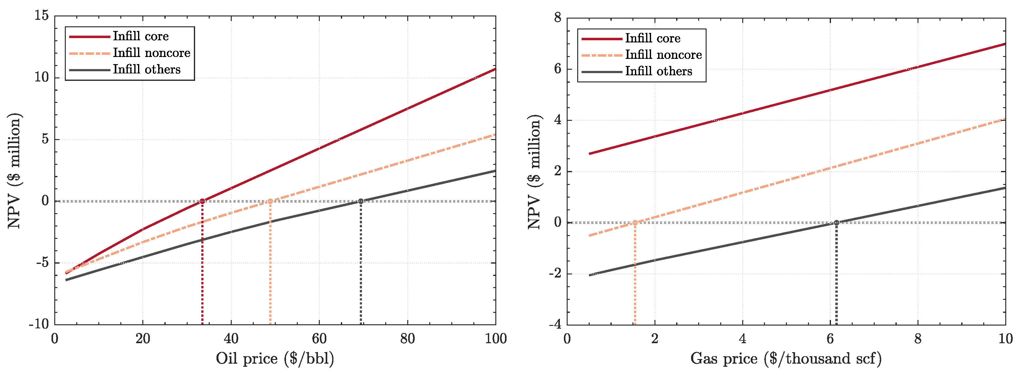
2.4. Economic Analysis

To evaluate the profitability of each drilling program, we perform a robust economic analysis that calculates and compares the net present values (NPV) of each project (

Table 4. Parameters used to calculate NPV in the Permian basin.

Parameters	Notations	Units	Values	Notes
Drilling & comp. cost	DRILL	$ million	6.0	Delaware Bonespring ${}^{\left(a\right)}$
			6.4	Midland Spraberry ${}^{\left(a\right)}$
			8.9	Delaware Wolfcamp ${}^{\left(b\right)}$
			7.0	Midland Wolfcamp ${}^{\left(a\right)}$
			6.9	Others ${}^{\left(c\right)}$
Land acquisition cost	LAND	$ million	0.5	${}^{\left(d\right)}$
Plug & abandon. cost	PLUG	$ million	0.3	${}^{\left(e\right)}$
Operating cost	OPEX	$/bbl	0.7	Oil ${}^{\left(b\right)}$
		$/bbl	0.5	Water ${}^{\left(b\right)}$
		$/kscf	0.1	Gas ${}^{\left(b\right)}$
Severance tax rate	TAXS	$/kscf	0.05	${}^{\left(a\right)}$
Corporate tax rate	TAXC	frac./year	0.25	${}^{\left(f\right)}$
Intangible expend.	INTAN	frac./year	0.5
Royalty rate	ROY	frac./year	0.15	${}^{\left(b\right)}$
Discount rate	DIS	frac./year	0.08	${}^{\left(a\right)}$

Sources: ${}^{\left(a\right)}$ [23], ${}^{\left(b\right)}$ [24], ${}^{\left(c\right)}$ [25], ${}^{\left(d\right)}$ [26], ${}^{\left(e\right)}$ [27], ${}^{\left(f\right)}$ [28].

). We adopt our previous NPV formulation for gas wells in the Haynesville and Marcellus [11,18], and change several parameters to accommodate the significant gas and water production in the Permian Basin. See Appendix D for the full methodology of calculating NPV.

Figure 17 summarizes the results of our economic analyses for three different infill scenarios: Core, Noncore, and ‘Others’ in the Permian Basin. We plot the net present value (NPV) versus the prices. If NPV is positive, the project is profitable and vice versa. The intercept between each NPV line and the line $\mathrm{NPV}=0$ is called the break-even point that indicates the oil/gas prices, below which an infill project becomes unprofitable. Figure 17 (left) shows a scenario where we assume a constant gas price of $4/kscf and vary the oil prices. We observe that infilling core areas is profitable even if the oil price is as low as $35/bbl. Infilling noncore areas is only profitable if the oil price exceeds $52/bbl. Operators should avoid infilling the ‘Others’ area, unless the oil price is above $72/bbl. The second scenario is shown in Figure 17 (right) where we assume a constant oil price of $60/bbl and vary gas prices. Using this scenario, infilling core areas will be profitable at any gas price. The break-even points for infilling the noncore and ‘Other’ areas are $1.5/kscf and $6/kscf.

In

Table 5. Summary of crude oil resources in the Permian tight reservoirs.

Region	Existing	Remaining Resources			Est. Ultimate Recovery
	Wells	${\mathit{P}}_{10}$	Mean	${\mathit{P}}_{90}$	${\mathit{P}}_{10}$	Mean	${\mathit{P}}_{90}$
	(Gbbl)	(Gbbl)	(Gbbl)	(Gbbl)	(Gbbl)	(Gbbl)	(Gbbl)
Delaware Bonespring Core	1.0	4.6	3.0	1.1	5.6	4.0	2.1
Delaware Bonespring Noncore	0.2	14.8	8.3	2.7	15.0	8.5	2.9
Midland Spraberry Core	1.6	2.2	1.6	0.5	3.8	3.2	2.2
Midland Spraberry Noncore	0.6	9.8	3.4	0.6	10.4	3.9	1.2
Delaware Wolfcamp Core	2.4	12.5	8.8	3.0	14.9	11.2	5.3
Delaware Wolfcamp Noncore	0.1	16.2	8.7	2.7	16.3	8.8	2.7
Midland Wolfcamp Core	2.3	13.8	8.7	2.5	16.1	11.0	4.8
Midland Wolfcamp Noncore	0.1	8.2	3.7	0.6	8.3	3.8	0.7
Others	1.6	12.5	6.3	0.8	14.1	7.9	2.4
TOTAL	9.9	94.6	52.5	14.5	104.5	62.4	24.4
TOTAL Core + Noncore	8.3	82.2	46.2	13.7	90.4	54.4	22.0

and

Table 6. Summary of natural gas resources in the Permian tight reservoirs.

Region	Existing	Remaining Resources			Est. Ultimate Recovery
	Wells	${\mathit{P}}_{10}$	Mean	${\mathit{P}}_{90}$	${\mathit{P}}_{10}$	Mean	${\mathit{P}}_{90}$
	(Tscf)	(Tscf)	(Tscf)	(Tscf)	(Tscf)	(Tscf)	(Tscf)
Delaware Bonespring Core	4.0	16.8	10.5	4.2	20.8	14.5	8.1
Delaware Bonespring Noncore	0.5	50.0	27.8	9.2	50.4	28.3	9.7
Midland Spraberry Core	3.7	4.1	3.1	1.0	7.8	6.8	4.7
Midland Spraberry Noncore	2.4	46.5	16.0	2.9	48.9	18.4	5.2
Delaware Wolfcamp Core	11.0	49.4	33.9	11.7	60.4	44.9	22.6
Delaware Wolfcamp Noncore	0.8	135.4	72.6	22.2	136.2	73.4	23.0
Midland Wolfcamp Core	7.0	50.1	32.5	9.0	57.1	39.5	16.0
Midland Wolfcamp Noncore	0.5	43.4	19.8	3.0	43.9	20.3	3.6
Others	5.9	65.7	33.1	4.3	71.5	39.0	10.2
TOTAL	35.7	461.5	249.3	67.5	497.2	285.0	103.2
TOTAL Core + Noncore	29.8	395.8	216.2	63.2	425.6	246.1	93.0

, we recapitulate the existing production, remaining resources, and the estimated ultimate recoveries of oil and gas in the Permian Basin, based on our study. We highlight the difference between the resources if we neglect the least profitable ‘Others’ area. On the one hand, our prediction of total recoverable oil of 54.4–62.4313 billion bbl falls in-between what USGS and EIA predict at 46 and 95.6 billion bbl, respectively. On the other hand, we predict that the total recoverable gas is between 246–285 trillion scf, which is close to the predictions from USGS and EIA at 280 and 284.8 trillion scf.

3. Discussion

We have presented an optimal play-wide assessment of the Permian tight reservoirs by considering not only the play geology, but also the advancements of well completion technologies, physics of hydrocarbon production from the horizontal hydrofractured wells subject to attrition, and economics of drilling projects. Our physics-based, data-driven well prototypes are robust and able to match accurately the historical oil and gas production from the entire Permian play. By comparing these well prototypes, we observe that wells completed in the Delaware Basin give higher EURs than those in the Midland Basin. One can postulate that during the Permian, 298–252 million years ago, the Delaware was located deeper than the Midland. Thus, the tight carbonate and shale deposits in the Delaware Basin that we find today are thicker than those in the Midland Basin. As downhole temperature increases with depth, we also expect that the Bonespring and Wolfcamp formations in the Delaware Basin are more mature and produce more hydrocarbons than the Spraberry and Midland formations in the Midland Basin.

Similar with our findings in other tight/shale plays (Barnett [8], Eagle Ford [17], Bakken [9,18], Haynesville [10], and Marcellus [11]), we learn that the best wells are located only within the relatively small ‘sweet-spot’ or core areas, which are barely 10–45% of the total formation extents. The remaining noncore and outer areas tend to be immature and thin, so and they produce less than the core areas. We also show (by comparing well prototypes) that the newly completed wells are more productive than the old ones—if and only if they are drilled and completed in the best core areas. Advancement of drilling and completion technologies, that is, the longer lateral lengths and more of larger hydrofractures, will not help the operators to produce more from the lowest quality reservoirs. In addition, our economic analysis shows that drilling in the core areas is always profitable even if the oil price is as low as $35/bbl, and at any gas price. The noncore and outer areas are unprofitable, unless the oil and gas prices are really high.

Finally, we estimate that the total recoverable oil in the Permian tight reservoirs is 54.4–62.4 billion bbl (Table 5), and the total recoverable gas is 246–285 trillion scf (Table 6). We posit that the Permian will continue to be the most prolific oil province in the U.S. for the next three or four decades. The Permian will also surpass the declining giant Marcellus shale as the top U.S. producer of natural gas. By now, operators in the Permian Basin should realize how priceless the good Permian wells are. They should not recklessly over-drill or over-fracture the core areas to earn a fast buck. Instead, they should maintain reservoir performance in the existing depleted areas to deliver secure oil and gas production that will subsidize a future which might lead to a ‘clean’ energy transition.

4. Materials and Methods

We gathered public-domain well data from the FracFocus and Enverus databases. Our dataset consists of 562,416 wells completed in the Permian Basin (Texas and New Mexico). In this paper, we analyzed production from only 53,708 horizontal hydrofractured wells that were completed in major tight formations in the Midland or Delaware sub-basins of the Permian. Production from the other 484,759 vertical wells was analyzed in a separated paper [5].

We have summarized how to obtain economic production forecasts from the major Permian tight formations in Figure 18. The methodology used in this paper is based substantially on our prior work on the physics-guided, data-driven forecasts in the Barnett [8], Eagle Ford [17], Bakken [9,18], Haynesville [10], and Marcellus [11]. Very briefly, our approach is as follows:

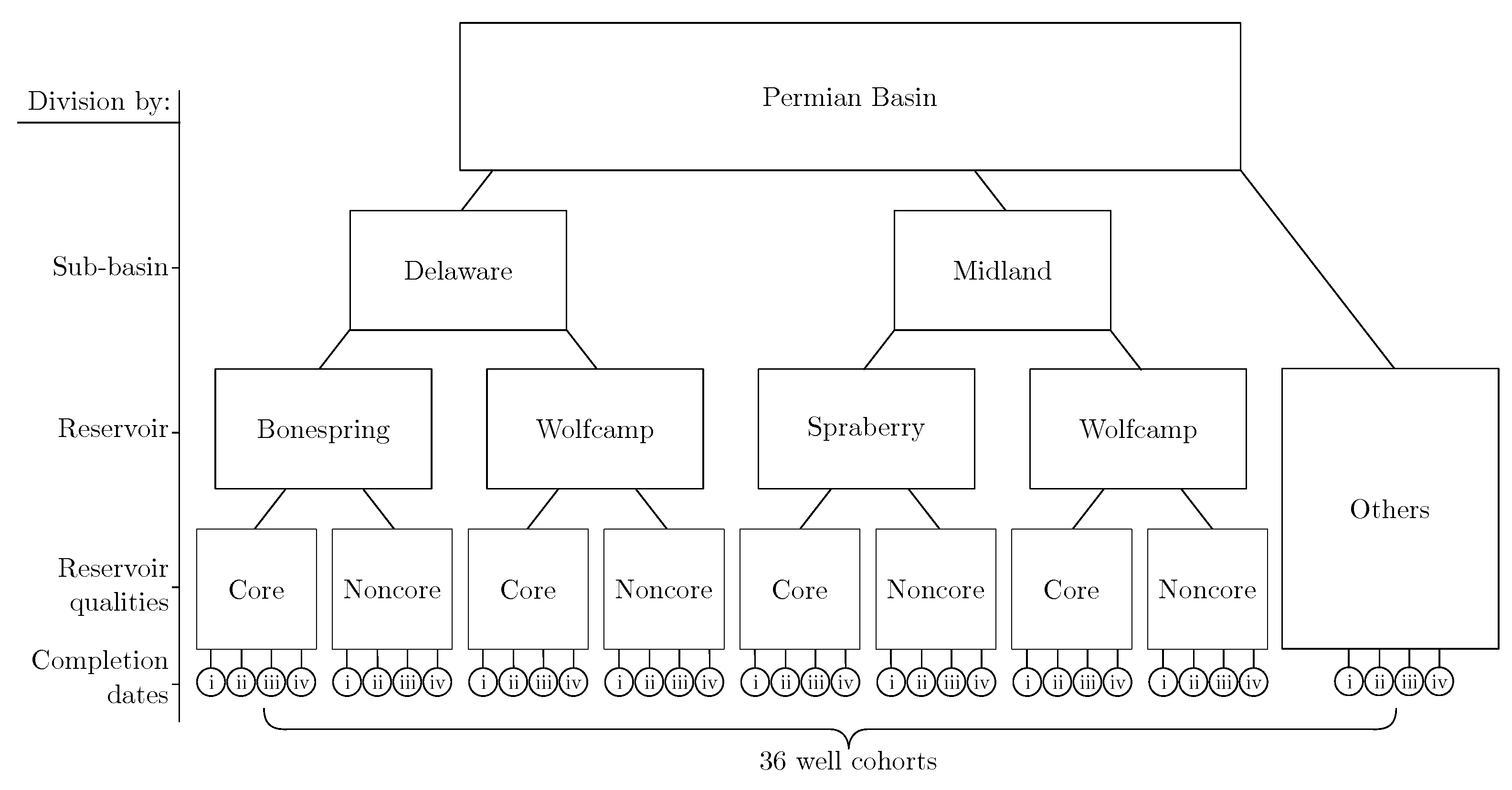
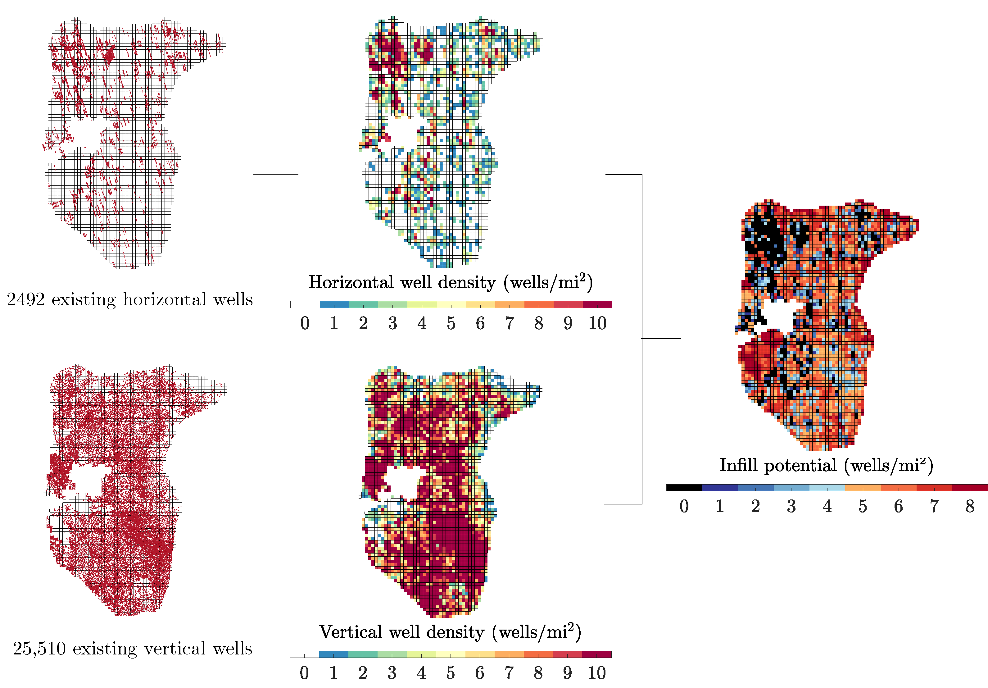
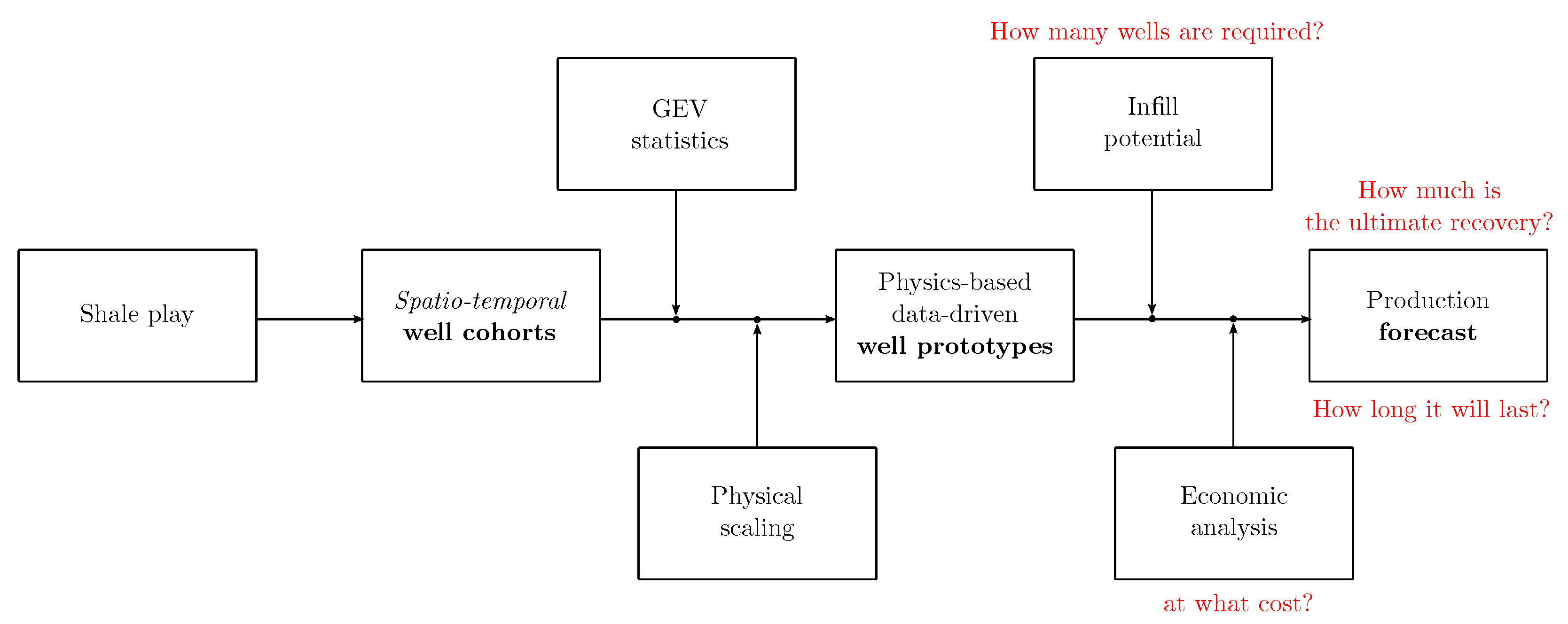
• We divide all 53,708 horizontal hydrofractured tight oil wells in the Permian into 36 spatiotemporal well cohorts, in which oil production is statistically uniform. The number 36 is the product of nine reservoir qualities and four completion date intervals;
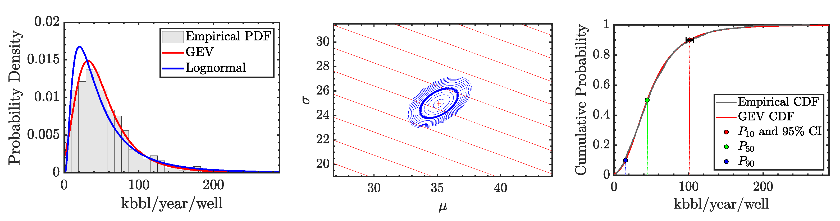
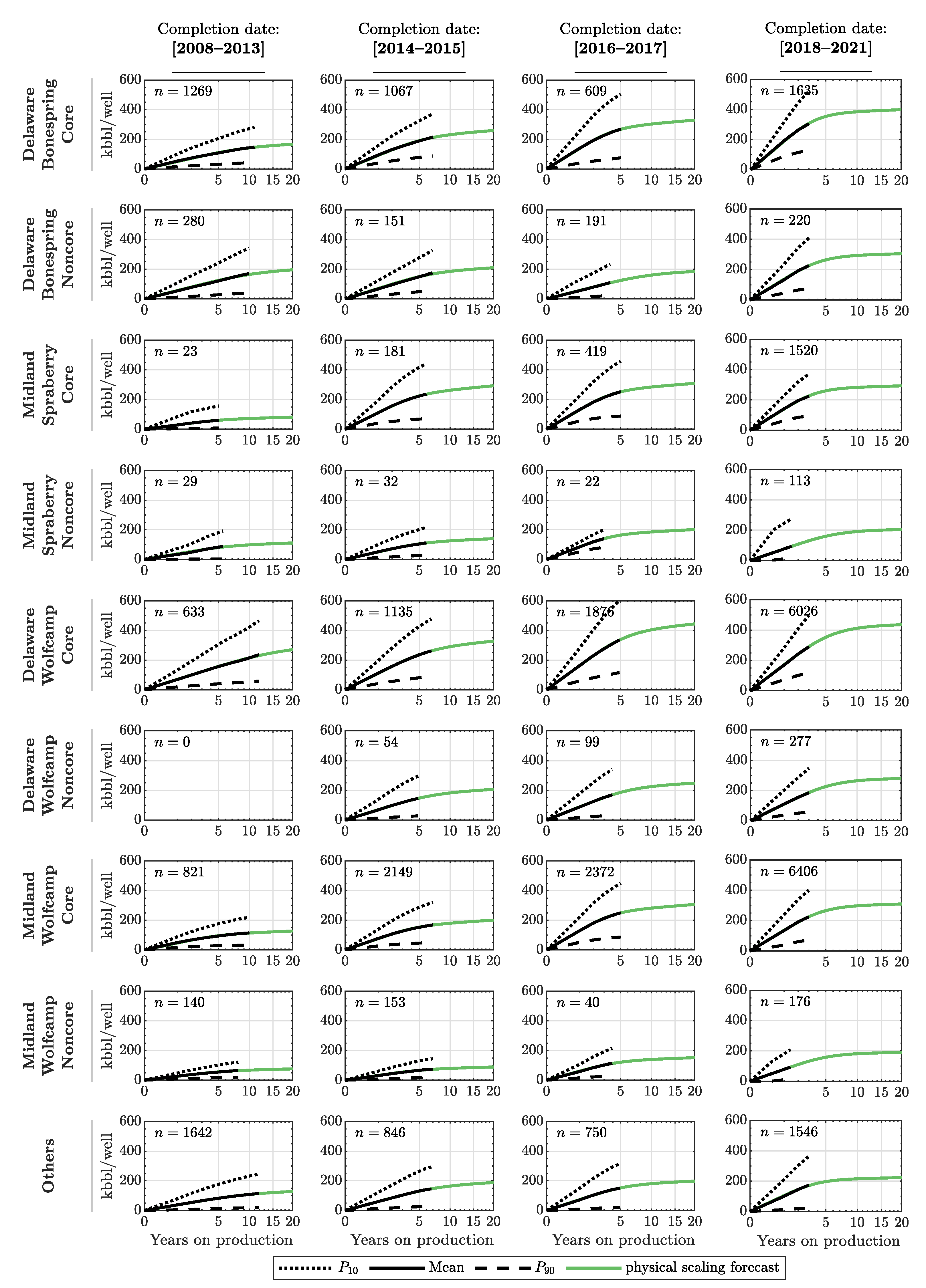
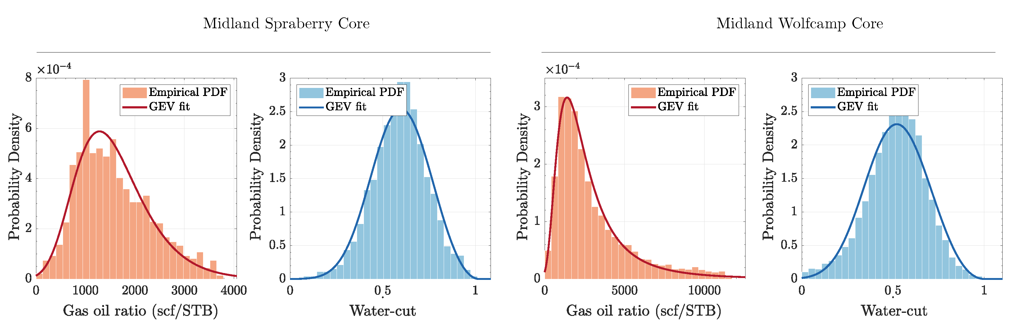
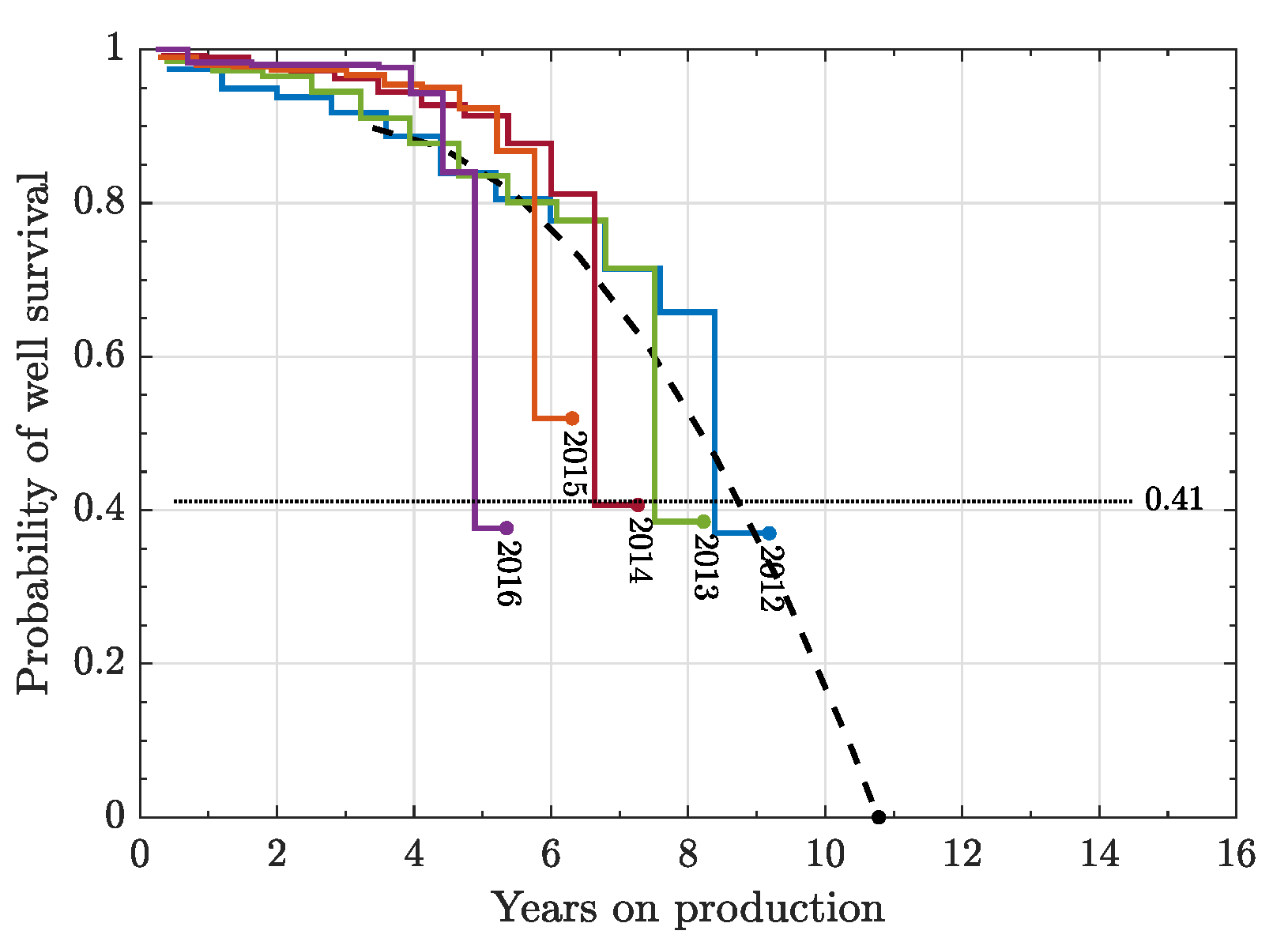
• For each cohort, we sample each oil of oil production of its wells and fit the resulting empirical distribution with a generalized extreme value (GEV) distribution, see Appendix A. We construct historical well prototypes as the expected (mean) values of the annual GEV distribution. Next, we use physical scaling to extrapolate the prototypes for several more decades, see Appendix B. We determine the data-driven well survival probabilities to make our prototypes even more realistic, see Appendix C;
• We replace the actual field production rate from all existing groups of wells in the Permian with their corresponding well prototypes. The summation of all the prototypes is now the ‘base’ or ‘do-nothing’ forecast of the Permian tight oil wells. To obtain the infill forecasts, we first calculate the probability of success and infill potential (see Appendix C). Then, we schedule future drilling programs. We calculate the net present value (NPV) (see Appendix D) to evaluate the profitability of each future drilling program.

5. Conclusions

• We have provided an optimal play-wide assessment of the Permian tight reservoirs by considering play geology, advancement of well completion technologies, physics of hydrocarbon production from the horizontal hydrofractured wells, well attrition, and economics of drilling projects;
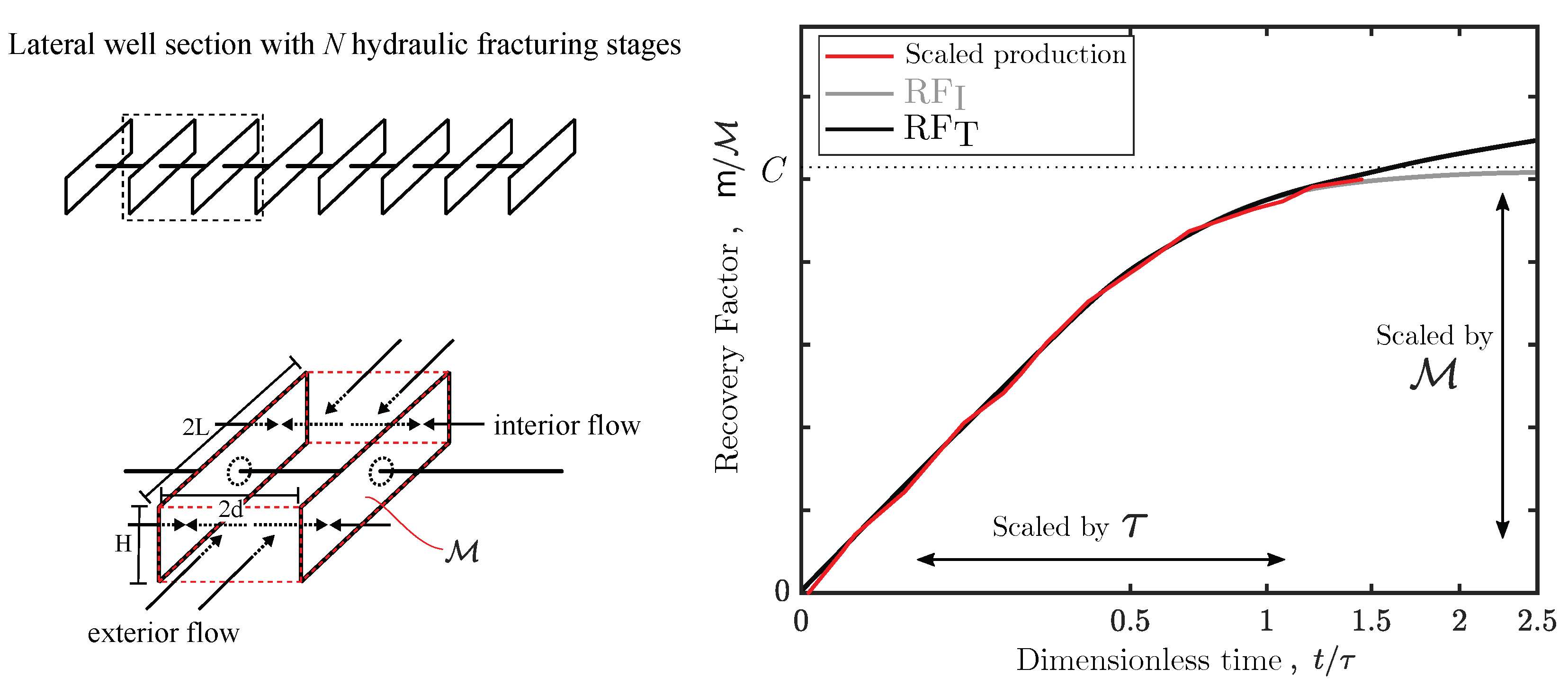
• Our mean Generalized Extreme Value statistics well prototypes are robust and in excellent agreement with the physics-based scaling curves. Using these prototypes, we were able to match rather well the historical oil and gas production from the entire Permian Basin;
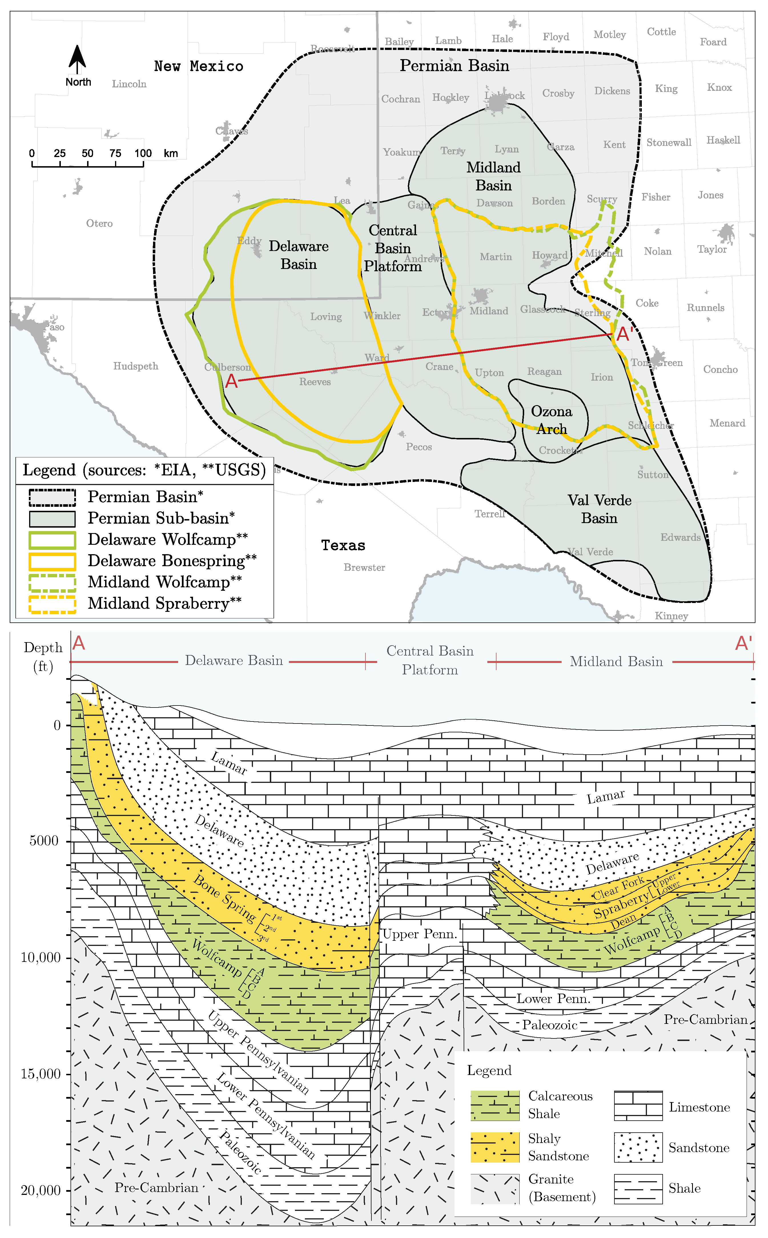
• Both the Delaware Bonespring Core and the Delaware Wolfcamp Core give the highest estimated ultimate recovery, because these two formations are thicker and more mature than those in the Midland Basin;
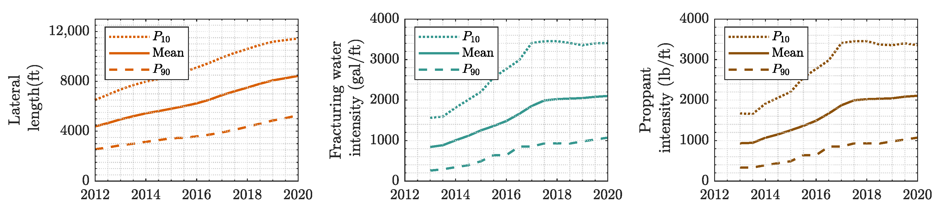
• The newer wells yield significantly higher EURs due to longer laterals and bigger hydraulic fractures. However, in areas of poor reservoir quality, these advancements of completion technologies do not help much;
• We estimate that the total recoverable oil in the Permian tight reservoirs is 54.4–62.4 billion bbl, and the total recoverable gas is 246–285 trillion scf;
• Operators might consider abstaining from drilling in the ‘Others’ area of the Permian, because it may be unprofitable for all scenarios we considered;
• It is most likely that Permian will continue to be the most prolific oil play in the U.S. and will surpass the declining giant Marcellus shale in producing natural gas. However, we should not assume that hydrocarbon production from the Permian will last for centuries and keep on subsidizing our energy demands.

References

1. Fox, K. The Energy Crisis Couldn’t Have Come at a Worse Time for Climate. 2021. Available online: https://edition.cnn.com/2021/10/08/business/energy-crisis-climate-fossil-fuels-renewables-cop26-cmd-intl/index.html (accessed on 10 October 2021).
2. Looney, B. Statistical Review of World Energy 2021, 70th ed.; BP Statistical Review: London, UK, 2021; Volume 70, p. 66. [Google Scholar]
3. Nalley, S.; LaRose, A.; Energy Information Administration (EIA). International Energy Outlook 2021 (IEO2021); Energy Information Administration (EIA): Washington, DC, USA, 2021; Volume 10, p. 9. [Google Scholar]
4. Nalley, S.; LaRose, A.; Energy Information Administration (EIA). Annual Energy Outlook 2021(AEO2021): Petroleum and other liquids. In Annual Energy Outlook; US Energy Information Administration: Washington, DC, USA, 2021; Volume 2, p. 4. [Google Scholar]
5. Saputra, W.; Kirati, W.; Patzek, T.W. Generalized extreme value statistics, physical scaling and forecasts of oil production from all vertical wells in the Permian Basin. Energies 2021. submitted. [Google Scholar]
6. Gaswirth, S.B.; French, K.L.; Pitman, J.K.; Marra, K.R.; Mercier, T.J.; Leathers-Miller, H.M.; Schenk, C.J.; Tennyson, M.E.; Woodall, C.A.; Brownfield, M.E.; et al. Assessment of Undiscovered Continuous Oil and Gas Resources in the Wolfcamp Shale and Bone Spring Formation of the Delaware Basin, Permian Basin Province, New Mexico and Texas, 2018; US Geological Survey: Reston, VA, USA, 2018. [Google Scholar] [CrossRef]
7. Nalley, S.; LaRose, A.; Energy Information Administration. Assumptions to the Annual Energy Outlook 2021: Oil and Gas Supply Module. In Annual Energy Outlook; US Energy Information Administration: Washington, DC, USA, 2021; p. 4. [Google Scholar]
8. Patzek, T.W.; Saputra, W.; Kirati, W.; Marder, M. Generalized Extreme Value Statistics, Physical Scaling, and Forecasts of Gas Production in the Barnett Shale. Energy Fuels 2019, 33, 12154–12169. [Google Scholar] [CrossRef]
9. Saputra, W.; Kirati, W.; Patzek, T. Generalized Extreme Value Statistics, Physical Scaling and Forecasts of Oil Production in the Bakken Shale. Energies 2019, 12, 3641. [Google Scholar] [CrossRef] [Green Version]
10. Saputra, W.; Kirati, W.; Patzek, T.W. Generalized extreme value statistics, physical scaling and forecasts of gas production in the Haynesville shale. J. Nat. Gas Sci. Eng. 2021, 94, 104041. [Google Scholar] [CrossRef]
11. Saputra, W.; Kirati, W.; Hughes, D.; Patzek, T.W. Forecast of Economic Gas production in the Marcellus. AAPG Bull. 2021. accepted. [Google Scholar]
12. Fréchet, M. Sur la loi de probabilité de l’écart maximum. Ann. Soc. Math. Polon. 1927, 6, 93–116. [Google Scholar]
13. Gumbel, E.J. Statistical theory of extreme values and some practical applications. NBS Appl. Math. Ser. 1954, 33., 19–33. [Google Scholar]
14. Weibull, W. A statistical distribution function of wide applicability. J. Appl. Mech. 1951, 18, 293–297. [Google Scholar] [CrossRef]
15. Patzek, T.W.; Male, F.; Marder, M. From the Cover: Cozzarelli Prize Winner: Gas production in the Barnett Shale obeys a simple scaling theory. Proc. Natl. Acad. Sci. USA 2013, 110, 19731–19736. [Google Scholar] [CrossRef] [PubMed] [Green Version]
16. Patzek, T.W.; Male, F.; Marder, M. A simple model of gas production from hydrofractured horizontal wells in shales. AAPG Bull. 2014, 98, 2507–2529. [Google Scholar] [CrossRef]
17. Patzek, T.W.; Saputra, W.; Kirati, W. A Simple Physics-Based Model Predicts Oil Production from Thousands of Horizontal Wells in Shales. In Proceedings of the SPE Annual Technical Conference and Exhibition, San Antonio, TX, USA, 9–11 October 2017. [Google Scholar]
18. Saputra, W.; Kirati, W.; Patzek, T. Physical Scaling of Oil Production Rates and Ultimate Recovery from All Horizontal Wells in the Bakken Shale. Energies 2020, 13, 2052. [Google Scholar] [CrossRef] [Green Version]
19. Arps, J. Analysis of Decline Curves. Trans. AIME 1945, 160, 228–247. [Google Scholar] [CrossRef]
20. Saputra, W.; Albinali, A.A. Validation of the Generalized Scaling Curve Method for EUR Prediction in Fractured Shale Oil Wells. In Proceedings of the SPE Kingdom of Saudi Arabia Annual Technical Symposium and Exhibition, Dammam, Saudi Arabia, 23–26 April 2018. [Google Scholar]
21. EIA. Maps: Oil and Gas Exploration, Resources, and Production; US Energy Information Administration: Washington, DC, USA, 2021. [Google Scholar]
22. Male, F. Using a segregated flow model to forecast production of oil, gas, and water in shale oil plays. J. Pet. Sci. Eng. 2019, 180, 48–61. [Google Scholar] [CrossRef]
23. Berman, A. Giant Wolfcamp Oil Field Would Lose $500 Billion at Today’s Prices. 2016. Available online: https://www.forbes.com/sites/arthurberman/2016/11/20/permian-giant-oil-field-would-lose-500-billion-at-todays-prices/ (accessed on 1 October 2021).
24. Xiong, H.; Ramanthan, R.; Nguyen, K. Maximizing Asset Value by Full Field Development—Case Studies in the Permian Basin. In Proceedings of the 7th Unconventional Resources Technology Conference, Brisbane, Australia, 18–19 November 2019; American Association of Petroleum Geologists: Tulsa, OK, USA, 2019. [Google Scholar]
25. Equity, O.G. Drilling & Completion Facts. 2021. Available online: https://www.oilgasequity.com/resources/drilling-completion-facts/ (accessed on 1 October 2021).
26. EIA. Trends in US Oil and Natural Gas Upstream Costs; US Energy Information Administration: Washington, DC, USA, 2016. [Google Scholar]
27. Observer, G. Abandoned Oil Gas Wells Permian Texas-New Mexico. 2021. Available online: https://grist.org/abandoned-oil-gas-wells-permian-texas-new-mexico/ (accessed on 1 October 2021).
28. Gentile, N. Federal Oil and Gas Royalty and Revenue Reform. 2021. Available online: https://www.americanprogress.org/issues/green/reports/2015/06/19/115580/federal-oil-and-gas-royalty-and-revenue-reform/ (accessed on 1 October 2021).
29. Eftekhari, B.; Marder, M.; Patzek, T.W. Field data provide estimates of effective permeability, fracture spacing, well drainage area and incremental production in gas shales. J. Nat. Gas Sci. Eng. 2018, 56, 141–151. [Google Scholar] [CrossRef]
Figure 1. Aerial extents and cross-section of Permian Basin, sub-basins, and the most prolific producing tight formations: Wolfcamp, Bonespring and Spraberry. Data sources: EIA [21] and USGS [6].
Energies 15 00043 g001
Figure 2. Production data-driven definition of core and noncore areas for the four Permian tight reservoirs: Delaware Bonespring, Midland Spraberry, Delaware Wolfcamp, and Midland Wolfcamp. The outer outline was obtained from USGS and is consistent with Figure 1.
Energies 15 00043 g002
Figure 3. Advancement of drilling and completion technologies in the Permian. Lateral lengths, fracturing water intensity, and proppant intensity have increased more than two-fold over the last eight years.
Energies 15 00043 g003
Figure 4. The 53,708 horizontal wells completed in the Permian tight reservoirs are divided into 36 well cohorts based on reservoir quality and completion date intervals.
Energies 15 00043 g004
Figure 5. Example of fitting the first year on production of a well cohort in the Delaware Bonespring [2008–2013] with a Generalized Extreme Value (GEV) distribution. From this match, ξ = 0.1412 , μ = 35.12 , and σ = 24.97 .
Energies 15 00043 g005
Figure 6. The black lines show the historical mean, upper bound ( P 10 ), and lower bound ( P 90 ) from the GEV statistics of the 36 well cohorts in the Permian Basin. The green lines are the extended well prototypes from physical scaling that predict smoothly the future oil production for up to two more decades.
Energies 15 00043 g006
Figure 7. Example of the GEV means of gas oil ratios and water-cuts in the Midland Spraberry Core and the Midland Wolfcamp wells.
Energies 15 00043 g007
Figure 8. Well survival probability example from the Delaware Bonespring Core. The maximum survival time for this Permian region is about 10.8 years.
Energies 15 00043 g008
Figure 9. Base case forecast of oil production from 53,708 existing horizontal wells completed in the Permian tight reservoirs. The estimated ultimate recovery is about 13.4 billion bbl of oil.
Energies 15 00043 g009
Figure 10. Base case forecast of natural gas production from 53,708 existing horizontal wells completed in the Permian tight reservoirs. The estimated ultimate recovery is about 48.5 trillion scf of gas.
Energies 15 00043 g010
Figure 11. Snapshots from Google Earth in Loving County, Texas (Delaware Basin) and Upton County, Texas (Midland Basin). The densest area contains about 16 wells per square mile.
Energies 15 00043 g011
Figure 12. An example of the procedure to calculate the infill potential of the Midland Spraberry Core. We first calculate well densities from all existing 2492 horizontal and 25,510 vertical wells. The vertical well density is then converted to its equivalent horizontal well density. The infill potential is calculated as the maximum allowable number of wells to prevent frac hits minus the total existing well density.
Energies 15 00043 g012
Figure 13. An example of probability of success in the Midland Wolfcamp Core. Each cell represents one square mile grid. The probability of success is defined as the number of productive cells (orange) divided by the total number of productive and dry cells (orange + black).
Energies 15 00043 g013
Figure 14. Historical number of completed wells and rig count from EIA and the future drilling programs in the Permian tight reservoirs at a constant drilling rate of 400 wells per month. The left panel shows the historical rig count from EIA, and the number of completed horizontal wells in the Permian Basin from Enverus. The roman numbers represent the last drilling date for each Permian region: (i) Delaware Bonespring Core, (ii) Midland Spraberry Core, (iii) Delaware Wolfcamp Core, (iv) Midland Wolfcamp Core, (v) Delaware Bonespring Noncore, (vi) Midland Spraberry Noncore, (vii) Delaware Wolfcamp Noncore, (viii) Midland Wolfcamp Noncore, and (ix) Others.
Energies 15 00043 g014
Figure 15. Infill forecast scenario for oil production in the Permian tight reservoirs. The total field EUR is 62.4 billion bbl or 54.4 billion bbl by neglecting the less profitable “Others” region.
Energies 15 00043 g015
Figure 16. Infill forecast scenario for natural gas production in the Permian tight reservoirs. The total field EUR is 285 trillion scf or 246 trillion scf by neglecting the less profitable “Others” region.
Energies 15 00043 g016
Figure 17. Economic analysis result for the Core, Noncore, and ‘Others’ area. Infilling the core areas is always profitable, even if oil price is $35/bbl, and at any gas price. If oil price is $52/bbl or gas price is $1.5/kscf, the noncore areas of the Permian become profitable. Operators should not bother with the ‘Others’ area, because the wells drilled there will not be profitable, unless oil price is $72/bbl and/or gas price is above $6/kscf.
Energies 15 00043 g017
Figure 18. Methodology used to obtain economic tight oil/gas production forecasts in the Permian Basin (adapted from [5,8,9,10,11]).
Energies 15 00043 g018