Experimental Validation of a Hydrostatic Transmission for Community Wind Turbines

Abstract

Hydrostatic transmissions are commonly used in heavy-duty equipment for their design flexibility and superior power density. Compared to a conventional wind turbine transmission, a hydrostatic transmission (HST) is a lighter, more reliable, cheaper, continuously variable alternative for a wind turbine. In this paper, for the first time, a validated dynamical model and controlled experiment have been used to analyze the performance of a hydrostatic transmission with a fixed-displacement pump and a variable-displacement motor for community wind turbines. From the dynamics of the HST, a pressure control strategy is designed to maximize the power capture. A hardware-in-the-loop simulation is developed to experimentally validate the performance and efficiency of the HST drive train control in a 60 kW virtual wind turbine environment. The HST turbine is extensively evaluated under steady and time-varying wind on a state-of-the-art power regenerative hydrostatic dynamometer. The proposed controller tracks the optimal tip-speed ratio to maximize power capture.

1. Introduction

The demand for renewable energy is increasing exponentially due to global efforts to decelerate climate change. Wind energy is the fastest-growing renewable source. The worldwide installed wind capacity reached $744\mathrm{GW}$ by 2020 [1]. At present, utility-scale turbines, greater than 1 MW, are being widely used to harness wind energy. However, these turbines are installed far from urban areas increasing the cost of electric power transmission. On the other hand, distributed turbines (less than $1\mathrm{MW}$), can be installed near farms, homes, public facilities, and businesses, making the distributed grid more reliable and stable [2].

In a conventional variable-speed turbine, power from the turbine rotor is transmitted to the high-speed doubly-fed induction generator (DFIG) through a step-up multi-stage fixed-ratio gearbox. To maximize the power, the current and frequency of the DFIG rotor are controlled by a power-electronics [3]. Unsteady wind exerts an impact load on the gearbox which diminishes the life of the component [4], thereby decreasing the annual energy production, and increasing the maintenance cost. All these factors combined lead to a higher Levelized cost of electricity (LCOE). At present, community wind turbines are experiencing slow growth due to higher LCOE than utility-scale turbines because of poor reliability, high cost of the drive train, and expensive power electronics.

To increase the reliability of the drivetrain, methods such as direct drive, and mechanical Continuous Variable Transmission (CVT) have been studied [5]. In a direct-drive transmission, the turbines are bulky and require full-scale power electronics, greatly adding to the overall cost. It has been shown that mechanical CVT turbines are more efficient and show better dynamic behaviors to turbulent wind conditions, and produce high-quality electrical energy [6,7]. However, mechanical CVTs are heavier and have limitations on power and gear ratios.

Alternatively, a hydrostatic transmission (HST) is a continuous variable transmission, which is a light, reliable, efficient, and cost-competitive alternative for a wind turbine drivetrain. Due to its high power density, hydraulics has been used in heavy-duty applications such as agricultural and construction equipment. In an HST wind turbine, the slight compressibility of the hydraulic fluids absorbs the transient loads and protects the mechanical components, increasing their functional life. With an installation of a hydraulic accumulator, HST can also store short-term energy [8]. 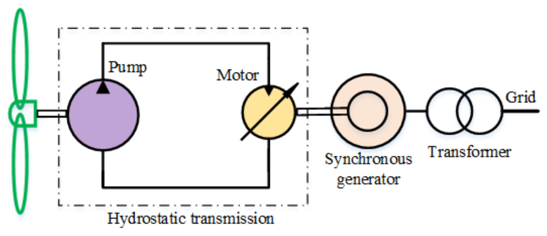The HST decouples the synchronous generator from the rotor speed, allowing it to operate at synchronous speed, eliminating the need for a power-electronics, substantially decreasing the cost of the drive train [9]. A schematic representation of the proposed HST drivetrain is shown in Figure 1.

Due to the compelling advantages of the HST wind turbine, the feasibility of using HST drive trains in utility-scale (>1 MW) turbines, has been extensively investigated [10,11]. Researchers at RWTH Aachen, have demonstrated a 1 MW turbine with multiple pumps and motors and a switching strategy to improve efficiency [12]. Simulation studies have been shown as an optimal control method to improve the power output of utility-scale HST wind turbines in low wind regimes [13]. Mitsubishi heavy industries and Artemis have developed 2.3 and 7 MW hydrostatic wind turbines with variable displacement and Digital Displacement Technology (DDT) pumps and motors [14,15]. Simulation studies demonstrate that digital hydrostatic drive trains can improve reliability and energy production [16]. Although these technologies show promising results in utility wind turbines, translating them to community wind turbines poses challenges in complexity, cost, and availability of the components.

In previous simulation work [9], we demonstrated the design and control of an HST wind turbine and the practicality of using an HST turbine with a synchronous generator coupled directly to the grid. In the current work, the behavior of an HST turbine under different wind disturbances is experimentally evaluated. For this study, a commonly available, single pump and motor configuration is used for the community wind as shown in Figure 1. An analytical model of the HST is developed and a pressure control framework to maximize the power capture is proposed. Hardware-in-the-loop (HIL) simulation is used to emulate the real wind turbine conditions on the power regenerative dynamometer to investigate the performance of the system. The performance of the turbine and controller is evaluated under transient and steady-state conditions. The efficiency of the transmission is measured and compared with the gearbox turbine.

To the best of our knowledge, this is the first time that a validated model and controlled experiments have been used to analyze the performance of this class of wind turbines. We suggest that understanding the dynamics and performance of the HST under varying wind conditions is critical to improving the performance of the components, fluids, and HST wind turbine.

Dynamical models for the HST and the control algorithm for a wind turbine are described in Section 2 and Section 3. The HIL experimental setup and the performance of the HST turbine subject to varying wind disturbances are discussed in Section 4 and Section 5. The performance of the HST is compared with a gearbox turbine in Section 6. Concluding remarks and future work are presented in Section 7.

2. Dynamic Model of the HST

In an HST, a pump drives a motor. With at least one variable displacement unit the system became a CVT. A fixed displacement pump and a variable displacement motor configuration are selected for the HST as shown in Figure 1. The turbine rotor rotates at a low speed, so a low-speed, high-displacement pump is required for the HST. Due to the unavailability of such pumps, a fixed-displacement, low-speed, and high-displacement hydraulic motor is used in reverse as a pump in our design. A variable-displacement, high-speed commercially available motor is selected to complement the pump. The rotor drives the hydraulic pump and produces a flow, Q, at pressure, $p_{\mathrm{t}}$. The dynamic equation for rotor speed, ${\omega }_{\mathrm{r}}$, is

$$\begin{array}{c}\hfill {\dot{\omega }}_{\mathrm{r}}=\frac{1}{J_{\mathrm{r}}}\left(-b_{\mathrm{r}}{\omega }_{\mathrm{r}}+{\tau }_{\mathrm{aero}}({\omega }_{\mathrm{r}},u_{\mathrm{w}},\theta )-p_t{D}_{\mathrm{p}}\right),\end{array}$$

(1)

where $J_{\mathrm{r}}$ and $b_{\mathrm{r}}$ are the inertia and viscous damping coefficient of the rotor. ${\tau }_{\mathrm{aero}}$, is the aerodynamic torque, which is a function of wind speed, $u_{\mathrm{w}}$, rotor speed, ${\omega }_{\mathrm{r}}$, and pitch angle of the blade, $\theta$. $D_{\mathrm{p}}$ is the pump displacement.

The pump flow is transmitted through a hydraulic line and drives the variable displacement motor. The short hydraulic line can be modeled as a fluid capacitance. The pressure in the control volume changes due to the difference between fluid entering and exiting the control volume. The dynamics of the line pressure, $p_{\mathrm{t}}$ is given by

$$\begin{array}{c}\hfill \dot{p_t}=\frac{B}{V}\left(D_{\mathrm{p}}{\omega }_{\mathrm{r}}-\alpha D_{\mathrm{m}}{\omega }_{\mathrm{g}}-L_{\mathrm{t}}{p}_{\mathrm{t}}\right),\end{array}$$

(2)

where V and B are the fluid volumes and bulk modulus. $D_{\mathrm{m}}$ is the full displacement of the motor and $\alpha$ is the normalized swash plate angle. The combined leakage loss from the hydraulic pump and motor, denoted by $L_{\mathrm{t}}$, is a linear function of the pressure and the leakage coefficient of the HST.

The hydraulic motor drives the synchronous generator and allows it to rotate at a constant speed. The motor swash plate angle is controlled by an electro-hydraulic valve. The dynamics of the swash plate position,$\alpha$, with respect to the applied voltage,$v_{\mathrm{t}}$ can be modeled as a first-order system. The gain and time constant are determined from the experiment and the transfer function is given by

$$\begin{array}{c}\hfill \alpha \left(s\right)=\frac{0.091}{0.3s+1}{v}_{\mathrm{t}}\left(s\right),v_{\mathrm{t}}\in [0,10]\end{array}$$

(3)

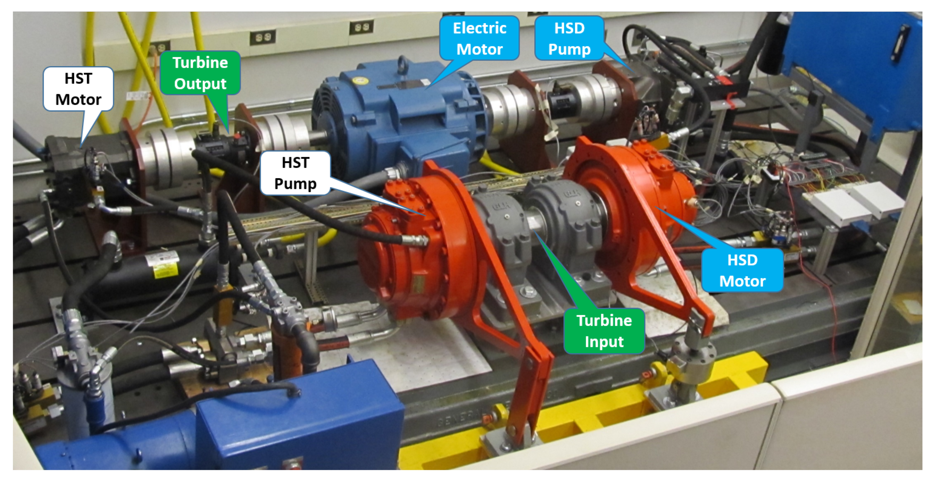
To measure the performance of the HST wind turbine, a $100\mathrm{kW}$ power regenerative wind turbine dynamometer has been developed at the University of Minnesota as shown in Figure 2 [17]. Unknown parameters in the HST dynamics equations are experimentally determined from the dynamometer and shown in

Table 1. HST parameters.

Description	Symbol	Value	Units
Viscous loss Coef.	$b_{\mathrm{r}}$	38.9	$\mathrm{Nm}/\sec$
Displacement of the pump	$D_{\mathrm{p}}$	$3.9980\times {10}^{-04}$	${\mathrm{m}}^3/\mathrm{rad}$
Displacement of the motor	$D_{\mathrm{m}}$	$2.1486\times {10}^{-05}$	${\mathrm{m}}^3/\mathrm{rad}$
Bulk Modulus	B	$1.8\times {10}^9$	Pa
Fluid Volume	V	$0.0018$	${\mathrm{m}}^3$
Leakage loss Coef.	$L_{\mathrm{t}}$	$5.0490\times {10}^{-12}$	${\mathrm{m}}^3/\sec .\mathrm{pa}$

[18].

3. HST Wind Turbine Control

Wind turbines operate in four control regions [19]. Our focus is in region 2, where the wind speed is between the cut-in speed and the rated speed and the control objective is the maximization of the power generation.

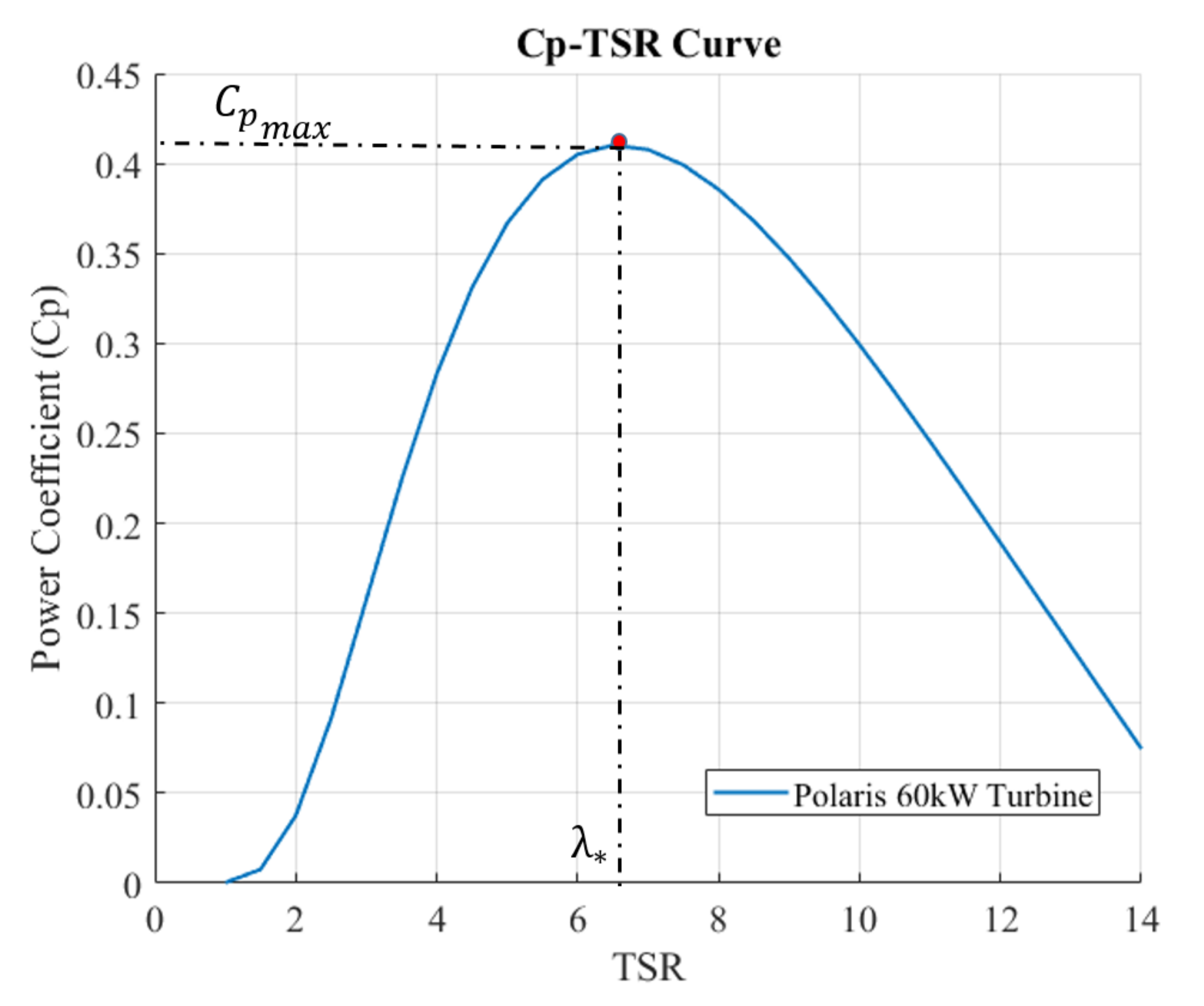
The aerodynamics efficiency of a wind turbine is measured by power coefficient, $C_{\mathrm{p}}$, the ratio between rotor power and wind power. $C_{\mathrm{p}}$ is a function of wind speed, $u_{\mathrm{w}}$, pitch angle and rotor speed, ${\omega }_{\mathrm{r}}$. According to Betz’s law, the maximum aerodynamic efficiency of a wind turbine rotor is $59\%$ [20,21]. In region 2, the blade pitch is fixed, and the control goal is to maximize the power capture. At a fixed pitch angle, the $C_{\mathrm{p}}$ of a turbine as a function of non-dimensional Tip Speed Ratio (TSR), $\lambda$. The TSR is defined as the ratio of tip speed velocity to wind speed:

$$\begin{array}{c}\hfill \lambda =\frac{{\omega }_{\mathrm{r}}R}{u_{\mathrm{w}}}.\end{array}$$

(4)

The desired maximum power coefficient, $C_{\mathrm{pmax}}$, is achieved by operating the turbine at the optimal TSR, ${\lambda }_{*}$, which is realized by controlling the rotor speed, ${\omega }_{\mathrm{r}}$.

$${\omega }_{\mathrm{r}}=\frac{D_{\mathrm{m}}{\omega }_{\mathrm{s}}}{D_{\mathrm{p}}}\alpha =\frac{{\lambda }_{*}{u}_{\mathrm{w}}}{R},$$

(5)

One approach, that might be used, is to control the rotor speed, ${\omega }_{\mathrm{r}}$, using the swash plate angle, $\alpha$, to operate the turbine at the optimal tip speed ratio [22]. However, this approach requires measuring wind speed, a difficult task in practice. Instead of controlling rotor speed directly, the load torque on the rotor shaft is controlled as described below.

In a conventional turbine, the load torque is computed by the $K{\omega }^2$ law and applied to the generator through power electronics. The controller always brings the turbine to the optimum point [23]. However, in the HST drive train, a synchronous generator is used and the rotor speed is controlled by the line pressure, $p_{\mathrm{t}}$, as shown in Equation (1).

In the hydraulic system, pressure is proportional to the torque. Neglecting the mechanical losses, the control pressure, $p_c$, is derived from the widely used torque control law.

$$p_{\mathrm{c}}=\frac{{\tau }_{\mathrm{c}}}{D_{\mathrm{p}}}=\frac{K{\omega }_{\mathrm{r}}^2}{D_{\mathrm{p}}}$$

(6)

where K is given by

$$K=\frac{1}{2}\rho A{R}^3\frac{C_{\mathrm{pmax}}}{{\lambda }_{*}^3}$$

(7)

where $\rho$, A, and R are the air density, rotor swept area, and distance from the rotor center to the tips of the blade, respectively. $C_{\mathrm{pmax}}$ is the maximum power coefficient and ${\lambda }_{*}$ is the optimal TSR.

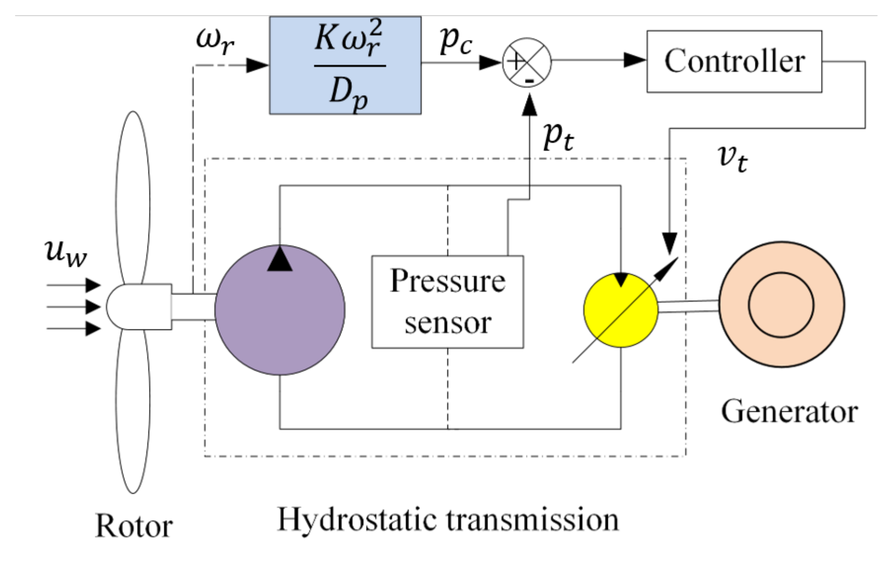
The HST pressure is electronically controlled by the HST motor swash plate voltage. The system has two states and one actuator dynamics. The transfer function from voltage input, $v_{\mathrm{t}}$ to the pressure, $p_{\mathrm{t}}$ is a third-order system. To minimize the tracking error and reject disturbances, a PI controller is implemented to determine the swash plate voltage [9,24]. The control schematic is shown in Figure 3. The performance of the HST and controller is measured on the power regenerative dynamometer.

To implement the pressure controller, we only need the rotor speed for the reference command and the pressure for tracking. The pressure control automatically brings the turbine to the optimum point, since the reference command includes optimal values of ${\lambda }_{*}$ and $C_{\mathrm{pmax}}$. With knowledge of accurate turbine parameters, the pressure control method can maximize the power capture without measuring the wind speed.

4. Experimental Setup

Performance validation of the designed HST drive train in a commercial wind turbine is a daunting task. The wind turbine requires modification to accommodate the HST drive train in its nacelle. Real-time diagnosis on the tall tower is also challenging.

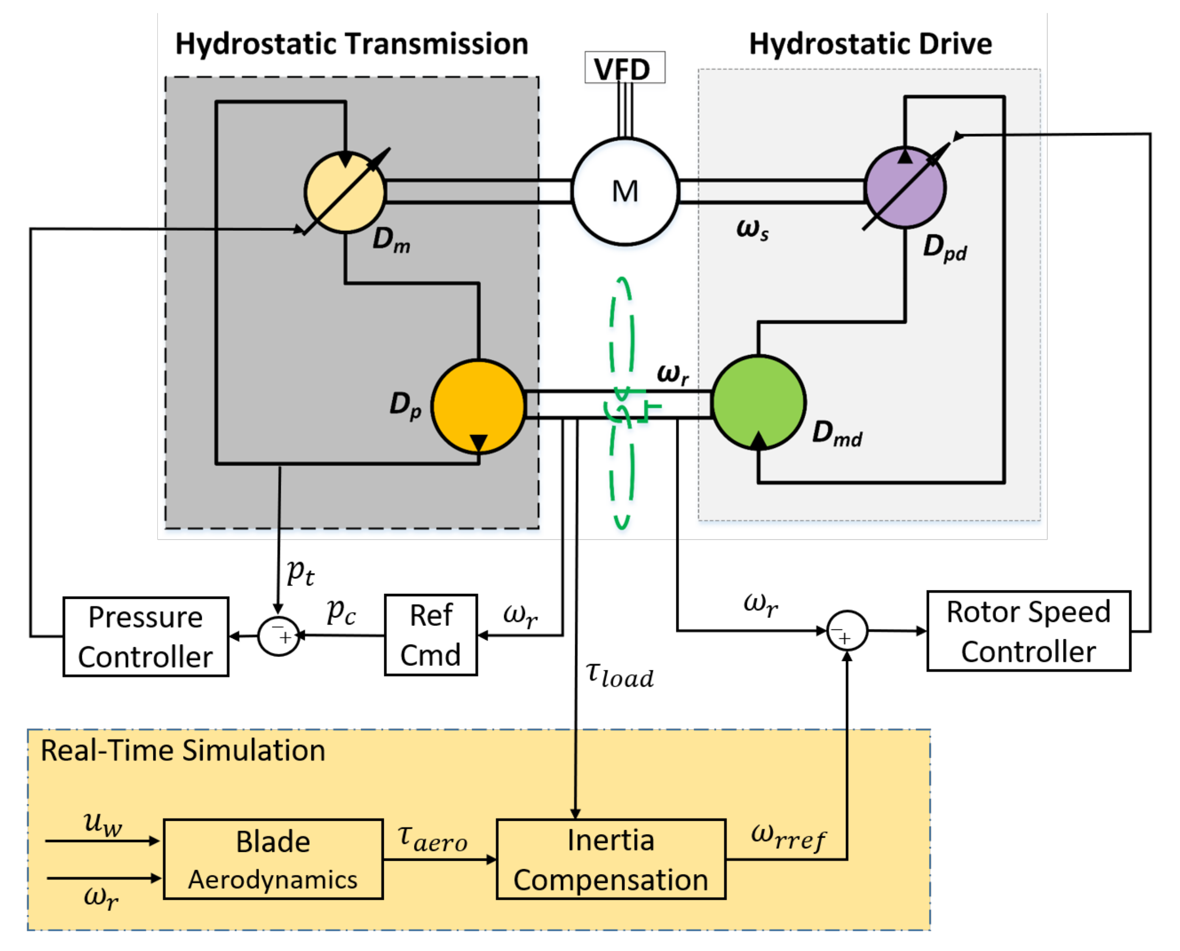
Hardware-in-the-loop (HIL) simulation is developed to validate the performance of the HST drive train and its control strategy, in a virtual wind turbine environment before implementation on a wind turbine system. The HIL test architecture on the power regenerative research platform is illustrated in Figure 4. The real-time aerodynamic torque, ${\tau }_{\mathrm{aero}}$ in the HIL simulation, is determined by a look-up table using wind data and rotor speed.

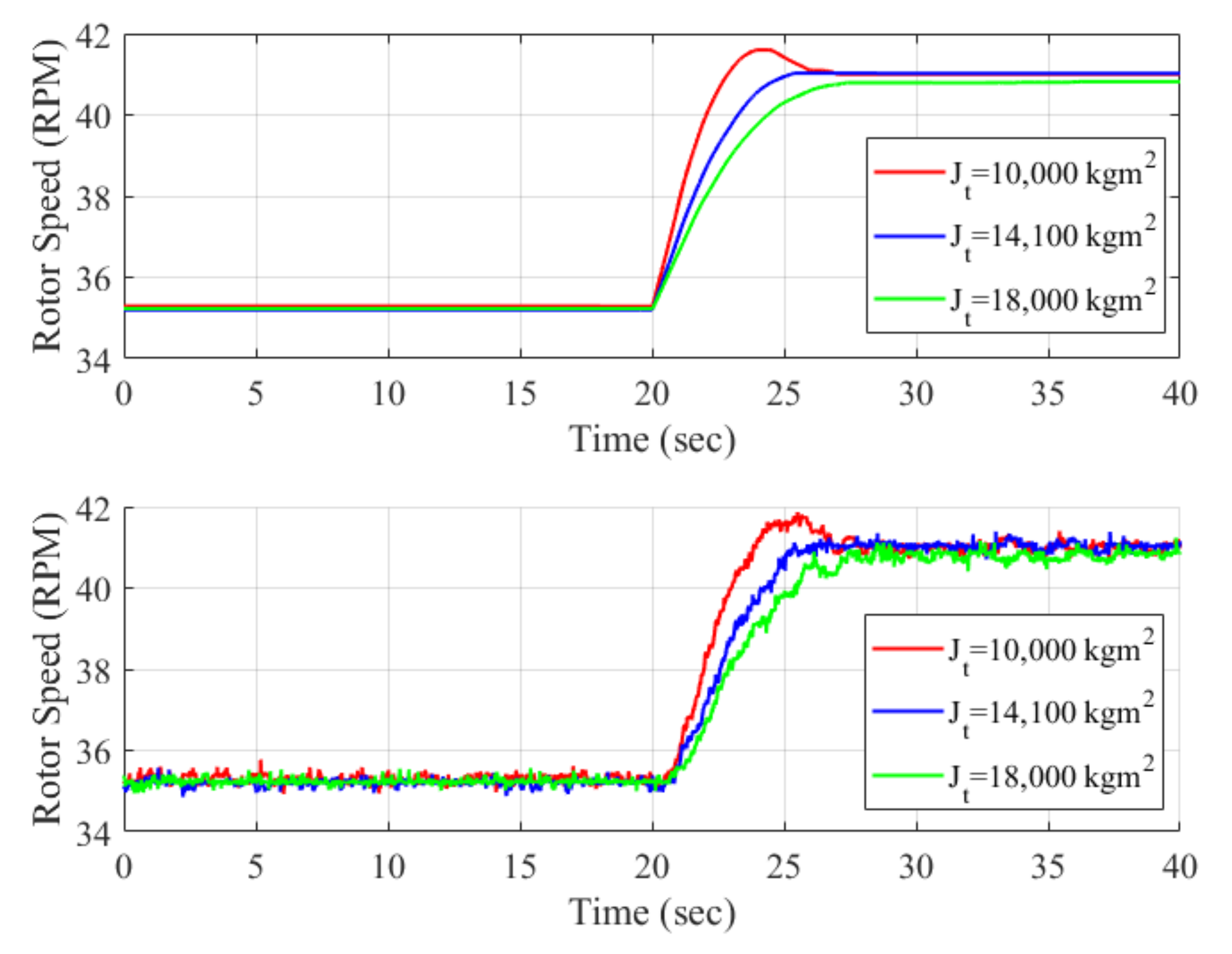
The inertia of the turbine rotor, $J_{\mathrm{t}}$ has a considerable effect on the dynamic behavior of the turbine. It is not feasible to install a large flywheel on the dynamometer. As a result, the rotor on the dynamometer has significantly lower inertia than that of a real turbine. To simulate the dynamics of a turbine rotor, it is necessary to consider the effect of large blade inertia in a real-time simulation. The measured load torque on the rotor shaft of the dynamometer, ${\tau }_{\mathrm{load}}$, is fed to the simulation. The reference rotor speed ${\omega }_{{\mathrm{r}}_{\mathrm{ref}}}$ is computed from ${\tau }_{\mathrm{load}}$, ${\tau }_{\mathrm{aero}}$, and turbine rotor inertia using Equation (8). The computed speed is sent to the dynamometer and emulated by controlling the swash plate of the HSD pump. The rotor speed is tracked by implementing a feedback controller.

$${\omega }_{{}_{{\dot{\mathrm{r}}}_{\mathrm{ref}}}}=\frac{1}{J_{\mathrm{t}}}({\tau }_{\mathrm{aero}}-{\tau }_{\mathrm{load}});{\tau }_{\mathrm{load}}=D_{\mathrm{p}}{p}_{\mathrm{t}}$$

(8)

The HST motor swash plate is controlled to achieve maximum power in the turbine. Power from the drivetrain is fed to the dynamometer to assist the electric motor to drive the HSD pump.

Electric grid transients can be simulated in a HIL simulation. The dynamometer is capable of emulating the grid frequency in the high-speed shaft using the electric motor and VFD controller. The detailed dynamics and control of the power regenerative dynamometer are described in Mohanty et al. [24].

The dynamometer is equipped with a pressure, flow, and temperature sensor in all fluid lines, and torque and speed sensor in all mechanical lines. The sensors are calibrated per industrial standards. The overall uncertainty of each sensor is less than $1.5\%$. The sensor data are collected by NI-DAQ at a 1 kHz sampling frequency. Matlab Simulink Real-Time is used for real-time data acquisition and dynamometer control.

4.1. Test Turbine

In this paper, the performance of the HST is investigated for a 60 kW, horizontal axis, and variable speed turbine, manufactured by Polaris America (www.polarisamerica.com, accessed on 13 November 2021). The speed and torque range of the selected turbine is within the operating range of the HST wind turbine transmission in our dynamometer. No such turbines with complete specifications are available. All needed turbine parameters are available, except the $C_{\mathrm{p}}$ curve and rotor inertia. The parameters of the turbine are listed in

Table 2. Test turbine data and its comparison with an NREL turbine.

Specification	Symbol	Reference Turbine	Test Turbine
Turbine Model		AOC 15/50	P21-60
Rated Power	P	50 kW	60 kW
Number of Blades		3	3
Rotor Radius	R	7.5 m	10.6 m
Hub Height	H	25 m	30 m
Rotor Inertia	$J_{\mathrm{t}}$	$5000\mathrm{kg}{\mathrm{m}}^2$	14,100 $\mathrm{kg}{\mathrm{m}}^2$
Rated Wind Speed	$u_{\mathrm{wr}}$	11 m/s	10 m/s
Max Rotational Speed	$W_{\mathrm{rmax}}$	65 RPM	58 RPM
Power Coefficient	$C_{\mathrm{pmax}}$	0.4512	0.41
Optimal TSR	${\lambda }_{\mathrm{opt}}$	6.545	6.5

. The $C_{\mathrm{p}}$ curve is generated by the standard mathematical equation as shown in the section below. The rotor inertia is computed by scaling the rotor inertia of the NREL AOC 50 kW reference turbine, creating the best available model for a 60 kW turbine.

4.2. Rotor Aerodynamics

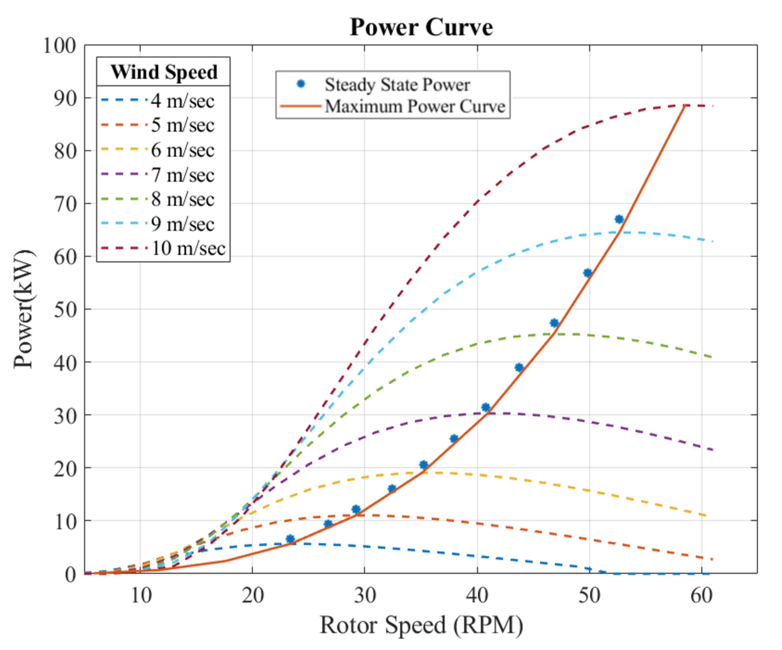
An important parameter for power regulation is the power coefficient, $C_{\mathrm{p}}$, of the turbine. It is a nonlinear function and depends on the blade design. The $C_{\mathrm{p}}$ values of the test turbine are not disclosed by the manufacturer, and thus, had to be derived analytically. The $C_{\mathrm{p}}$ as a function of the tip speed ratio and the blade pitch angle, $\theta$ is shown in Equation (9) [25,26].

$$\begin{array}{c}\hfill C_{\mathrm{p}}(\lambda ,\theta )=c_1(\frac{c_2}{{\lambda }_{\mathrm{i}}}-c_3\theta -c_4{\theta }^x-c_5)e^{-\frac{c_6}{{\lambda }_{\mathrm{i}}}},\\ \hfill \frac{1}{{\lambda }_{\mathrm{i}}}=\frac{1}{\lambda +0.08\theta }-\frac{0.035}{{\theta }^3+1}\end{array}$$

(9)

where the values of the coefficients $c_{\mathrm{i}}$ for $i\in [1,6]$ and x depend on the turbine type. The maximum power coefficient, $C_{\mathrm{pmax}}$, is computed from the output power curve data, assuming the drive train efficiency of $90\%$. The $C_{\mathrm{p}}$ of the test turbine for $\theta =0$ and $c=[0.1564;116;0.4;0;3.5;11.5]$ is plotted in Figure 5.

The value of ${\lambda }_{*}$ of the test turbine is determined from the $C_{\mathrm{p}}$ curve and implemented in the controller design. Using the non-dimensional $C_{\mathrm{p}}$-TSR curve, the aerodynamic torque of the rotor, ${\tau }_{\mathrm{aero}}$, is derived as a function of the rotor speed and wind speed. The look-up table of the aerodynamic torque is implemented in the HIL simulation.

4.3. Rotor Inertia

The rotor inertia of the test turbine is derived from the reference turbine. The moment of inertia of a blade about the rotor axis is given as

$$I_{\mathrm{r}}=\frac{1}{3}M{L}^2=\frac{1}{3}{\rho }_{\mathrm{b}}{A}_{\mathrm{b}}{L}^3\propto A_{\mathrm{b}}{L}^3$$

(10)

where M and L are the mass and length of a turbine blade. The mass is proportional to the density, ${\rho }_{\mathrm{b}}$, cross-sectional area, $A_{\mathrm{b}}$ and length. If the blade cross-sectional area and material density of the test turbine are assumed to be equal to that of the reference turbine, the moment of inertia is proportional to the third power of the blade length. Thus the rotor inertia is scaled with respect to that of the reference turbine.

4.4. Wind Input

The average wind speed varies greatly on a seasonal, hourly, and short-term basis, due to the effects of air density, altitude, surface topology, etc. Daily variations in solar radiation cause diurnal fluctuations. Short-term wind speed variation is manifested as wind turbulence and gusts.

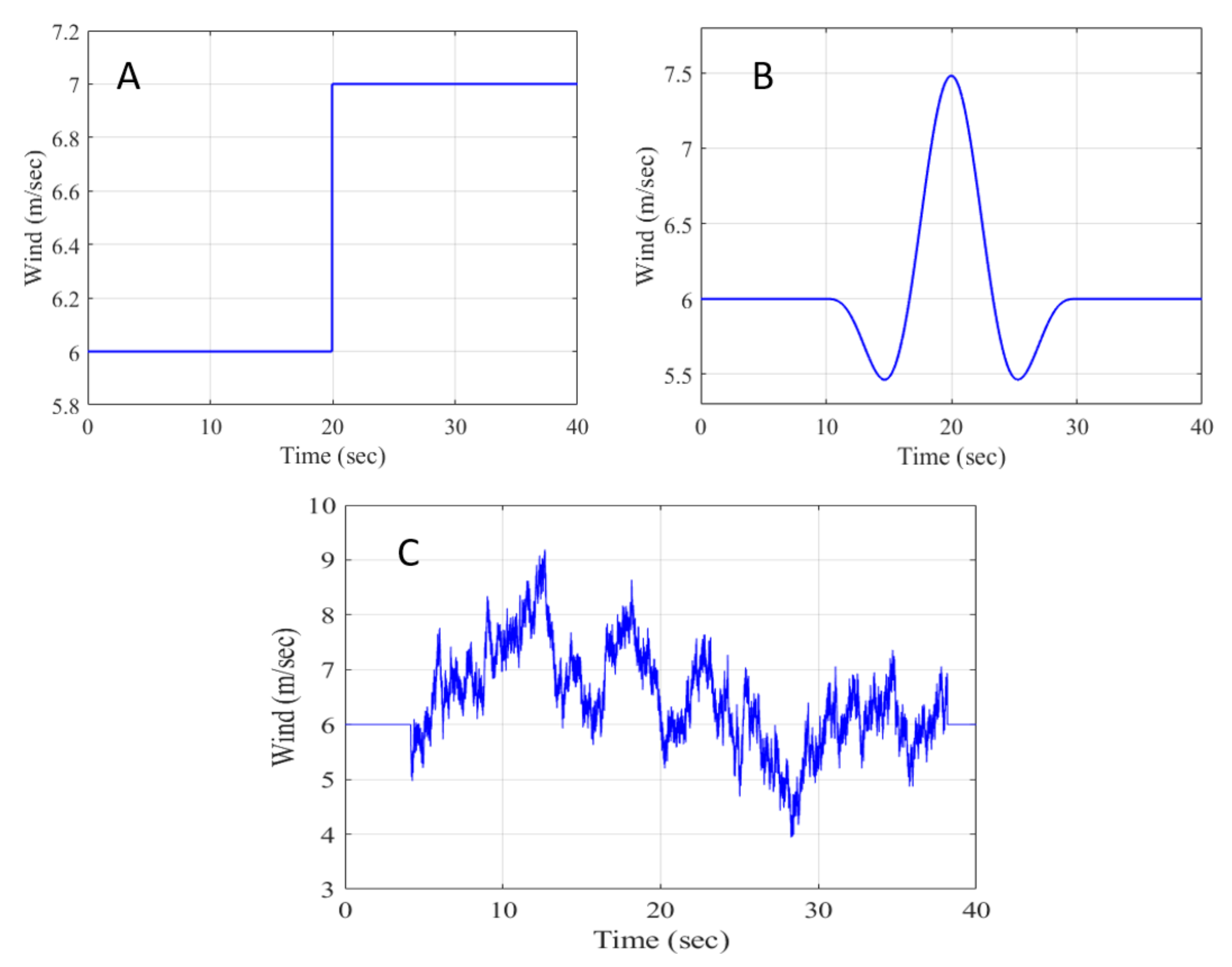
The HST wind turbine performance is measured under three wind profiles: (i) a step input, (ii) a wind gust, and (iii) turbulent wind.

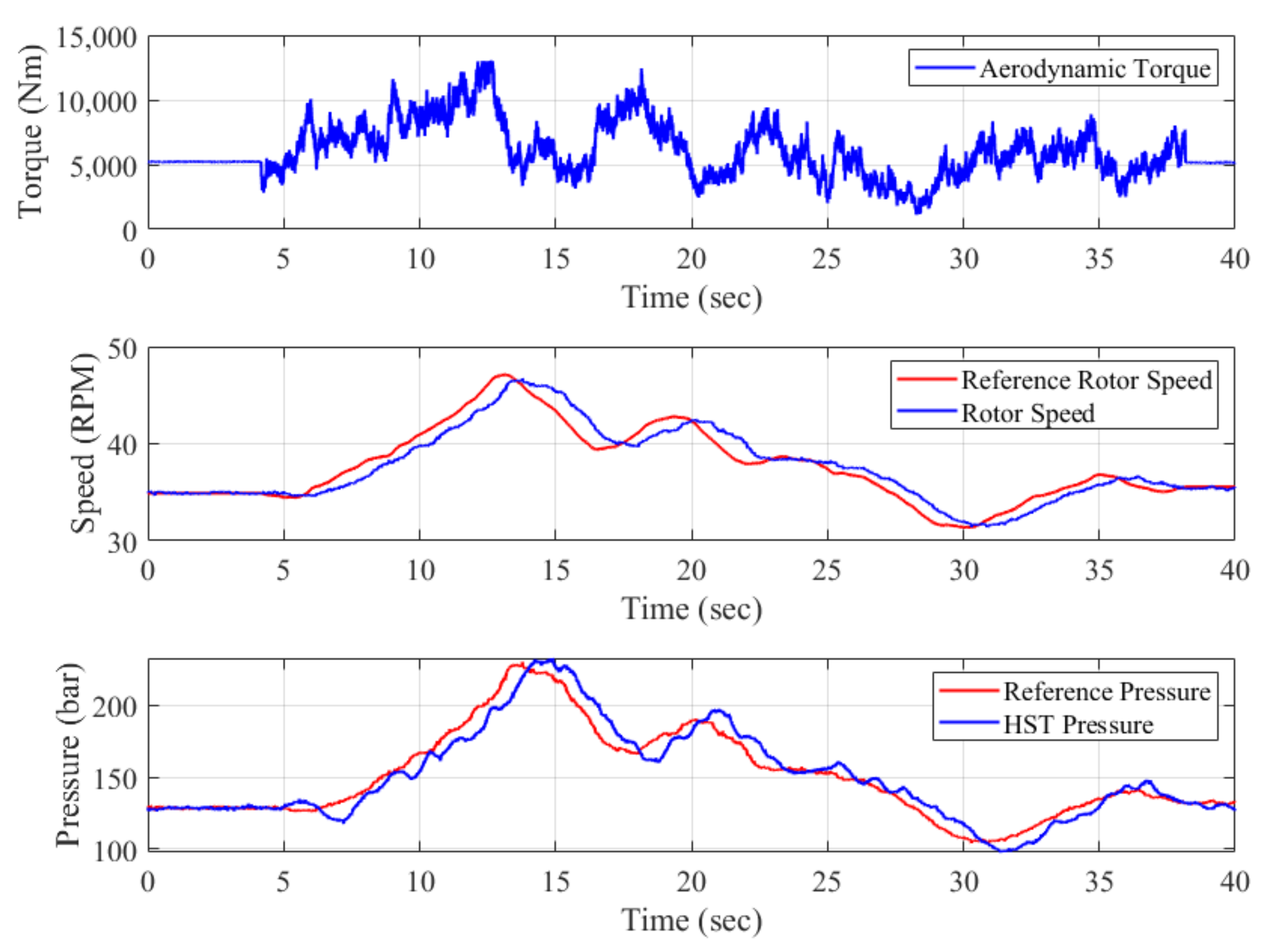
During the step input, the wind speed is changed from $6\mathrm{m}/\mathrm{s}$ to $7\mathrm{m}/\mathrm{s}$ at the 20 s time point, shown in Figure 6A. The gust wind profile, shown in Figure 6B, is created according to the IEC standard [27]. The turbulent wind profile, shown in Figure 6C, is created using Turbsim, a stochastic, turbulent wind simulator developed by NREL [28]. The hub height wind speed is computed using the IEC Kaimal spectral model with a mean turbulence intensity of $16\%$ at $15\mathrm{m}/\mathrm{s}$.

5. Results

The operation of the HST drive train has been tested in different wind conditions. The results of steady and dynamic conditions are discussed below. To maximize the operating range of the HST motor swash plate, the high-speed shaft speed is set to 1200 RPM.

5.1. Dynamic Behaviour

The dynamic behavior of the HST wind turbine is measured under three distinct wind conditions. The HST pressure is controlled to optimize the power as discussed in Section 3.

Step Wind: The responses to step wind are shown in Figure 7. It can be seen that the step rise in wind exerts a steep increase in the torque which subsequently leads to an increase in rotor speed. The torque gradually decreases due to the increase in the rotor speed. The reference rotor speed, generated by the HIL simulator and the measured speed, is shown in the second plot. The rotor controller tracks the reference. Although the controller has a bandwidth of 3 rad/s, the inertia of the rotor dominates and it takes significantly longer to reach the final value.

The reference pressure, computed from the rotor speed and the measured HST pressure are shown in the third plot. The measured HST pressure tracks the reference pressure with a small delay.

Gust Wind: The aerodynamic torque applied to the rotor during a wind gust is shown in the first plot of Figure 8. It can be seen that the torque and rotor speed follow the same trend as the wind profile. The corresponding reference rotor speed and the rotor speed of the dynamometer are illustrated in the second plot. Due to the large inertia, the reference speed has a delay from the torque input. The measured HST pressure along with their reference signals are shown in the third plot. Both of the measured signals effectively track their reference counterparts, with a delay.

Turbulent Wind: The torque on the rotor during turbulent wind is shown in Figure 9. The torque has high-frequency content from the wind. However, the large inertia of the rotor filters out most of the high-frequency content of the turbulent wind. The smooth profile of the reference rotor speed and the measured rotor speed is illustrated in the second plot. In the third plot, the turbine controller effectively tracks the reference signal to operate the turbine near-optimal tip speed ratio.

5.2. Effect of Inertia

The effect of inertia on the rotor speed is evaluated on the dynamometer by comparing three sampled values for inertia. The results of the HIL simulation and the measured rotor speed are illustrated in Figure 10. The response time varies with the rotor inertia, with the smallest inertia showing the smallest response time. The implemented controller accurately tracks the desired rotor speed.

5.3. Steady-State Analysis

For steady-state performance, the wind speed is increased from 4 m/s to 9 m/s in steps of 0.5 m/s. The rotor power is computed from the input torque and the rotor speed. The simulated power as a function of the wind and rotor speed and the maximum power curve is shown in Figure 11. The steady-state power measurements are also plotted.

The steady-state measurements at each wind speed follow the maximum power curve. The measured power is slightly higher than the simulated power because of the viscous loss in the rotor shaft.

5.4. Efficiency

The overall efficiency, $\eta$, of the HST transmission is computed with ISO 68 hydraulic oil in the operating wind regime. The $\eta$ is defined as the ratio between HST motor output power and rotor power.

$$\eta =\frac{P_{\mathrm{HST}}}{P_{\mathrm{rot}}}=\frac{{\tau }_{\mathrm{t}}{\omega }_{\mathrm{s}}}{{\tau }_{\mathrm{r}}{\omega }_{\mathrm{r}}}$$

(11)

The HST power is a product of the HST motor torque, ${\tau }_{\mathrm{t}}$, and speed, ${\omega }_{\mathrm{s}}$, whereas the rotor power, is a product of applied rotor torque, ${\tau }_{\mathrm{r}}$, and speed, ${\omega }_{\mathrm{r}}$. The efficiency as a function of the wind speed is shown in the top plot of Figure 12. The HST pressure and the motor swash plate voltage are plotted in the middle plot.

The measured overall efficiency is $80\%$ for the wind speeds above $7\mathrm{m}/\mathrm{s}$. With decreasing wind speed, the efficiency gradually declines due to low operating pressure and swash plate position. Wind power varies as the cube of the wind speed. As shown in Figure 11, at low wind speeds the power is less significant.

The overall efficiency of the transmission is less than expected. To understand these losses, the efficiency of the individual components is plotted in the bottom plot. The overall efficiency is a product of the efficiency of the hydraulic pump, ${\eta }_{\mathrm{p}}$ and motor, ${\eta }_{\mathrm{m}}$.

$$\eta ={\eta }_m{\eta }_p=\frac{P_{\mathrm{HST}}}{P_{\mathrm{fluid}}}*\frac{P_{\mathrm{fluid}}}{P_{\mathrm{rot}}}$$

(12)

The power in the fluid, $P_{\mathrm{fluid}}$, is the product of pressure difference in the hydraulic line, p, and flow in the hydraulic line, Q. From the bottom plot of Figure 12, it can be seen that the fixed displacement pump operated at a 95% efficiency and had negligible changes with respect to the decreasing wind speed. In contrast, the variable displacement hydraulic motor operated at 85% efficiency, which is less than the manufacturer efficiency tested with ISO-32 hydraulic oil. One of the reasons is that the hydraulic motor is designed for high-speed operation and performs well with low-viscosity oil. The efficiency of the system can be raised to 86–88% by substituting it with a lower viscosity oil. This is likely to enhance the efficiency of the HST pump by 1–2% in high-speed operations as well as that of the HST motor by 6–7%. The efficiency in the low-wind regime could be improved by using a more efficient variable displacement motor such as a digital displacement motor [29] or linkage motor [30].

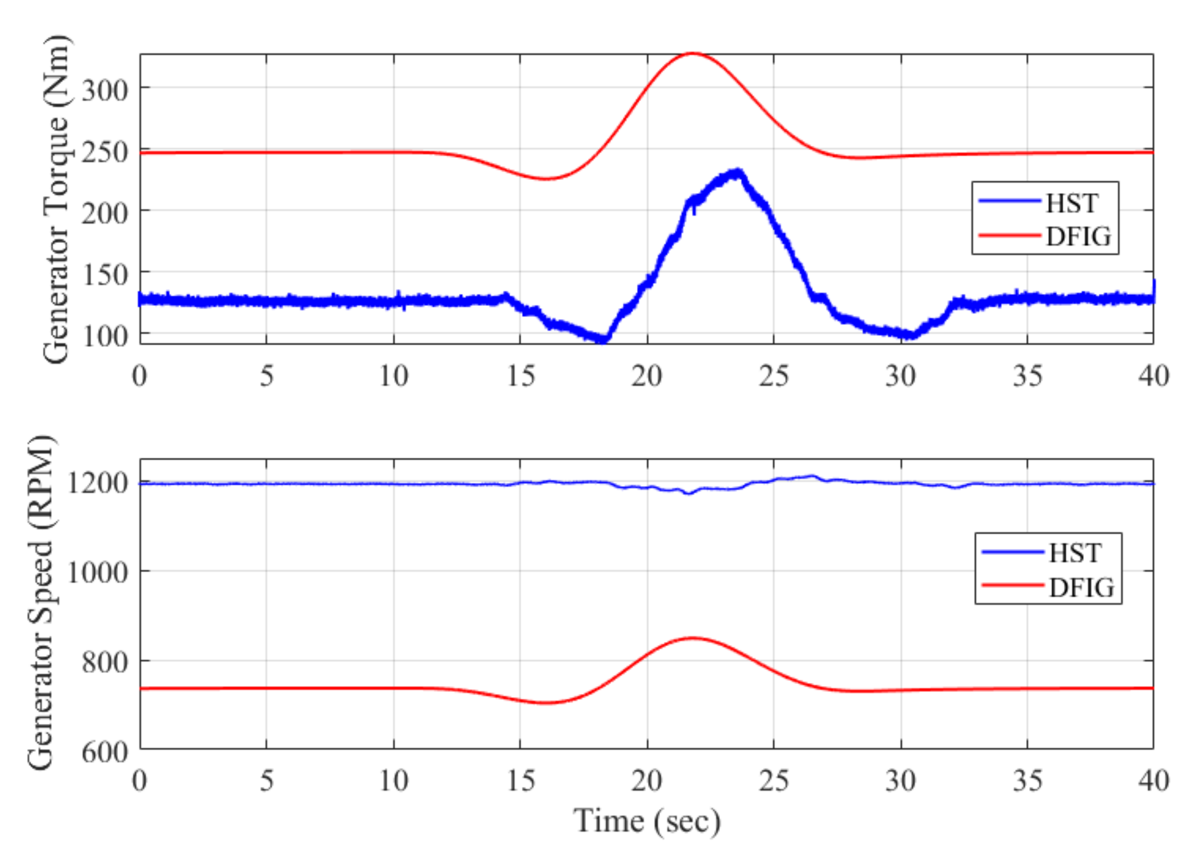
6. Comparisons

The performance of the HST drive train is compared with a simulated 60 kW gearbox turbine (GB). The gearbox turbine is equipped with the same rotor, but the drive train contains a gearbox, an induction generator, and power electronics. For the simulation, a gear ratio of 21 is selected to match the generator speed of $1200\mathrm{RPM}$ at the rated rotor speed. Figure 13 shows the torque and speed of both the HST drive train and simulated gearbox drive train in response to the wind gust in Figure 6.

From Figure 13, the torque on the generator shaft is lower in the HST turbine than in the gearbox turbine, but the generator speed is higher in the HST turbine. When the input wind speed is less than rated, in the case of a gearbox turbine, the generator speed is less than the synchronous speed. As the generator speed in the gearbox turbine fluctuates in the face of a wind gust, power electronics are required to match the grid frequency. In the HST drive train, the generator speed remains nearly constant at synchronous speed despite the wind gust. The HST decouples the generator speed from the rotor speed allowing the generator to rotate at synchronous speed.

Table 3. Comparison between an HST and a gearbox wind turbine.

Components	Weight (kg)		Cost (%)		Efficiency (%)
	GB	HST	GB	HST	GB	HST
Transmission	820	400	13	10	95	86
Generator	-	-	3.5	3.5	96	98
Power Electronics	-	-	5	0	95	-
Total	820	400	21.5	13.5	87	84

compares the weight, cost, and efficiency of an HST and a gearbox turbine. The weight comparison is based on a 100 kW turbine. The HST weight includes the HST pump, motor, and hydraulic ancillaries and the gearbox weight includes the Flender gearbox and gear oil [31]. The weight of the synchronous generator and induction generator is assumed to be the same and the weight of the power electronics in the gearbox turbine is neglected. The HST drive train is 50% lighter than the gearbox drive train.

In a gearbox turbine, the drive train is capital intensive. The cost of the gearbox is 13%, the generator is 3.5%, and the power electronics is 5% of the total turbine cost [32]. Gearboxes for wind turbines are expensive because of their high torque capacity. However, HSTs are highly suitable for this high torque application. Industrial products in this power range are readily available, limiting the HST cost to 10% of the turbine cost. The HST wind turbine does not require power electronics, resulting in a total cost saving of 8%.

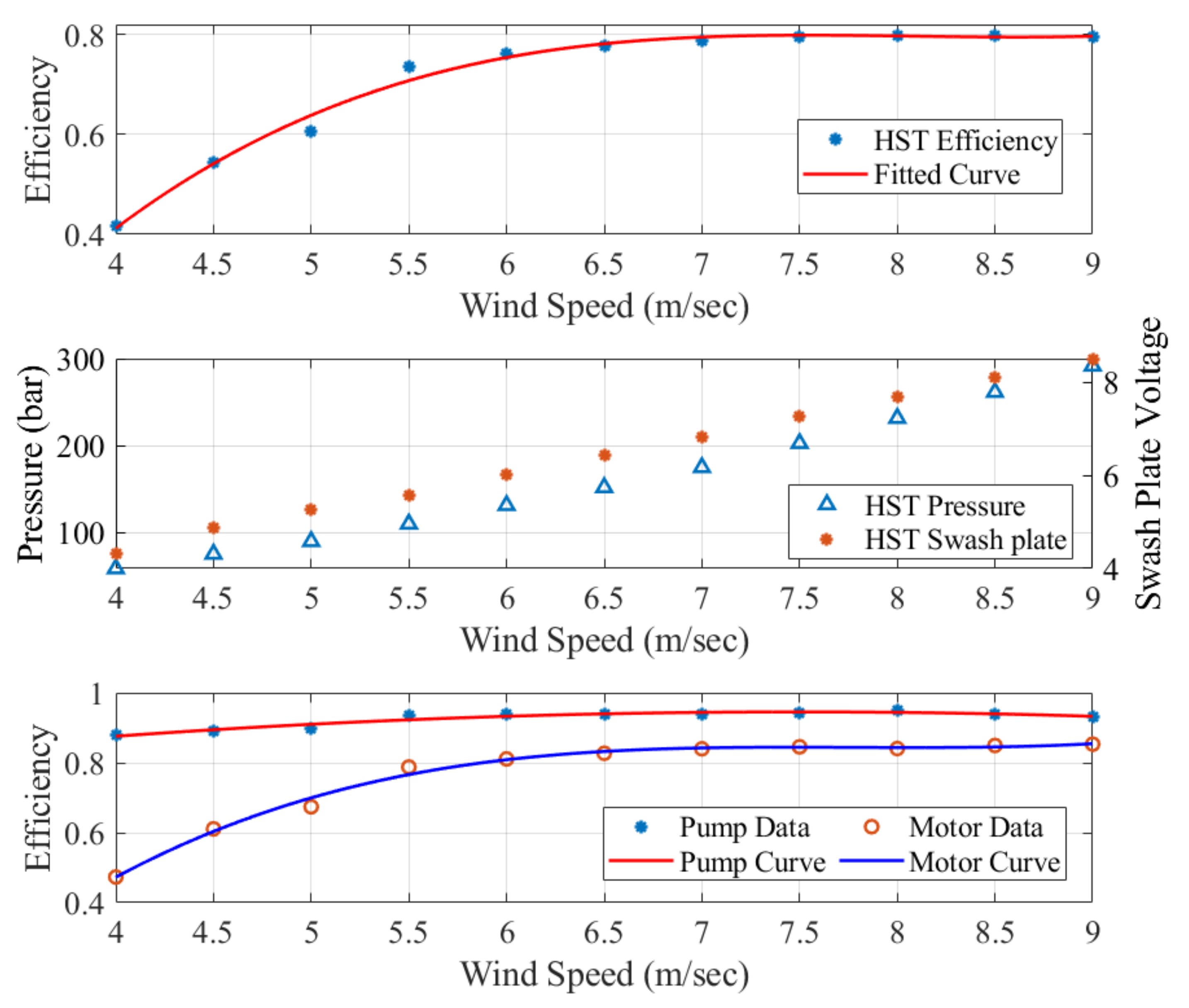
The power efficiency of the HST wind turbine is also compared with a gearbox turbine in Table 3. For the analysis, the power loss in a gearbox, induction generator, and power electronics is assumed to be 5%, 4%, and 5%, respectively [33]. As discussed in the previous section, reasonable values for the HST efficiency would be 86%, and for the synchronous generator would be 98%. Even though the HST efficiency is less than the gearbox efficiency the overall system efficiencies are comparable. This means the Levelized cost of electricity (LCOE) would be lower for the HST wind turbine.

7. Conclusions

A hydrostatic transmission is a cheaper, lighter, and more reliable alternative for a community wind turbine. Dynamic equations of the HST and corresponding pressure control strategy are developed. The HIL simulation allows us to test the HST drive train on the power regenerative dynamometer under virtual wind conditions. The pressure controller demonstrates good tracking performance to optimize the power during the step, turbulent, and gust wind inputs. Although the controller has a high bandwidth, the large inertia of the rotor dominates and slows down the control response. The proposed approach controls the rotor speed so that the turbine is near the optimal tip-speed ratio to maximize the power capture. The HST decouples the generator speed from the rotor speed allowing the generator to rotate at synchronous speed. The hydrostatic transmission can be an attractive alternative for a variable-speed wind turbine without power electronics. Our next goal is to further improve the performance of the HST turbine by developing advanced control strategies, hybridizing the transmission with a hydraulic accumulator, and using more efficient components and fluids.