Extending DC Bus Utilization for Induction Motors with Stator Flux Oriented Direct Torque Control

Abstract

This paper presents a method to extend the DC bus utilization on an induction motor (IM) by using a combination of Space-Vector Modulated Direct Torque Control (DTC–SVM) and conventional DTC. The scheme proposed in this paper exploits the advantages of both control methods. During the linear region, it allows for a low torque ripple and low current harmonic distortion (THD). During the overmodulation region, it allows for the fastest torque response up to the six-step operation region. In both regions, there is complete independence of the motor parameters. The paper describes a way to provide a smooth transition between the two control schemes. Non-linearities affect the stator flux angle estimation, which leads to the inability to decouple torque and flux. To overcome this problem, a novel PI-based control scheme as well as a simplification on the decoupling terms’ calculation are proposed. Simulation and experimental results are presented to verify the feasibility of the proposed method.

1. Introduction

The increased global demand for energy, along with the diminishing stocks of the most traditional fossil fuels, have accelerated the transition to cleaner, more efficient energy sources [1,2]. Transportation has been highly influenced by these circumstances, causing the number of battery-powered vehicles to grow rapidly, as well as the number of researchers who have focused on this issue [3,4]. Due to the relatively low operation voltage of electric vehicle (EV) batteries, one of the most important aspects for an EV is to maximize the usage of the voltage provided by its batteries. Among other reasons, since the fundamental amplitude of the maximum output voltage for Space Vector Pulse Width Modulation (SVPWM) is around 15.5% greater than for Sinusoidal Pulse Width Modulation (SPWM), SVPWM is extensively implemented [5,6,7,8,9,10,11,12]. However, even though the DC bus voltage utilization during the linear region is greater than for SPWM, it is still limited to the 90.7% of the DC bus capability, leaving some of the DC bus voltage to be unusable [13,14,15,16].

With the growing demand for acceleration and torque of electric cars, all for a battery-powered low-voltage inverter, more researchers have focused on implementing SVPWM strategies in the overmodulation region. These strategies are commonly classified into two groups. The first group is composed by overmodulation strategies that only have one operation region [17,18,19,20]. On the other hand, the second group is formed by strategies which have two operation regions [20,21,22,23,24,25,26,27,28]. In [17], the single-region approach was implemented. However, this control method has the disadvantages of phase angle mutation, low control accuracy and output discontinuity. To improve the control accuracy, a standardized dual-region overmodulation approach was proposed in [27]. In this strategy, the division of the two regions is based on the modulation index. Nevertheless, this approach requires offline calculations and high computing power. Aiming to overcome these drawbacks, a piece-wise fitting linear analysis was proposed in [28]. Nonetheless, this approach requires simultaneous correction of the module and phase angle of the reference voltage vector. Hence, it has the disadvantages of the necessity to include two modification algorithms and high computational complexity. Another strategy based on the superposition principle to eliminate the tedious off-line calculations and look-up routines was proposed in [29,30]. However, although the off-line computation has been eliminated, high computational cost and two modification algorithms are required. Furthermore, all the overmodulation strategies described above suffer from deterioration of current control performance due to voltage saturation, which is a result of the limited available voltage to offset the back electromotive force (EMF) [31]. Moreover, the increase of current harmonic content degrades the controllability of these PI controller-based systems, resulting in poor transient behavior and, in the worst case, total system uncontrollability [32,33,34]. The literature [35] presented an additional method to filter the current harmonics to improve control performance. Such method, however, also reduce the current loop bandwidth, resulting in a slow transient response within the overmodulation region. The comparison of state-of-the-art methods is summarized in

Table 1. Comparison of state-of-the-art methods.

Overmodulation Strategy	Advantages	Disadvantages
Single mode [17]	Simple algorithm.	Phase angle mutation, low control accuracy, output discontinuity.
Dual mode [27]	Good control accuracy.	Computational complexity, offline data computing.
Piecewise fitting [28]	No need for offline data computing and look-up process.	Two modification algorithms, high computational complexity, simultaneous correction of amplitude and phase angle of the reference voltage vector.
Superposition principle [29,30]	No need for offline data computing and look-up process.	Two modification algorithms, high computational complexity.

.

This paper addresses the problems of complexity and degraded controllability of state-of-the-art overmodulation methods, as well as the problem of motor parameter dependency. The scheme presented in this paper is based on the combination of conventional DTC [36] and DTC–SVM [37] to exploit their respective advantages. A simple, yet effective algorithm is proposed to ensure a smooth transition between the two control modes. Additionally, a simplified method to decouple torque and flux is developed. Finally, a compensation of the nonlinearities which deteriorate the stator flux angle estimation is also proposed in this paper.

The control algorithm presented in this paper has the following advantageous attributes:

• Independence of motor parameters and, hence, robust control throughout the whole operation region.
• Maximum utilization of the DC bus capability.
• Maximum operating range of the constant torque region.
• Accurate torque and flux decoupling.
• Accurate stator flux calculation.
• Smooth transition between control modes.
• Instantaneous torque response during the overmodulation region.
• Low computational cost.
• Robust slip speed estimation without differentiation of the q-axis component of the stator current $\left({\mathrm{i}}_{\mathrm{qs}}\right)$.

Finally, simulation and experimental measurements were performed on a 1.5 kW IM inverter system to verify the feasibility of the proposed method.

2. Conventional DTC Principles

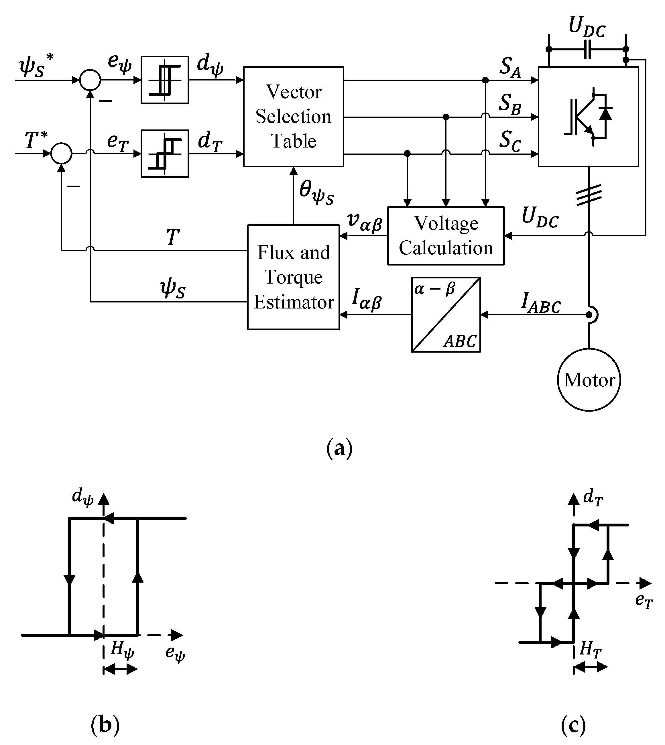
The conventional DTC scheme proposed by Takahashi [36] has the following working principle, as shown in Figure 1a. The error between the estimated torque $\left(\mathrm{T}\right)$ and the reference torque $\left({ \mathrm{T}}^{*}\right)$ is the input of the three-level hysteresis comparator that can be found in Figure 1b. Similarly, the error between the estimated stator flux magnitude $\left({\mathsf{\psi }}_{\mathrm{s}}\right)$ and the reference stator flux magnitude $\left({\mathsf{\psi }}_{\mathrm{s}}{}^{*}\right)$ is the input of the two-level hysteresis comparator that can be found in Figure 1c.

The digitized output of the flux and torque hysteretic controllers, as well as the stator flux position sector are the inputs to select the appropriate voltage vector from the switching table, which can be found in

Table 2. Conventional DTC optimum switching table.

${\mathbf{d}}_{\mathsf{\psi }}$	$d_T$	Sector 1	Sector 2	Sector 3	Sector 4	Sector 5	Sector 6
1	1	${\mathrm{U}}_2$	${\mathrm{U}}_3$	${\mathrm{U}}_4$	${\mathrm{U}}_5$	${\mathrm{U}}_6$	${\mathrm{U}}_1$
	0	${\mathrm{U}}_7$	${\mathrm{U}}_0$	${\mathrm{U}}_7$	${\mathrm{U}}_0$	${\mathrm{U}}_7$	${\mathrm{U}}_0$
	−1	${\mathrm{U}}_6$	${\mathrm{U}}_1$	${\mathrm{U}}_2$	${\mathrm{U}}_3$	${\mathrm{U}}_4$	${\mathrm{U}}_5$
0	1	${\mathrm{U}}_3$	${\mathrm{U}}_4$	${\mathrm{U}}_5$	${\mathrm{U}}_6$	${\mathrm{U}}_1$	${\mathrm{U}}_2$
	0	${\mathrm{U}}_0$	${\mathrm{U}}_7$	${\mathrm{U}}_0$	${\mathrm{U}}_7$	${\mathrm{U}}_0$	${\mathrm{U}}_7$
	−1	${\mathrm{U}}_5$	${\mathrm{U}}_6$	${\mathrm{U}}_1$	${\mathrm{U}}_2$	${\mathrm{U}}_3$	${\mathrm{U}}_4$

. Based on the selection table, the pulses to control the inverter power switches (S_A, S_B and S_C) are generated.

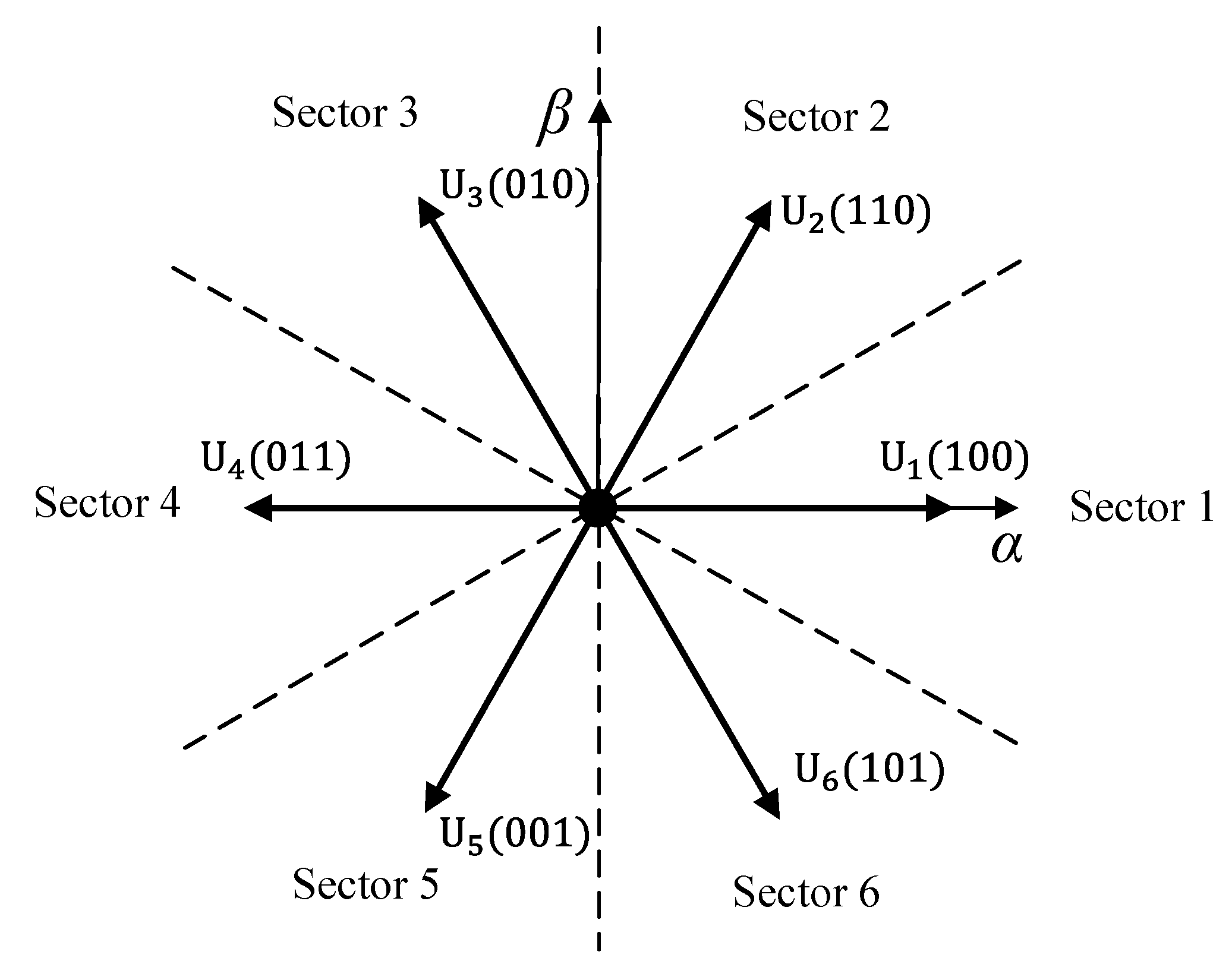
As shown in Figure 2, for the conventional DTC method, the plane is divided into six sectors. Taking sector 1 as an example, U₁, U₂ or U₃ can be selected to increase ${\mathsf{\psi }}_{\mathrm{s}}$. Conversely, a decrease can be obtained by selecting U₃, U₄ or U₅. To increase $\mathrm{T}$, voltage vectors U₂, U₃ or U₄ can be selected. A reduction in $\mathrm{T}$ can be obtained by selecting U₁, U₅ or U₆.

3. DTC–SVM Principles

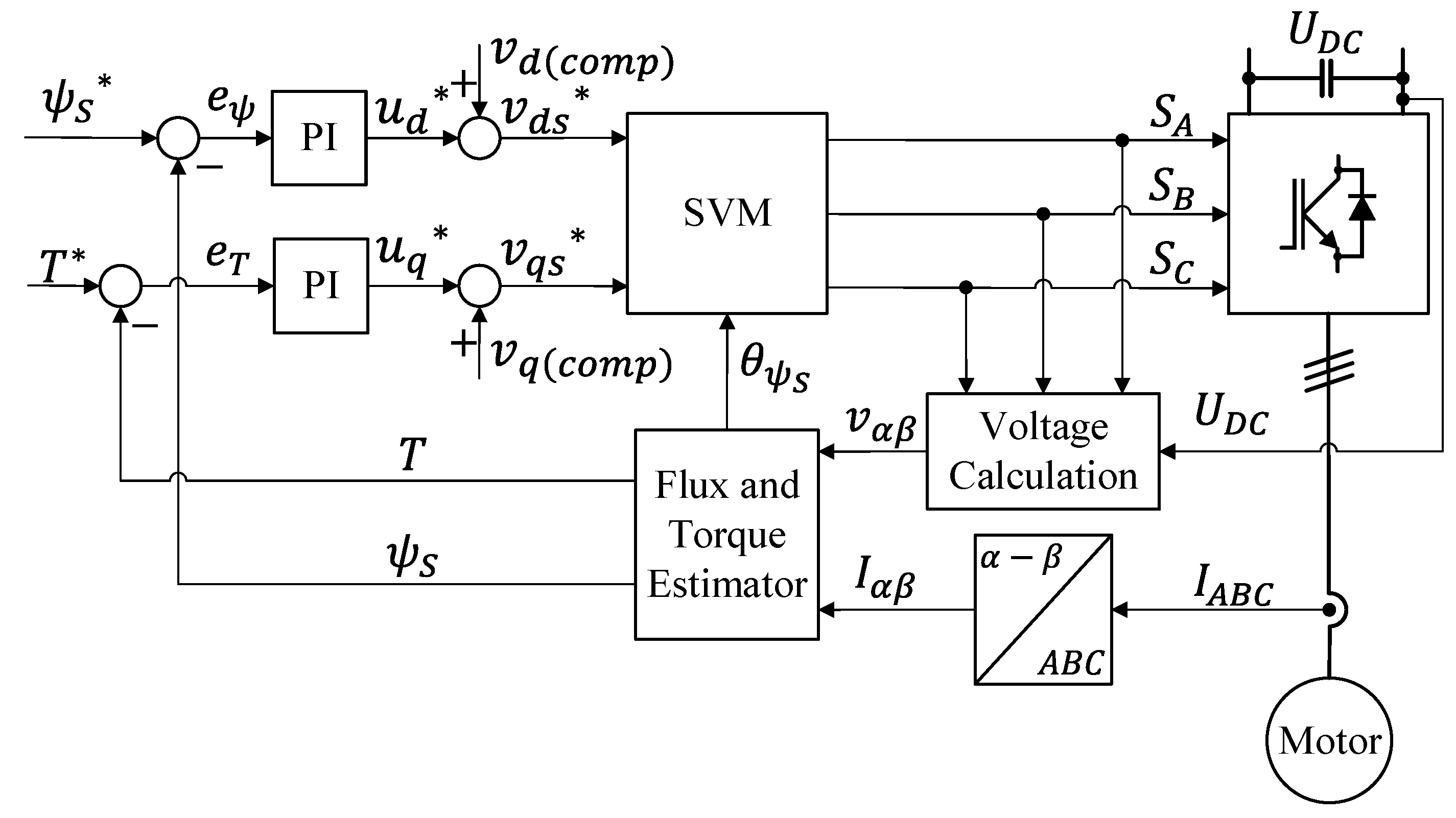
Among the different DTC–SVM methods that can be found in the literature, the scheme proposed in [37] is applied in this study. This scheme provides PI based close-loop torque and flux control in stator flux coordinate system. Its block diagram can be found in Figure 3. For this control method, the error between $\mathrm{T}$ and ${\mathrm{T}}^{*}$ is used as the input for torque PI controller. Similarly, the error between ${\mathsf{\psi }}_{\mathrm{s}}$ and ${\mathsf{\psi }}_{\mathrm{s}}{}^{*}$ is used as the input of the flux PI controller. After the decoupling terms compensation, the stator voltage reference components ${\mathrm{v}}_{\mathrm{ds}}{}^{*}$ and ${\mathrm{v}}_{\mathrm{qs}}{}^{*}$ in the stator flux-oriented coordinates $\left(\mathrm{d}-\mathrm{q}\right)$ can be obtained. The reference voltages ${\mathrm{v}}_{\mathrm{ds}}{}^{*}$ and ${\mathrm{v}}_{\mathrm{qs}}{}^{*}$ are then used as the input for the SVM to generate the inverter output pulses S_A, S_B and S_C.

With the stator flux-oriented scheme, $\overrightarrow{{\mathsf{\psi }}_{\mathrm{ds}}}=\overrightarrow{{\mathsf{\psi }}_{\mathrm{s}}}$ and $\overrightarrow{{\mathsf{\psi }}_{\mathrm{qs}}}=0$. The machine equations in the stator flux-oriented coordinates $\left(\mathrm{d}-\mathrm{q}\right)$ are:

$${\mathrm{v}}_{\mathrm{ds}}={\mathrm{R}}_{\mathrm{s}}{\mathrm{i}}_{\mathrm{ds}}+\frac{{\mathrm{d}\mathsf{\psi }}_{\mathrm{s}}}{\mathrm{dt}}$$

(1)

$${\mathrm{v}}_{\mathrm{qs}}={\mathrm{R}}_{\mathrm{s}}{\mathrm{i}}_{\mathrm{qs}}+{\mathsf{\omega }}_{\mathrm{s}}{\mathsf{\psi }}_{\mathrm{s}}$$

(2)

$$0={\mathrm{R}}_{\mathrm{r}}{\mathrm{i}}_{\mathrm{dr}}+\frac{{\mathrm{d}\mathsf{\psi }}_{\mathrm{dr}}}{\mathrm{dt}}-{\mathsf{\omega }}_{\mathrm{sl}}{\mathsf{\psi }}_{\mathrm{qr}}$$

(3)

$$0={\mathrm{R}}_{\mathrm{r}}{\mathrm{i}}_{\mathrm{qr}}+\frac{{\mathrm{d}\mathsf{\psi }}_{\mathrm{qr}}}{\mathrm{dt}}+{\mathsf{\omega }}_{\mathrm{sl}}{\mathsf{\psi }}_{\mathrm{dr}}$$

(4)

$${\mathsf{\psi }}_{\mathrm{s}}={\mathrm{L}}_{\mathrm{s}}{\mathrm{i}}_{\mathrm{ds}}+{\mathrm{L}}_{\mathrm{m}}{\mathrm{i}}_{\mathrm{dr}}$$

(5)

$$0={\mathrm{L}}_{\mathrm{s}}{\mathrm{i}}_{\mathrm{qs}}+{\mathrm{L}}_{\mathrm{m}}{\mathrm{i}}_{\mathrm{qr}}$$

(6)

$${\mathsf{\psi }}_{\mathrm{dr}}={\mathrm{L}}_{\mathrm{m}}{\mathrm{i}}_{\mathrm{ds}}+{\mathrm{L}}_{\mathrm{r}}{\mathrm{i}}_{\mathrm{dr}}$$

(7)

$${\mathsf{\psi }}_{\mathrm{qr}}={\mathrm{L}}_{\mathrm{m}}{\mathrm{i}}_{\mathrm{qs}}+{\mathrm{L}}_{\mathrm{r}}{\mathrm{i}}_{\mathrm{qr}}$$

(8)

$$\mathrm{T}=\frac{3}{2}{\mathrm{P}}_{\mathrm{P}}{\mathsf{\psi }}_{\mathrm{s}}{\mathrm{i}}_{\mathrm{qs}}$$

(9)

4. SVM-DTC Torque and Flux Transfer Functions

In this section, based on (1)–(9), the flux and torque transfer functions as well as the flux and torque decoupling terms are explained. Additionally, a simplified decoupling method is proposed.

4.1. Flux Transfer Function

Combining (1)–(9), the following equation is obtained:

$$\left({\mathrm{R}}_{\mathrm{r}}{\mathrm{L}}_{\mathrm{s}}+{\mathsf{\sigma }\mathrm{L}}_{\mathrm{s}}{\mathrm{L}}_{\mathrm{r}}\frac{\mathrm{d}}{\mathrm{dt}}\right){\mathrm{v}}_{\mathrm{ds}}=\left[{\mathrm{R}}_{\mathrm{s}}{\mathrm{R}}_{\mathrm{r}}+\frac{\mathrm{d}}{\mathrm{dt}}\left({\mathrm{R}}_{\mathrm{r}}{\mathrm{L}}_{\mathrm{s}}+{\mathrm{R}}_{\mathrm{s}}{\mathrm{L}}_{\mathrm{r}}\right)+{\mathsf{\sigma }\mathrm{L}}_{\mathrm{s}}{\mathrm{L}}_{\mathrm{r}}{\left(\frac{\mathrm{d}}{\mathrm{dt}}\right)}^2\right]{\mathsf{\psi }}_{\mathrm{s}}+{\mathrm{R}}_{\mathrm{s}}{\mathrm{i}}_{\mathrm{qs}}{\mathsf{\sigma }\mathrm{L}}_{\mathrm{s}}{\mathrm{L}}_{\mathrm{r}}{\mathsf{\omega }}_{\mathrm{sl}}$$

(10)

where, $\mathsf{\sigma }=1-\frac{{\mathrm{L}}_{\mathrm{m}}{}^2}{{\mathrm{L}}_{\mathrm{s}}{\mathrm{L}}_{\mathrm{r}}}$.

Isolating ${\mathrm{v}}_{\mathrm{ds}}$ in (10) and applying the Laplace transformation, ${\mathrm{v}}_{\mathrm{ds}}$ can be expressed as:

$${\mathrm{v}}_{\mathrm{ds}}=\frac{{\mathrm{R}}_{\mathrm{s}}{\mathrm{R}}_{\mathrm{r}}+\left({\mathrm{R}}_{\mathrm{r}}{\mathrm{L}}_{\mathrm{s}}+{\mathrm{R}}_{\mathrm{s}}{\mathrm{L}}_{\mathrm{r}}\right)\mathrm{S}+{\mathsf{\sigma }\mathrm{L}}_{\mathrm{s}}{\mathrm{L}}_{\mathrm{r}}{\mathrm{S}}^2}{{\mathrm{R}}_{\mathrm{r}}{\mathrm{L}}_{\mathrm{s}}+{\mathsf{\sigma }\mathrm{L}}_{\mathrm{s}}{\mathrm{L}}_{\mathrm{r}}\mathrm{S}}{\mathsf{\psi }}_{\mathrm{s}}+\frac{{\mathrm{R}}_{\mathrm{s}}\frac{{\mathsf{\sigma }\mathrm{L}}_{\mathrm{r}}}{{\mathrm{R}}_{\mathrm{r}}}}{\frac{{\mathsf{\sigma }\mathrm{L}}_{\mathrm{r}}}{{\mathrm{R}}_{\mathrm{r}}}\mathrm{S}+1}{\mathrm{i}}_{\mathrm{qs}}{\mathsf{\omega }}_{\mathrm{sl}}={\mathrm{u}}_{\mathrm{ds}}+{\mathrm{v}}_{\mathrm{ds}\left(\mathrm{comp}\right)}$$

(11)

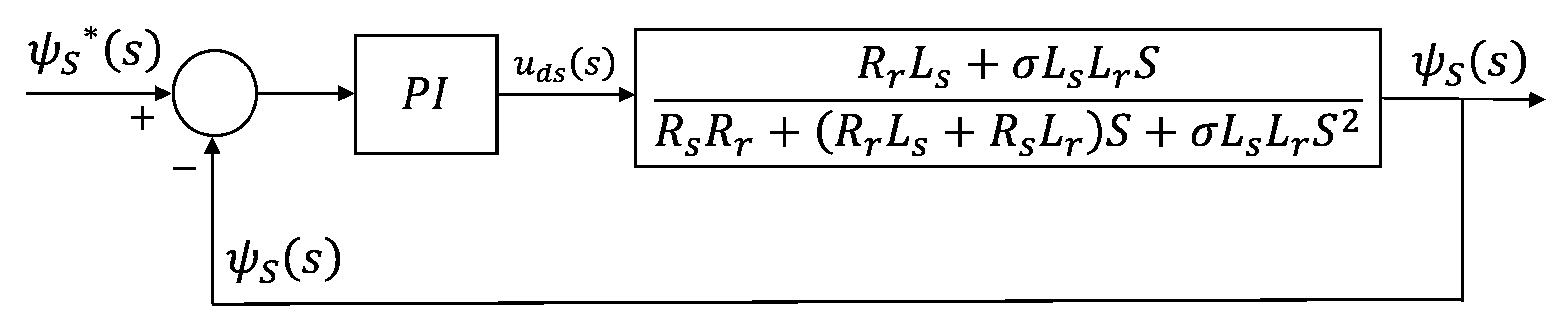
which can be rewritten as:

$$\frac{{\mathsf{\psi }}_{\mathrm{s}}}{{\mathrm{v}}_{\mathrm{ds}}-{\mathrm{v}}_{\mathrm{ds}\left(\mathrm{comp}\right)}}=\frac{{\mathsf{\psi }}_{\mathrm{s}}}{{\mathrm{u}}_{\mathrm{ds}}}=\frac{{\mathrm{R}}_{\mathrm{r}}{\mathrm{L}}_{\mathrm{s}}+{\mathsf{\sigma }\mathrm{L}}_{\mathrm{s}}{\mathrm{L}}_{\mathrm{r}}\mathrm{S}}{{\mathrm{R}}_{\mathrm{s}}{\mathrm{R}}_{\mathrm{r}}+\left({\mathrm{R}}_{\mathrm{r}}{\mathrm{L}}_{\mathrm{s}}+{\mathrm{R}}_{\mathrm{s}}{\mathrm{L}}_{\mathrm{r}}\right)\mathrm{S}+{\mathsf{\sigma }\mathrm{L}}_{\mathrm{s}}{\mathrm{L}}_{\mathrm{r}}{\mathrm{S}}^2}$$

(12)

where ${\mathrm{v}}_{\mathrm{ds}\left(\mathrm{comp}\right)}$ is the flux decoupling compensation and ${\mathrm{u}}_{\mathrm{ds}}$ is the flux PI controller output.

Hence, the block diagram shown in Figure 4 is obtained:

4.2. Flux Decoupling Compensation

Equation (11) shows ${\mathrm{v}}_{\mathrm{ds}\left(\mathrm{comp}\right)}$ is dependent on the slip speed $\left({\mathsf{\omega }}_{\mathrm{sl}}\right)$. Rearranging (1)–(9) and applying a Laplace transformation, the following expression can be obtained for ${\mathsf{\omega }}_{\mathrm{sl}}$:

$${\mathsf{\omega }}_{\mathrm{sl}}=\frac{\left(\mathrm{S}+\frac{1}{{\mathsf{\sigma }\mathsf{\tau }}_{\mathrm{r}}}\right){\mathrm{i}}_{\mathrm{qs}}}{\frac{{\mathsf{\psi }}_{\mathrm{S}}}{{\mathsf{\sigma }\mathrm{L}}_{\mathrm{s}}}-{\mathrm{i}}_{\mathrm{ds}}}$$

(13)

where ${\mathsf{\tau }}_{\mathrm{r}}=\frac{{\mathrm{L}}_{\mathrm{r}}}{{\mathrm{R}}_{\mathrm{r}}}$.

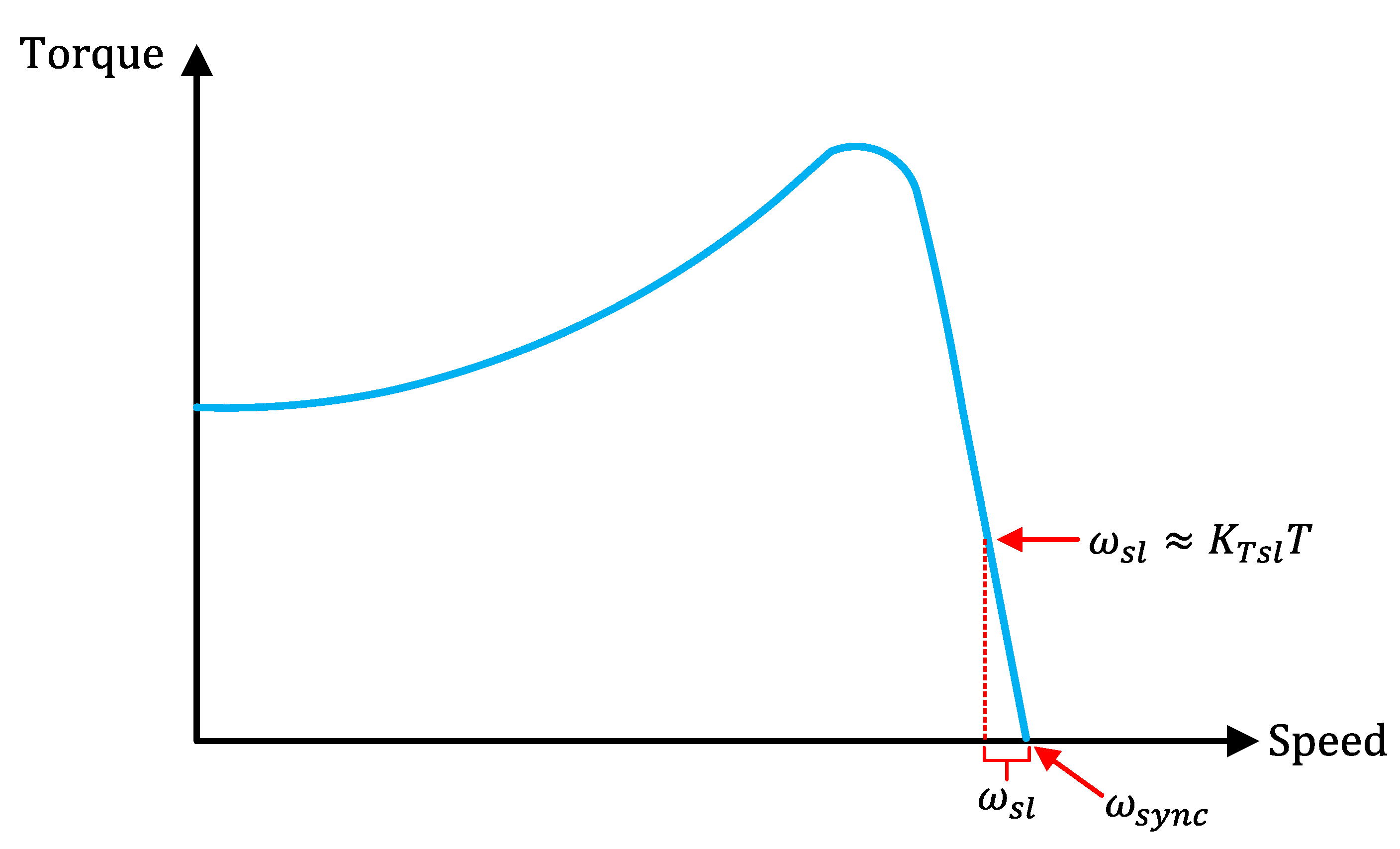
Based on (13), the calculation of ${\mathsf{\omega }}_{\mathrm{sl}}$ requires the differentiation of ${\mathrm{i}}_{\mathrm{qs}}$, where it is disadvantageous compared to the rotor flux-oriented scheme due to the increased sensitivity to the noise. However, the calculation of ${\mathrm{v}}_{\mathrm{ds}\left(\mathrm{comp}\right)}$ can be simplified using the following assumptions:

• Under steady-state conditions, ${\mathsf{\psi }}_{\mathrm{s}}$ is constant and equal to its reference $\left({\mathsf{\psi }}_{\mathrm{s}}={ \mathsf{\psi }}_{\mathrm{s}}{}^{*}\right).$
• Under steady-state conditions, $\mathrm{T}$ is constant and equal to its reference $\left(\mathrm{T}={ \mathrm{T}}^{*}\right).$
• According to Figure 5, if it is considered that within the IM working region, the slope for $\mathrm{T}$ is constant $\left({\mathrm{K}}_{\mathrm{Tsl}}\right)$, the slip speed can be approximated by ${\mathsf{\omega }}_{\mathrm{sl}}\approx {\mathrm{K}}_{\mathrm{Tsl}}{\mathrm{T}}^{*}$, avoiding the differentiation of ${\mathrm{i}}_{\mathrm{qs}}$.

In (11), ${\mathrm{v}}_{\mathrm{ds}\left(\mathrm{comp}\right)}$ has the characteristic of a low-pass filter. Hence, assuming the frequency response of this filter is considerably faster than the dynamic of ${\mathrm{T}}^{*}$, the following approximation can be used:

$$\frac{{\mathrm{R}}_{\mathrm{s}}\frac{{\mathsf{\sigma }\mathrm{L}}_{\mathrm{r}}}{{\mathrm{R}}_{\mathrm{r}}}}{\frac{{\mathsf{\sigma }\mathrm{L}}_{\mathrm{r}}}{{\mathrm{R}}_{\mathrm{r}}}\mathrm{S}+1}\approx {\mathrm{R}}_{\mathrm{s}}\frac{{\mathsf{\sigma }\mathrm{L}}_{\mathrm{r}}}{{\mathrm{R}}_{\mathrm{r}}}$$

(14)

Taking (9) and considering the assumptions above, the following simplified expression can be obtained for ${\mathrm{v}}_{\mathrm{ds}\left(\mathrm{comp}\right)}$:

$${\mathrm{v}}_{\mathrm{ds}\left(\mathrm{comp}\right)}\approx \frac{2{\mathrm{R}}_{\mathrm{s}}{\mathsf{\sigma }\mathrm{L}}_{\mathrm{r}}{\mathrm{K}}_{\mathrm{Tsl}}{\mathrm{T}}^{*}{}^2}{3{\mathrm{R}}_{\mathrm{r}}{\mathrm{P}}_{\mathrm{P}}{\mathsf{\psi }}_{\mathrm{s}}{}^{*}}$$

(15)

As can be seen in (15), since ${\mathsf{\psi }}_{\mathrm{s}}{}^{*}$ is assumed to be constant, the only variable is ${\mathrm{T}}^{*}$.

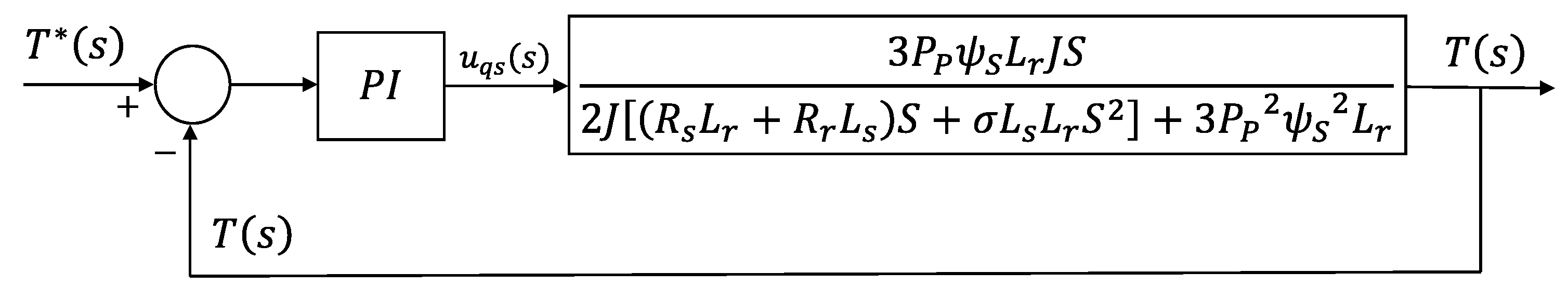
4.3. Torque Transfer Function

Based on motor model Equations (1)–(9), the following equation can be obtained:

$$\left[\left({\mathrm{R}}_{\mathrm{s}}{\mathrm{L}}_{\mathrm{r}}+{\mathrm{R}}_{\mathrm{r}}{\mathrm{L}}_{\mathrm{s}}\right)+{\mathsf{\sigma }\mathrm{L}}_{\mathrm{s}}{\mathrm{L}}_{\mathrm{r}}\frac{\mathrm{d}}{\mathrm{dt}}\right]{\mathrm{i}}_{\mathrm{qs}}={\mathrm{L}}_{\mathrm{r}}{\mathrm{v}}_{\mathrm{qs}}-{\mathrm{L}}_{\mathrm{r}}{\mathsf{\psi }}_{\mathrm{s}}{\mathrm{P}}_{\mathrm{P}}{\mathsf{\omega }}_{\mathrm{mech}}+{ \mathrm{i}}_{\mathrm{ds}}{\mathsf{\sigma }\mathrm{L}}_{\mathrm{s}}{\mathrm{L}}_{\mathrm{r}}{\mathsf{\omega }}_{\mathrm{sl}}$$

(16)

Assuming the dynamic of the mechanical load is significantly slower than the torque controller response, the mechanical rotor speed can be expressed as:

$$\frac{{\mathrm{d}\mathsf{\omega }}_{\mathrm{mech}}}{\mathrm{dt}}=\frac{1}{\mathrm{J}}\mathrm{T}$$

(17)

Combining (9), (16) and (17), isolating ${\mathrm{v}}_{\mathrm{qs}}$ and applying the Laplace transformation, the following equation is obtained:

$${\mathrm{v}}_{\mathrm{qs}}=\left\{\frac{2\mathrm{J}\left[\left({\mathrm{R}}_{\mathrm{s}}{\mathrm{L}}_{\mathrm{r}}+{\mathrm{R}}_{\mathrm{r}}{\mathrm{L}}_{\mathrm{s}}\right)\mathrm{S}+{\mathsf{\sigma }\mathrm{L}}_{\mathrm{s}}{\mathrm{L}}_{\mathrm{r}}{\mathrm{S}}^2\right]+3{\mathrm{P}}_{\mathrm{P}}{}^2{\mathsf{\psi }}_{\mathrm{s}}{}^2{\mathrm{L}}_{\mathrm{r}}}{3{\mathrm{P}}_{\mathrm{P}}{\mathsf{\psi }}_{\mathrm{s}}{\mathrm{L}}_{\mathrm{r}}\mathrm{JS}}\right\}\mathrm{T}-{\mathsf{\sigma }\mathrm{L}}_{\mathrm{s}}{\mathrm{i}}_{\mathrm{ds}}{\mathsf{\omega }}_{\mathrm{sl}}={\mathrm{u}}_{\mathrm{qs}}+{\mathrm{v}}_{\mathrm{qs}\left(\mathrm{comp}\right)}$$

(18)

where, ${\mathrm{v}}_{\mathrm{qs}\left(\mathrm{comp}\right)}$ is the torque decoupling compensation and ${\mathrm{u}}_{\mathrm{qs}}$ is the torque PI controller output.

This can be rewritten as:

$$\frac{\mathrm{T}}{{\mathrm{v}}_{\mathrm{qs}}-{\mathrm{v}}_{\mathrm{qs}\left(\mathrm{comp}\right)}}=\frac{\mathrm{T}}{{\mathrm{u}}_{\mathrm{qs}}}=\frac{3{\mathrm{P}}_{\mathrm{P}}{\mathsf{\psi }}_{\mathrm{s}}{\mathrm{L}}_{\mathrm{r}}\mathrm{JS}}{2\mathrm{J}\left[\left({\mathrm{R}}_{\mathrm{s}}{\mathrm{L}}_{\mathrm{r}}+{\mathrm{R}}_{\mathrm{r}}{\mathrm{L}}_{\mathrm{s}}\right)\mathrm{S}+{\mathsf{\sigma }\mathrm{L}}_{\mathrm{s}}{\mathrm{L}}_{\mathrm{r}}{\mathrm{S}}^2\right]+3{\mathrm{P}}_{\mathrm{P}}{}^2{\mathsf{\psi }}_{\mathrm{s}}{}^2{\mathrm{L}}_{\mathrm{r}}}$$

(19)

Hence, the block diagram shown in Figure 6 is obtained:

4.4. Torque Decoupling Compensation

As shown in (18), ${\mathrm{v}}_{\mathrm{qs}\left(\mathrm{comp}\right)}=-{\mathsf{\sigma }\mathrm{L}}_{\mathrm{s}}{\mathrm{i}}_{\mathrm{ds}}{\mathsf{\omega }}_{\mathrm{sl}}$. However, as experimental results demonstrate in Figure 19, the contribution of this term is negligible (typically less than 1% of ${\mathrm{v}}_{\mathrm{qs}}$). Hence, ${\mathrm{v}}_{\mathrm{qs}\left(\mathrm{comp}\right)}$ is neglected and it is considered that ${\mathrm{u}}_{\mathrm{qs}}={\mathrm{v}}_{\mathrm{qs}}$.

5. Stator Flux Estimation

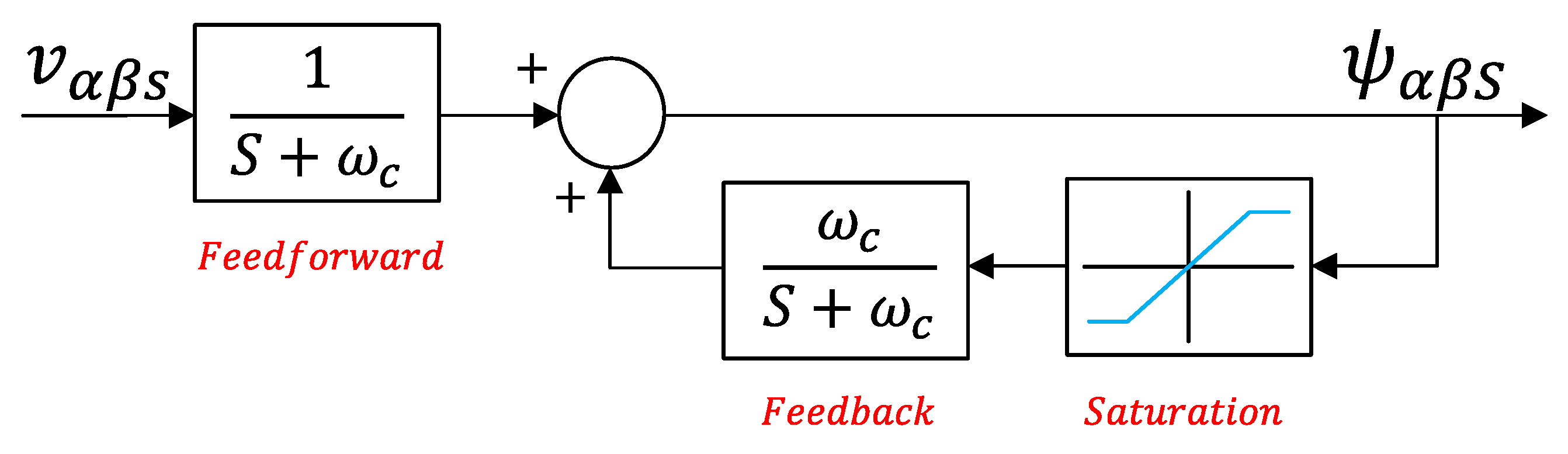
Theoretically, the stator flux could be determined by integrating the electromagnetic force of the motor by ${\mathsf{\psi }}_{\mathrm{s}}={\int }^{}\left({\mathrm{v}}_{\mathsf{\alpha }\mathsf{\beta }}-{\mathrm{R}}_{\mathrm{s}}{\mathrm{i}}_{\mathsf{\alpha }\mathsf{\beta }}\right)\mathrm{dt}$. However, the implementation of an integrator for motor flux estimation has dc drift and initial value problems. Even a small portion of this dc offset can drive a pure integrator into saturation [38]. In the literature, different methods based on the “voltage model” are used to modify the integrators and remove the dc drift problem. The method “Algorithm 1” proposed in [38] is implemented in this study. This method offers good results, easy implementation, and complete independence from motor parameters. The block diagram of this stator flux estimator is shown in Figure 7.

Based on this algorithm, ${\mathsf{\psi }}_{\mathrm{s}}$ can be obtained by ${\mathsf{\psi }}_{\mathrm{s}}=\sqrt{\left({\mathsf{\psi }}_{\mathsf{\alpha }\mathrm{s}}{}^2+{\mathsf{\psi }}_{\mathsf{\beta }\mathrm{s}}{}^2\right)}$, and the estimated stator flux angle $\left({\mathsf{\theta }}_{{\mathsf{\psi }}_{\mathrm{s}}}\right)$ by ${\mathsf{\theta }}_{{\mathsf{\psi }}_{\mathrm{s}}}={\tan }^{-1}\left({\mathsf{\psi }}_{\mathsf{\beta }\mathrm{s}}/{\mathsf{\psi }}_{\mathsf{\alpha }\mathrm{s}}\right)$. However, due to the nonlinearities such as switch voltage drops, PWM dead-time and digital-control delays, the estimation accuracy of the stator flux angle is degraded, causing $\overrightarrow{{\mathsf{\psi }}_{\mathrm{s}}}$ to not be perfectly aligned with the d-axis. This misalignment results in the imperfect decoupling between torque and flux.

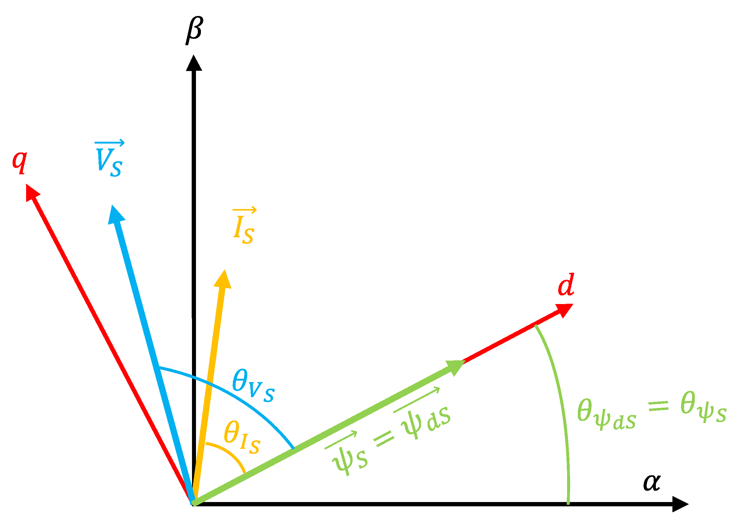
Compensation of the Nonlinearities Affecting the Stator Flux Angle Estimation

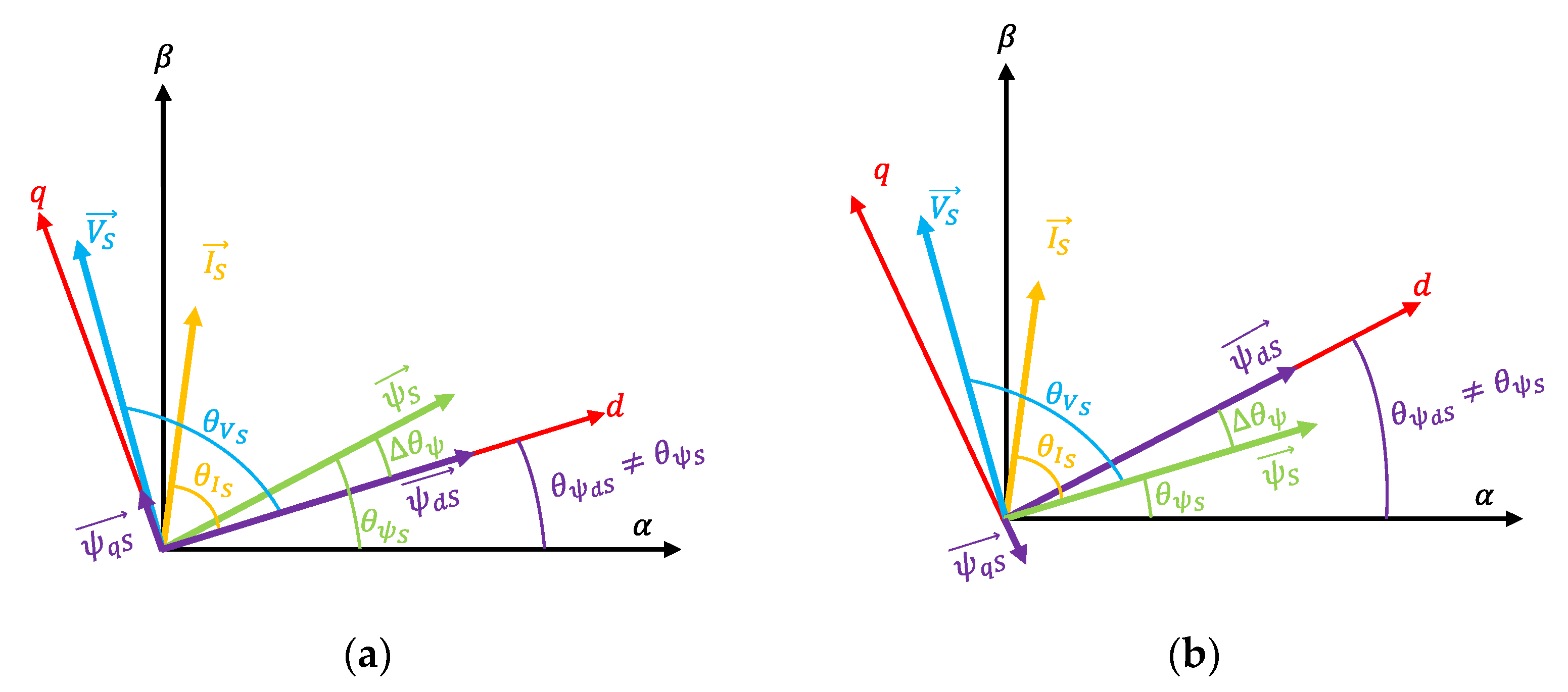
Assuming a perfect stator flux angle estimation $\left({\mathsf{\theta }}_{{\mathsf{\psi }}_{\mathrm{ds}}}={\mathsf{\theta }}_{{\mathsf{\psi }}_{\mathrm{s}}}\right)$, as shown in Figure 8.

However, due to the nonlinearities mentioned above, $\overrightarrow{{\mathsf{\psi }}_{\mathrm{s}}}$ is not perfectly aligned with the d-axis. Figure 9a,b shows the situation where the d-axis is lagging behind and ahead of the stator flux vector, respectively.

Under non-ideal conditions, ${\mathsf{\psi }}_{\mathrm{qs}}$ is not zero, as can be seen in Figure 9a,b. Hence, instead of having (1), for this non-ideal situation, the following equation is obtained:

$${\mathrm{v}}_{\mathrm{ds}}={\mathrm{R}}_{\mathrm{s}}{\mathrm{i}}_{\mathrm{ds}}+\frac{{\mathrm{d}\mathsf{\psi }}_{\mathrm{ds}}}{\mathrm{dt}}-{\mathsf{\omega }}_{\mathrm{sync}}{\mathsf{\psi }}_{\mathrm{qs}}$$

(20)

The principle of this misalignment correction method is to make sure that ${\mathsf{\psi }}_{\mathrm{qs}}$ is zero. Considering the steady-state condition $\left({\mathrm{d}\mathsf{\psi }}_{\mathrm{ds}}/\mathrm{dt}=0\right)$, to achieve perfect alignment of the d-axis, the following condition must be obtained:

$${\mathrm{v}}_{\mathrm{ds}}={\mathrm{R}}_{\mathrm{s}}{\mathrm{i}}_{\mathrm{ds}}$$

(21)

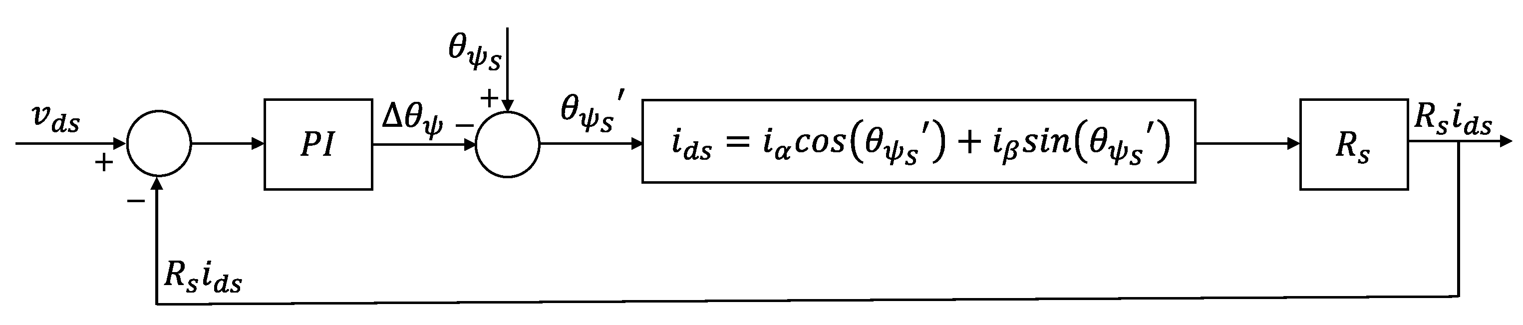
Hence, we propose an additional control loop that generates the required angle to correct the misalignment $\left(\Delta {\mathsf{\theta }}_{\mathsf{\psi }}\right)$. $\Delta {\mathsf{\theta }}_{\mathsf{\psi }}$ is subtracted from ${\mathsf{\theta }}_{{\mathsf{\psi }}_{\mathrm{s}}}$, resulting in a corrected value of the estimated stator flux angle $\left({\mathsf{\theta }}_{{\mathsf{\psi }}_{\mathrm{s}}}{}^{\prime }\right)$:

$${\mathsf{\theta }}_{{\mathsf{\psi }}_{\mathrm{s}}}{}^{\prime }={\mathsf{\theta }}_{{\mathsf{\psi }}_{\mathrm{s}}}-\Delta {\mathsf{\theta }}_{\mathsf{\psi }}$$

(22)

The block diagram of this extra loop can be found in Figure 10:

Note that for this control method, a change in $\Delta {\mathsf{\theta }}_{\mathsf{\psi }}$ has the same effect for ${\mathrm{v}}_{\mathrm{ds}}$ and ${\mathrm{i}}_{\mathrm{ds}}$. It means that both ${\mathrm{v}}_{\mathrm{ds}}$ and ${\mathrm{i}}_{\mathrm{ds}}$ increase by increasing $\Delta {\mathsf{\theta }}_{\mathsf{\psi }}$. However, not in the same proportion. As can be seen in the experimental results (Figures 16–19), for stator flux-orientation, the ratio of stator voltage corresponding to the d-axis $\left({\mathrm{v}}_{\mathrm{ds}}\right)$ is larger than the ratio of stator current that corresponds to the d-axis $\left({\mathrm{i}}_{\mathrm{ds}}\right)$. In other words:

$$\frac{\left|{\mathrm{i}}_{\mathrm{qs}}\right|}{\left|{\mathrm{i}}_{\mathrm{ds}}\right|}<\frac{\left|{\mathrm{v}}_{\mathrm{qs}}\right|}{\left|{\mathrm{v}}_{\mathrm{ds}}\right|}$$

(23)

If, then, an increase in $\Delta {\mathsf{\theta }}_{\mathsf{\psi }}$ takes place, it will result in the increase of both ${\mathrm{v}}_{\mathrm{ds}}$ and ${\mathrm{i}}_{\mathrm{ds}}$. However, the proportion of the ${\mathrm{i}}_{\mathrm{ds}}$ increment is smaller than the ${\mathrm{v}}_{\mathrm{ds}}$ increment.

To guarantee the stability of the system, if the inequality in (23) is not fulfilled, $\Delta {\mathsf{\theta }}_{\mathsf{\psi }}$ is then set to zero.

Ensuring the stability of the flux loop, the PI of the proposed control loop must be designed to have a slower transient response than the flux loop. Yet, to ensure fast torque response, it must be faster than the change ratio of the torque command.

6. DC Bus Utilization Limits

In square-wave or six-step operation mode, the phase voltage $\left({\mathrm{U}}_{\mathrm{A}}\right)$ of an inverter fed motor can be expressed by a Fourier series as in [32]:

$${\mathrm{U}}_{\mathrm{A}}=\frac{2}{\mathsf{\pi }}{\mathrm{U}}_{\mathrm{DC}}{\displaystyle \sum }_{\mathrm{n}=1}^{\infty }\frac{1}{\mathrm{n}}\sin \left(\mathrm{n}\mathsf{\omega }\mathrm{t}\right)$$

(24)

From (24), the fundamental peak value of the phase voltage $\left({\mathrm{U}}_{\mathrm{pk}}\right)$ is given as:

$${\mathrm{U}}_{\mathrm{pk}}=\frac{2}{\mathsf{\pi }}{\mathrm{U}}_{\mathrm{DC}}$$

(25)

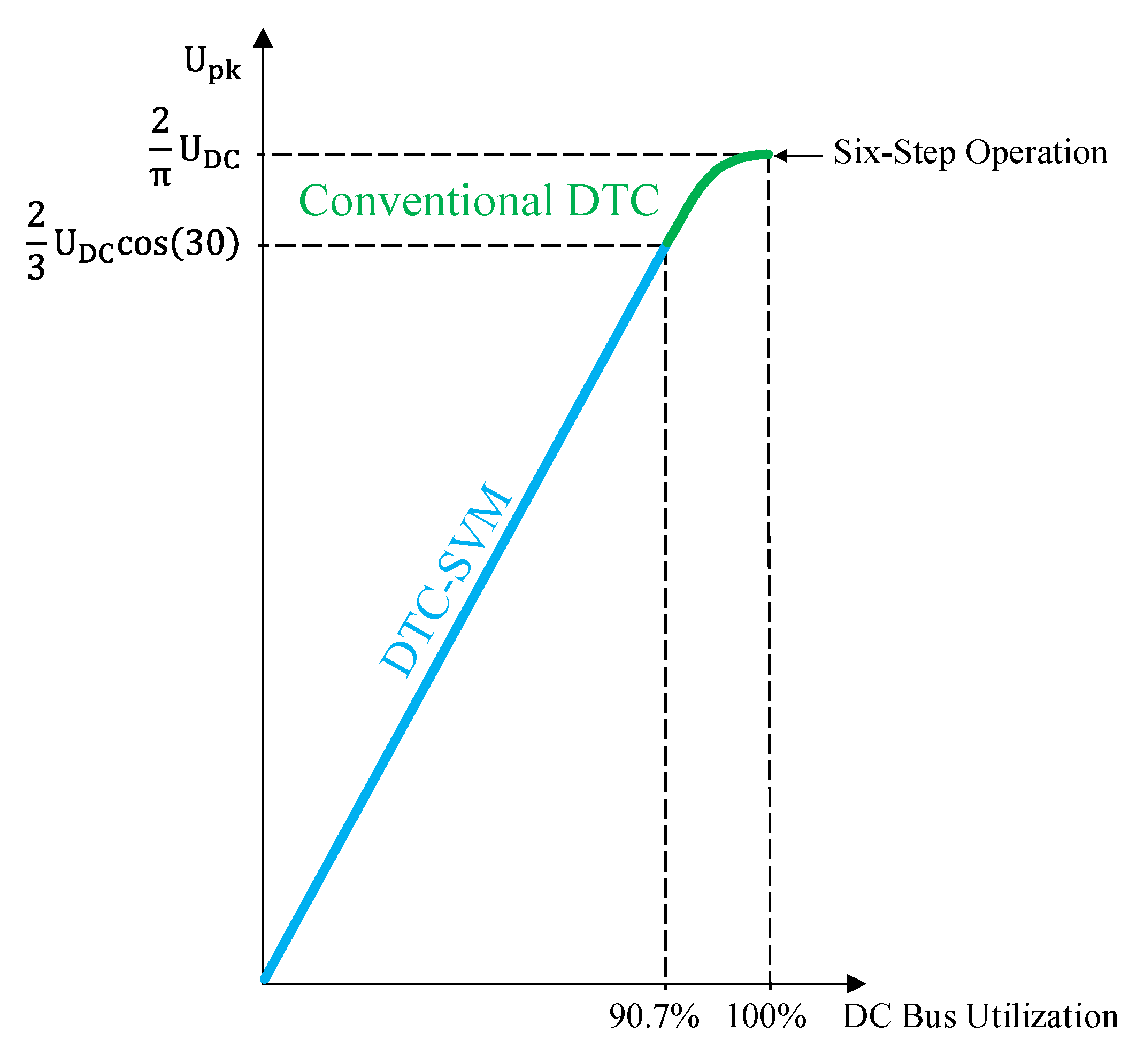
However, when linear modulation mode is applied, (25) cannot be attained. Linear modulation strategies, such as SVPWM, can provide a maximum ${\mathrm{U}}_{\mathrm{pk}}$ in the linear region equal to $\left(2/3\right){\mathrm{U}}_{\mathrm{DC}}\cos \left(30\right)\approx 0.577{\mathrm{U}}_{\mathrm{DC}}.$ It corresponds to the 90.7% of the value given by (25). Controller saturation occurs when phase voltage beyond the limit is required. To extend the voltage capability, overmodulation algorithms are required. Nevertheless, such approaches have several disadvantages: complex computational effort, increased current harmonics, and degraded controllability that results in poor transient behavior [32,33,34].

7. Combination of DTC–SVM and Conventional DTC

SVPWM has the advantages of constant switching frequency, low THD, low switching losses and low torque ripple. However, the maximum ${\mathrm{U}}_{\mathrm{pk}}$ is limited to 90.7% of the value given by (25), leaving some of the DC bus voltage as unusable. On the other hand, conventional DTC can exploit 100% of the DC bus capability, with the drawbacks, however, of higher THD and torque ripple than DTC–SVM.

The control algorithm proposed in this paper aims to exploit the advantages of both DTC–SVM and conventional DTC. In order to do that, DTC–SVM is applied during the linear region, until ${\mathrm{U}}_{\mathrm{pk}}=\left(2/3\right){\mathrm{U}}_{\mathrm{DC}}\cos \left(30\right).$ Controller saturation occurs when operation beyond this limit is required. To ensure continuous controllability, the control scheme is then switched to conventional DTC, allowing it to exploit 100% of the DC bus capability. The selection of which control method should be implemented is carried out from the value of ${\mathrm{U}}_{\mathrm{pk}}$ necessary to guarantee the controllability of ${\mathsf{\psi }}_{\mathrm{s}}$ and $\mathrm{T}$. If the required value of ${\mathrm{U}}_{\mathrm{pk}}$ can be obtained within the linear region, DTC–SVM will be implemented due to its better performance in the linear region. On the contrary, if said ${\mathrm{U}}_{\mathrm{pk}}$ value cannot be obtained within the linear region, conventional DTC will be implemented due to its better performance outside the linear region. In other words, while ${\mathrm{U}}_{\mathrm{pk}}$ is within the linear region limit, the control algorithm will select DTC–SVM to control ${\mathsf{\psi }}_{\mathrm{s}}$ and $\mathrm{T}$. However, when the operating conditions require a higher value of ${\mathrm{U}}_{\mathrm{pk}}$, which cannot be attained by DTC–SVM within the linear region, the control algorithm will select the conventional DTC to control ${\mathsf{\psi }}_{\mathrm{s}}$ and $\mathrm{T}$.

Figure 11 shows the operating regions of each control method, as well as the DC bus utilization and the value of ${\mathrm{U}}_{\mathrm{pk}}$ that can be obtained by each control method.

The scheme proposed in this paper allows for an instantaneous torque response up to 100% DC bus utilization without the drawbacks of complex computational effort, offline data computing, degraded controllability and poor transient behavior. The higher current distortion, characteristic of the conventional DTC, is justified at the overmodulation region, since the current distortion and torque ripple will increase regardless of which control method is used.

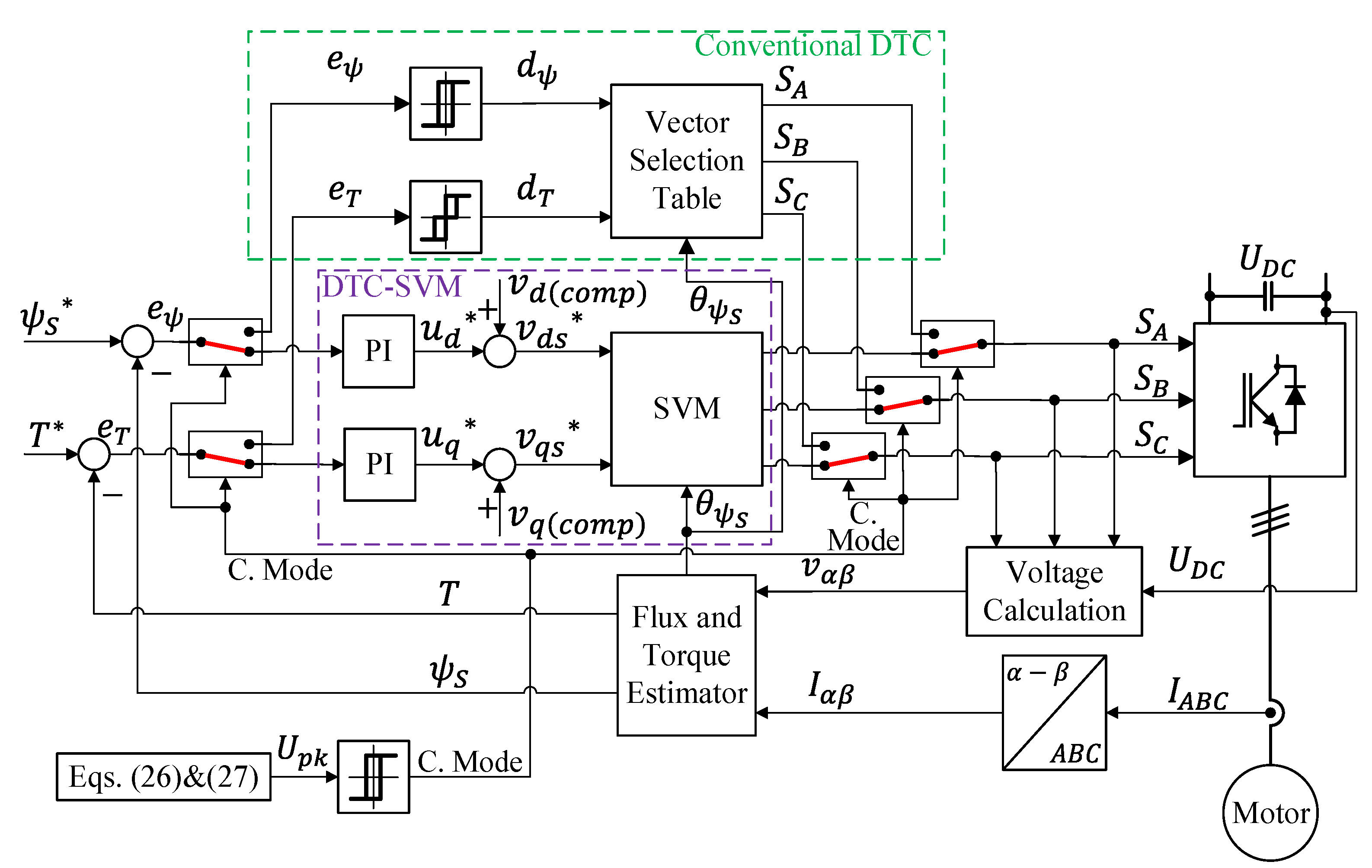
Figure 12 shows the complete control structure proposed in this paper. It consists of two selectable control methods. Both control methods share the same torque and flux estimators, as well as the same ${\mathrm{T}}^{*}$ and ${\mathsf{\psi }}_{\mathrm{s}}{}^{*}$.

As can be seen in Figure 12, DTC–SVM controls ${\mathsf{\psi }}_{\mathrm{s}}$ and $\mathrm{T}$ by means of two PI controllers. At the output of the PI controllers, ${\mathrm{v}}_{\mathrm{ds}\left(\mathrm{comp}\right)}$ and ${\mathrm{v}}_{\mathrm{qs}\left(\mathrm{comp}\right)}$ are added to decouple ${\mathsf{\psi }}_{\mathrm{S}}$ and $\mathrm{T}$. As a result, reference voltages ${\mathrm{v}}_{\mathrm{ds}}{}^{*}$ and ${\mathrm{v}}_{\mathrm{qs}}{}^{*}$ are then used as inputs for the SVM block to generate S_A, S_B, and S_C. Hence, when DTC–SVM is applied, the value of ${\mathrm{U}}_{\mathrm{pk}}$ necessary to guarantee the controllability of ${\mathsf{\psi }}_{\mathrm{s}}$ and $\mathrm{T}$ is obtained by (26). When the control algorithm implements conventional DTC, ${\mathsf{\psi }}_{\mathrm{s}}$ and $\mathrm{T}$ are controlled by means of two hysteretic controllers. In this situation, ${\mathrm{U}}_{\mathrm{pk}}$ is obtained from ${\mathrm{v}}_{\mathsf{\alpha }}$ and ${\mathrm{v}}_{\mathsf{\beta }}$ (27), which are reconstructed from S_A, S_B, S_C and ${\mathrm{U}}_{\mathrm{DC}}$ [38].

$${\mathrm{U}}_{\mathrm{pk}}=\sqrt{{\mathrm{v}}_{\mathrm{ds}}^{*}{}^2+{\mathrm{v}}_{\mathrm{qs}}^{*}{}^2}$$

(26)

$${\mathrm{U}}_{\mathrm{pk}}=\sqrt{{\mathrm{v}}_{\mathsf{\alpha }}{}^2+{\mathrm{v}}_{\mathsf{\beta }}{}^2}$$

(27)

8. Transition between Control Modes

To avoid oscillations between the two control methods, the selection of the control mode is done in a hysteretic fashion. The controller is switched from DTC–SVM to conventional DTC when ${\mathrm{U}}_{\mathrm{pk}}$ reaches the limit of the linear region $\left({\mathrm{U}}_{\mathrm{pk}}\ge 0.577{\mathrm{U}}_{\mathrm{DC}}\right)$. Conversely, the controller is switched from conventional DTC to DTC–SVM when ${\mathrm{U}}_{\mathrm{pk}}$ is below the 90% of the linear region limit $\left({\mathrm{U}}_{\mathrm{pk}}\le 0.52{\mathrm{U}}_{\mathrm{DC}}\right)$.

Due to the instantaneous response of the hysteretic controller used by the conventional DTC, the transition from DTC–SVM to conventional DTC is straightforward. However, when DTC–SVM is not selected, the torque and flux PI controllers must be prevented from accumulating error. To do that, during the transition and while conventional DTC is implemented, the integral term of the flux and torque PI controllers $\left({\mathrm{u}}_{{\mathrm{i}}_{{\mathsf{\psi }}_{\mathrm{s}}}} \mathrm{and} {\mathrm{u}}_{{\mathrm{i}}_{\mathrm{T}}}\right)$ are set to zero.

On the other hand, the transition from conventional DTC to DTC–SVM needs more consideration. In order to have a smooth transition, ${\mathrm{u}}_{{\mathrm{i}}_{{\mathsf{\psi }}_{\mathrm{s}}}}$ and ${\mathrm{u}}_{{\mathrm{i}}_{\mathrm{T}}}$ must be properly initialized at the time of the transition. The principle is that torque and flux controllers need to generate an output that will be translated into the same $\mathrm{T}$ and ${\mathsf{\psi }}_{\mathrm{s}}$ that was obtained for the last cycle of conventional DTC.

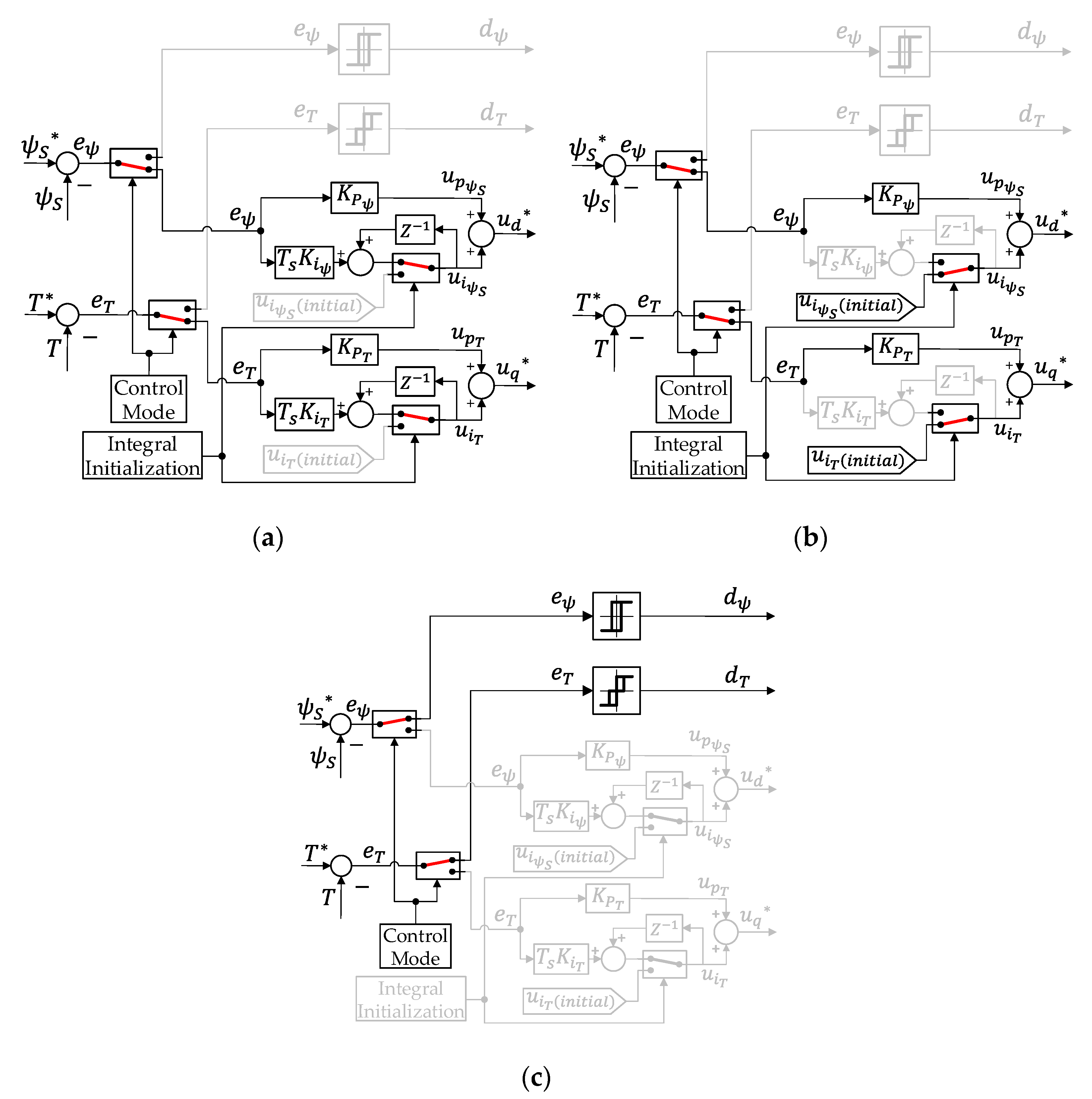
Figure 13a–c show in detail the controller architecture that is implemented in each region. Torque and flux PI controllers from Figure 12 have been discretized using the backward Euler rule [39]. Furthermore, the integral terms initialization during the transition from conventional DTC to DTC–SVM $\left({\mathrm{u}}_{{\mathrm{i}}_{{\mathsf{\psi }}_{\mathrm{s}}}\left(\mathrm{initial}\right)} \mathrm{and} {\mathrm{u}}_{{\mathrm{i}}_{\mathrm{T}}\left(\mathrm{initial}\right)}\right)$ has also been included. Figure 13a shows the normal operation for DTC–SVM. In this situation, PI controllers don’t have any modifications. From the whole control structure, conventional DTC and integral initialization signals are deactivated. Figure 13b shows the control structure at the transition from conventional DTC to DTC–SVM. In this situation, conventional DTC is deactivated, whereas the integral initialization signal is activated. Regarding the flux and torque PI controllers, ${\mathrm{u}}_{{\mathrm{i}}_{{\mathsf{\psi }}_{\mathrm{s}}}}$ and ${\mathrm{u}}_{{\mathrm{i}}_{\mathrm{T}}}$ are no longer obtained by Euler rule. For this control cycle, ${\mathrm{u}}_{{\mathrm{i}}_{{\mathsf{\psi }}_{\mathrm{s}}}}={\mathrm{u}}_{{\mathrm{i}}_{{\mathsf{\psi }}_{\mathrm{s}}}\left(\mathrm{initial}\right)}$ and ${\mathrm{u}}_{{\mathrm{i}}_{\mathrm{T}}}={\mathrm{u}}_{{\mathrm{i}}_{\mathrm{T}}\left(\mathrm{initial}\right)}$. The calculation of ${\mathrm{u}}_{{\mathrm{i}}_{{\mathsf{\psi }}_{\mathrm{s}}}\left(\mathrm{initial}\right)}$ and ${\mathrm{u}}_{{\mathrm{i}}_{\mathrm{T}}\left(\mathrm{initial}\right)}$ is explained in Section 8.1. Finally, Figure 13c shows the control architecture when conventional DTC is implemented. In this situation, the whole DTC–SVM structure is deactivated and both ${\mathrm{u}}_{{\mathrm{i}}_{{\mathsf{\psi }}_{\mathrm{s}}}}$ and ${\mathrm{u}}_{{\mathrm{i}}_{\mathrm{T}}}$ are set to zero. In Figure 13, ${\mathrm{K}}_{{\mathrm{P}}_{\mathsf{\psi }}}$ and ${\mathrm{K}}_{{\mathrm{P}}_{\mathrm{T}}}$ are the flux and torque PI controllers’ proportional gains, respectively. ${\mathrm{K}}_{{\mathrm{i}}_{\mathsf{\psi }}}$ and ${\mathrm{K}}_{{\mathrm{i}}_{\mathrm{T}}}$ are the flux and torque PI controllers’ integral gains, respectively. ${\mathrm{T}}_{\mathrm{s}}$ is the sampling period.

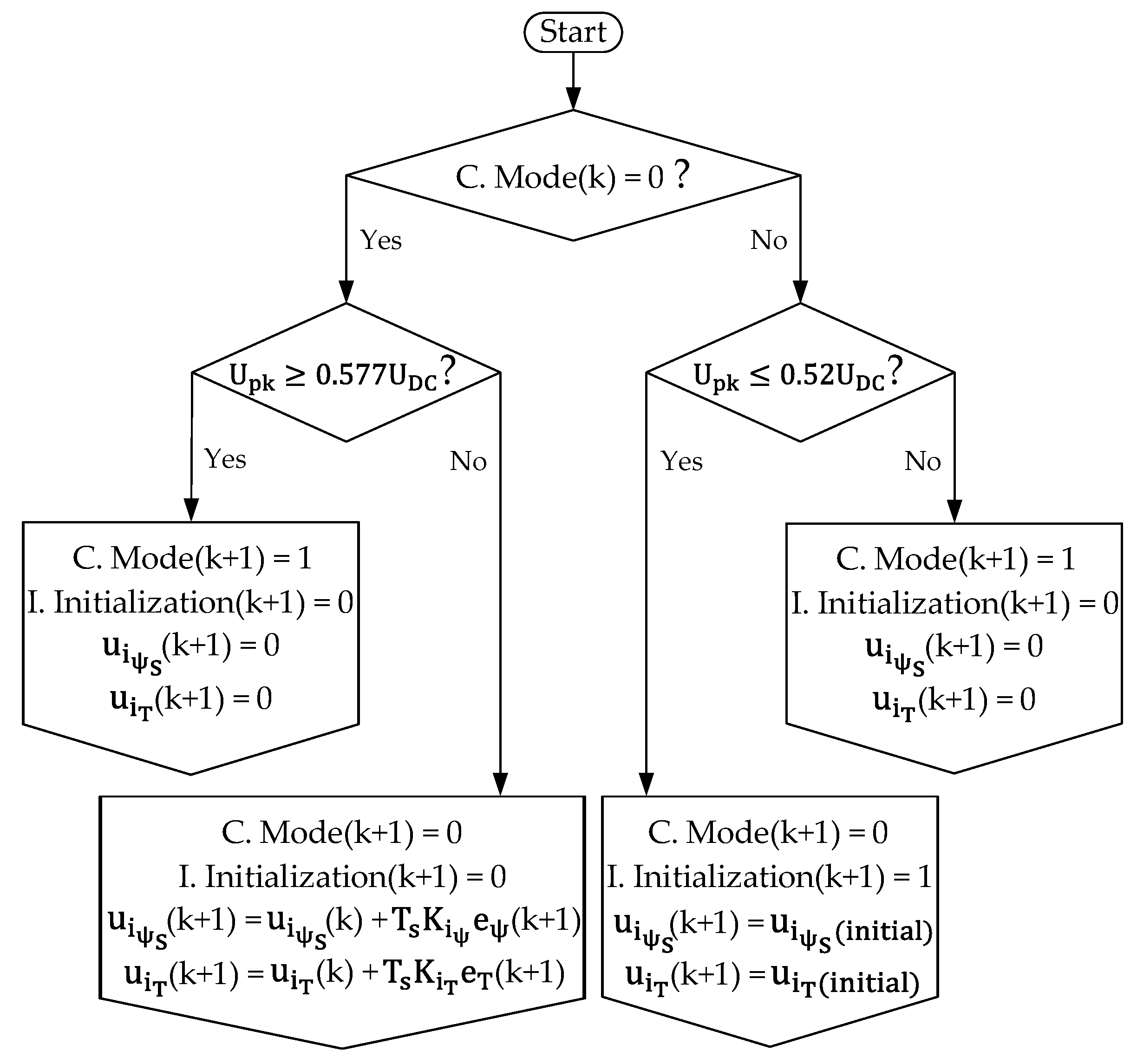
Figure 14 shows the flowchart for the control mode selection algorithm. It also includes the signal to trigger the PI integral initialization algorithm. Furthermore, for every situation, the approach that will be followed to obtain ${\mathrm{u}}_{{\mathrm{i}}_{{\mathsf{\psi }}_{\mathrm{s}}}}$ and ${\mathrm{u}}_{{\mathrm{i}}_{\mathrm{T}}}$ is also shown in the flowchart. Based on the present cycle conditions, it is decided how the control algorithm will act in the next cycle. In the flowchart, C. Mode(k + 1) = 0 means that DTC–SVM will be implemented in the next control cycle, whereas C. Mode(k + 1) = 1 means that conventional DTC will be implemented instead. I. Initialization(k + 1) = 0 means that the integral algorithm will not be triggered in the next control cycle, whereas I. Initialization(k + 1) = 1 means that the integral algorithm will be triggered instead.

Calculation of $u_{i_{{\psi }_s}\left(initial\right)}$ and $u_{i_T\left(initial\right)}$

The calculation of ${\mathrm{u}}_{{\mathrm{i}}_{{\mathsf{\psi }}_{\mathrm{s}}}\left(\mathrm{initial}\right)}$ and ${\mathrm{u}}_{{\mathrm{i}}_{\mathrm{T}}\left(\mathrm{initial}\right)}$ is performed with the following steps:

• With the stator flux-oriented scheme, $\overrightarrow{{\mathsf{\psi }}_{\mathrm{ds}}}=\overrightarrow{{\mathsf{\psi }}_{\mathrm{s}}}$ and $\overrightarrow{{\mathsf{\psi }}_{\mathrm{qs}}}=0$. Hence, the stator voltage machine equations in the $\mathrm{d}-\mathrm{q}$ frame are:

  $${\mathrm{v}}_{\mathrm{ds}}={\mathrm{R}}_{\mathrm{s}}{\mathrm{i}}_{\mathrm{ds}}+\frac{{\mathrm{d}\mathsf{\psi }}_{\mathrm{s}}}{\mathrm{dt}}$$

  (28)

  $${\mathrm{v}}_{\mathrm{qs}}={\mathrm{R}}_{\mathrm{s}}{\mathrm{i}}_{\mathrm{qs}}+{\mathsf{\omega }}_{\mathrm{s}}{\mathsf{\psi }}_{\mathrm{s}}$$

  (29)
• Assuming steady-state conditions, ${\mathrm{d}\mathsf{\psi }}_{\mathrm{s}}/\mathrm{dt}=0$ and ${\mathsf{\psi }}_{\mathrm{s}}={ \mathsf{\psi }}_{\mathrm{s}}{}^{*}.$ Additionally, as shown in Figure 5, ${\mathsf{\omega }}_{\mathrm{sl}}\approx {\mathrm{K}}_{\mathrm{Tsl}}{\mathrm{T}}^{*}$. Hence, (28) and (29) can be rewritten as follows:

  $${\mathrm{v}}_{\mathrm{ds}}={\mathrm{R}}_{\mathrm{s}}{\mathrm{i}}_{\mathrm{ds}}$$

  (30)

  $${\mathrm{v}}_{\mathrm{qs}}={\mathrm{R}}_{\mathrm{s}}{\mathrm{i}}_{\mathrm{qs}}+\left({\mathsf{\omega }}_{\mathrm{m}}+{\mathrm{K}}_{\mathrm{Tsl}}{\mathrm{T}}^{*}\right){ \mathsf{\psi }}_{\mathrm{s}}{}^{*}$$

  (31)
• As shown in Figure 12, ${\mathrm{v}}_{\mathrm{ds}}{}^{*}={\mathrm{u}}_{\mathrm{ds}}+{\mathrm{v}}_{\mathrm{ds}\left(\mathrm{comp}\right)}$. Hence, ${\mathrm{u}}_{{\mathrm{i}}_{{\mathsf{\psi }}_{\mathrm{s}}}\left(\mathrm{initial}\right)}$ is obtained by:

  $${\mathrm{u}}_{{\mathrm{i}}_{{\mathsf{\psi }}_{\mathrm{s}}}\left(\mathrm{initial}\right)}={\mathrm{R}}_{\mathrm{s}}{\mathrm{i}}_{\mathrm{ds}}-{\mathrm{K}}_{{\mathrm{P}}_{\mathsf{\psi }}}{\mathrm{e}}_{\mathsf{\psi }}-{\mathrm{v}}_{\mathrm{ds}\left(\mathrm{comp}\right)}$$

  (32)

  where ${\mathrm{K}}_{{\mathrm{P}}_{\mathsf{\psi }}}$ is the flux controller proportional constant and ${\mathrm{e}}_{\mathsf{\psi }}$ is the stator flux error.

As shown in Figure 12, ${\mathrm{v}}_{\mathrm{qs}}{}^{*}={\mathrm{u}}_{\mathrm{qs}}+{\mathrm{v}}_{\mathrm{qs}\left(\mathrm{comp}\right)}$. Hence, ${\mathrm{u}}_{{\mathrm{i}}_{\mathrm{T}}\left(\mathrm{initial}\right)}$ is obtained by:

$${\mathrm{u}}_{{\mathrm{i}}_{\mathrm{T}}\left(\mathrm{initial}\right)}={\mathrm{R}}_{\mathrm{s}}{\mathrm{i}}_{\mathrm{qs}}+\left({\mathsf{\omega }}_{\mathrm{m}}+{\mathrm{K}}_{\mathrm{Tsl}}{\mathrm{T}}^{*}\right){ \mathsf{\psi }}_{\mathrm{s}}{}^{*}-{\mathrm{K}}_{{\mathrm{P}}_{\mathrm{T}}}{\mathrm{e}}_{\mathrm{T}}-{\mathrm{v}}_{\mathrm{qs}\left(\mathrm{comp}\right)}$$

(33)

where ${\mathrm{K}}_{{\mathrm{P}}_{\mathrm{T}}}$ is the torque controller proportional constant and ${\mathrm{e}}_{\mathrm{T}}$ is the torque error.

9. Simulation and Experimental Results

To verify the performance of the proposed method, simulation and experimental measurements were performed with motor, inverter and controller parameters as presented in

Table 3. Parameters of the Induction Motor.

Parameter	Value	Parameter	Value
Rated Power	1.5 kW	Rated Torque	8.29 N·m
Rated Speed	1800 r/min	Stator Resistance	4.48 Ω
Rated Voltage	380 V	Rotor Resistance	2.78 Ω
Rated Current	3.3 A	Mutual Inductance	0.415 H
Rated Frequency	60 Hz	Stator Inductance	0.43 H
Inertia	0.017 kg·m2	Rotor Inductance	0.43 H

,

Table 4. Parameters of the Inverter.

Parameter	Value	Parameter	Value
Switching frequency	10 kHz (DTC–SVM)	Dead-time	2 µs
DC bus capacitor	1 mF	DC bus voltage	600 V

,

Table 5. Parameters of the Controllers.

		Speed Controller	Torque Controller	Flux Controller
Conventional DTC	$\mathrm{PM}$	60°	Hysteresis	Hysteresis
	${\mathsf{\omega }}_{\mathrm{c}}$	2.5 Hz
	${\mathrm{K}}_{\mathrm{p}}$	0.23
	${\mathrm{K}}_{\mathrm{i}}$	2.1
	${\mathrm{T}}_{\mathrm{S}}$	1/40,000 s	1/40,000 s	1/40,000 s
DTC–SVM	$\mathrm{PM}$	60°	55°	55°
	${\mathsf{\omega }}_{\mathrm{c}}$	2.5 Hz	300 Hz	300 Hz
	${\mathrm{K}}_{\mathrm{p}}$	0.23	21.6	1793
	${\mathrm{K}}_{\mathrm{i}}$	2.1	20,591	1,494,446
	${\mathrm{T}}_{\mathrm{S}}$	1/10,000 s	1/10,000 s	1/10,000 s

, respectively.

The controller algorithm was implemented on a TMS320F280049 (32-bit, 100 MHz) microcontroller from Texas Instruments. The DSP PWM module can be configured to generate the switching states in a PWM fashion and, also, to generate said states by forcing the output to set (high) or to clear (low). Hence, when conventional DTC is implemented, based on Table 2, the DSP is configured to force the switching states to high or low for the whole switching period. On the other hand, when DTC–SVM is implemented, the DSP is configured to generate the switching states by comparing the SVPWM control signal with the carrier. When there is change in the control mode, the DSP is programmed to switch the PWM module configuration to be ready for the next control cycle, where the new control mode starts.

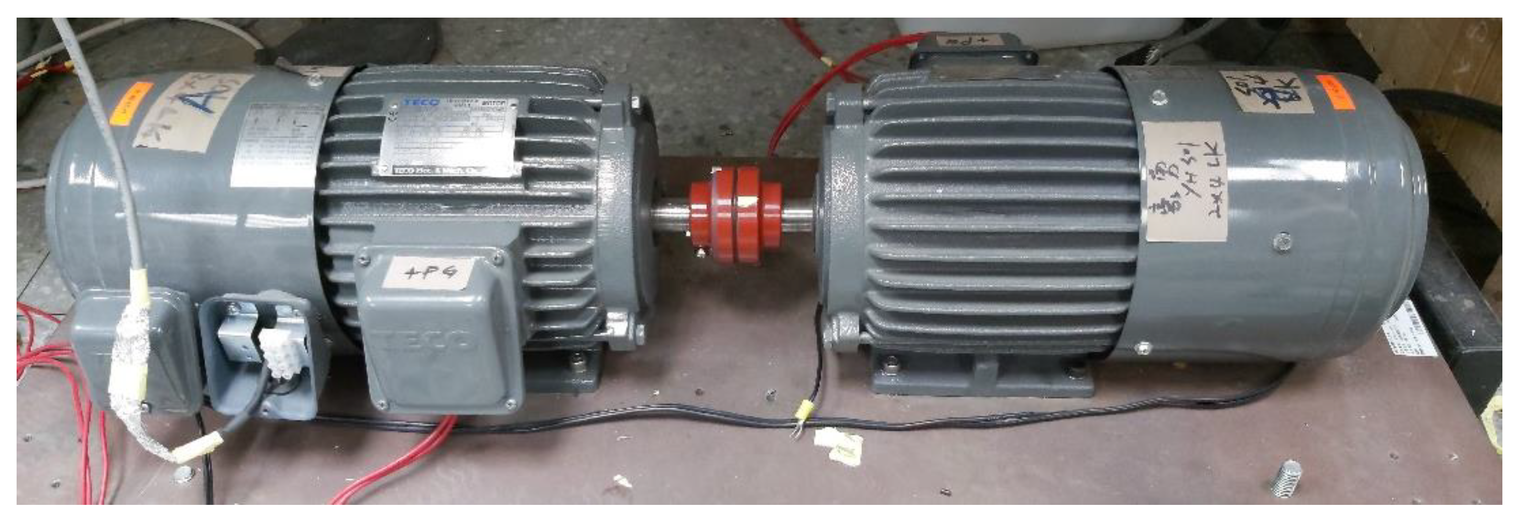
As is presented in Figure 15, two IMs are connected through a coupling. One motor is used to implement the proposed control algorithm while the other is controlled with standard FOC as a load. Three-phase currents are measured using Hall effect sensors. An incremental encoder is used to measure the rotor speed.

Simulation and experimental results are shown in every figure.

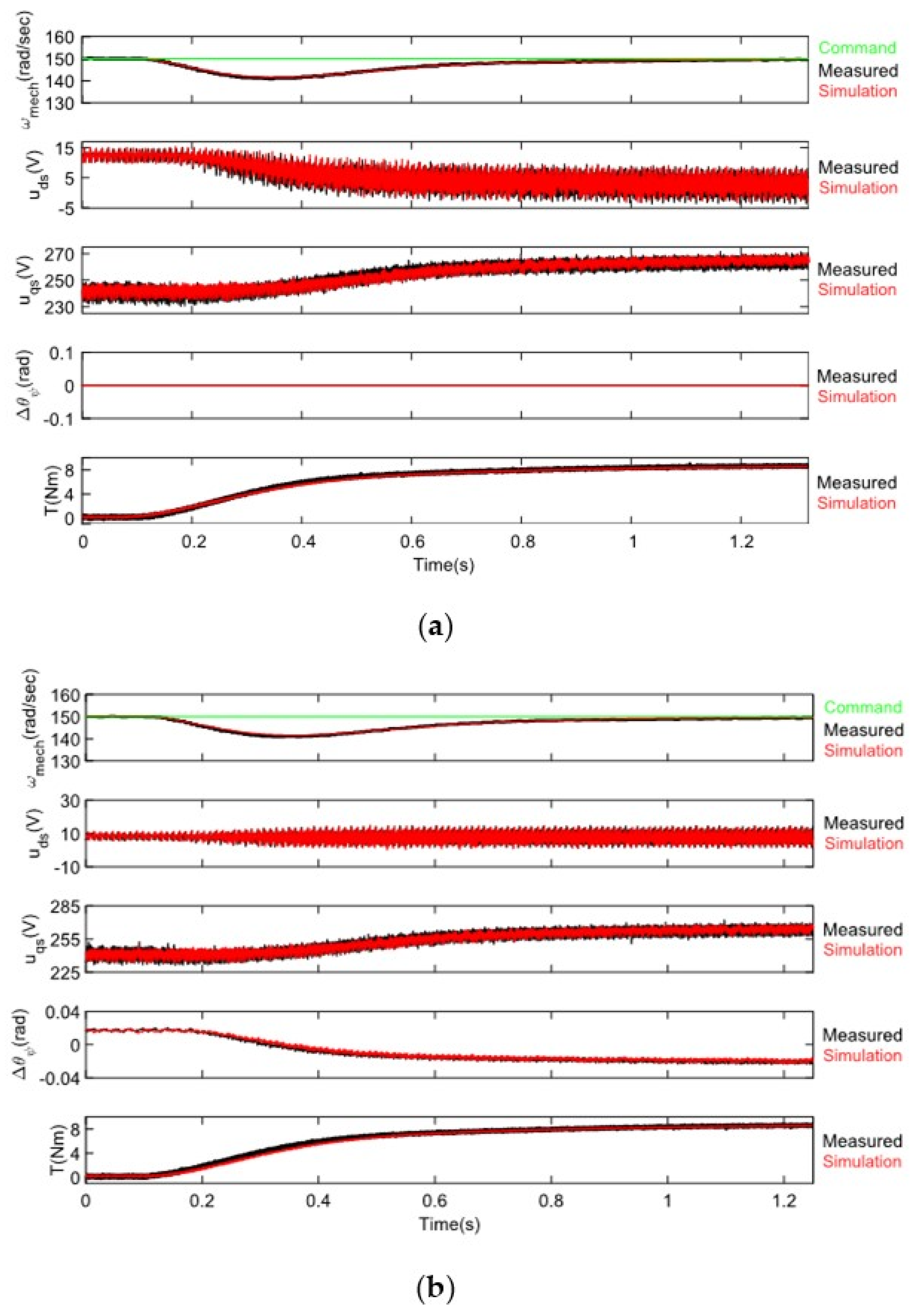
The flux and torque PI controller response without correction of ${\mathsf{\theta }}_{{\mathsf{\psi }}_{\mathrm{s}}}$ for the no-load condition is shown in Figure 16a. Figure 16b shows the same situation but with correction of ${\mathsf{\theta }}_{{\mathsf{\psi }}_{\mathrm{s}}}$.

The flux and torque PI controller response without correction of ${\mathsf{\theta }}_{{\mathsf{\psi }}_{\mathrm{s}}}$ for the rated torque condition is shown in Figure 17a. Figure 17b shows the same condition but with correction of ${\mathsf{\theta }}_{{\mathsf{\psi }}_{\mathrm{s}}}$.

The flux and torque PI controller response when ${\mathsf{\omega }}_{\mathrm{mech}}{}^{*}$ is kept constant and the load is increased from zero to its nominal value without correction of ${\mathsf{\theta }}_{{\mathsf{\psi }}_{\mathrm{s}}}$ is shown in Figure 18a. Figure 18b shows the same condition but with correction of ${\mathsf{\theta }}_{{\mathsf{\psi }}_{\mathrm{s}}}$.

As shown in Figure 16a, Figure 17a and Figure 18a, although ${\mathsf{\psi }}_{\mathrm{s}}{}^{*}$ does not change, the average value of the flux controller output $(\langle {\mathrm{u}}_{\mathrm{ds}}\rangle )$ changes. The system is behaving according to (20) instead of according to (1). Under these circumstances, the flux controller needs to adapt $\langle {\mathrm{u}}_{\mathrm{ds}}\rangle$ when ${\mathsf{\omega }}_{\mathrm{sync}}$ or $\mathrm{T}$ change. It means that torque and flux are not properly decoupled.

On the contrary, Figure 16a, Figure 17a, and Figure 18a show that when the correction on ${\mathsf{\theta }}_{{\mathsf{\psi }}_{\mathrm{s}}}$ is applied, $\langle {\mathrm{u}}_{\mathrm{ds}}\rangle$ remains practically constant, regardless if ${\mathsf{\omega }}_{\mathrm{sync}}$ or $\mathrm{T}$ change. The system is behaving according to (1) and a perfect decoupling between flux and torque is obtained.

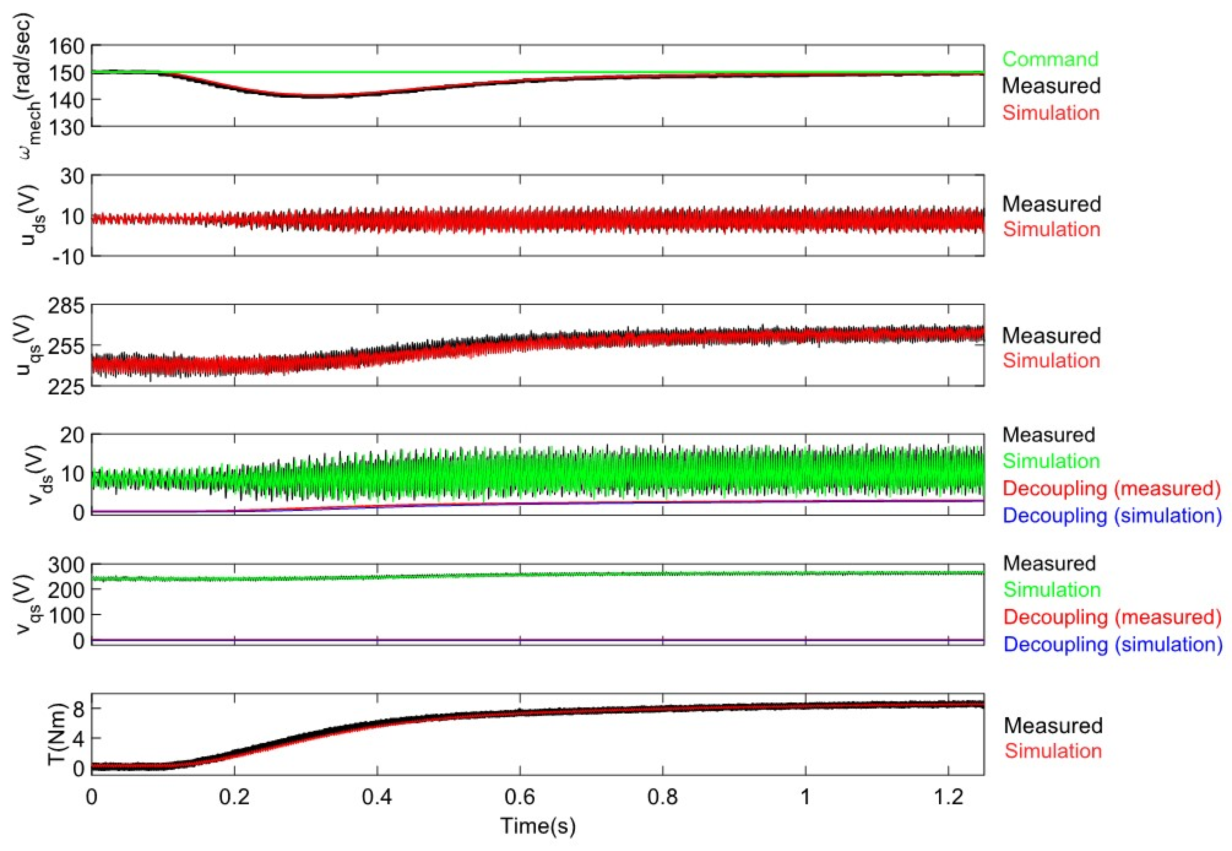
As can be observed in Figure 19, for constant ${\mathsf{\omega }}_{\mathrm{mech}}{}^{*}$, when the load changes from zero to the rated torque, the simplification for ${\mathrm{v}}_{\mathrm{ds}\left(\mathrm{comp}\right)}$ works properly. ${\mathrm{v}}_{\mathrm{ds}}{}^{*}$ achieves the desired value, while $\langle {\mathrm{u}}_{\mathrm{ds}}\rangle$ is kept constant. Regarding ${\mathrm{v}}_{\mathrm{qs}\left(\mathrm{comp}\right)}$, it is corroborated that its contribution to the torque controller is negligible. Hence, it can be removed from the control algorithm.

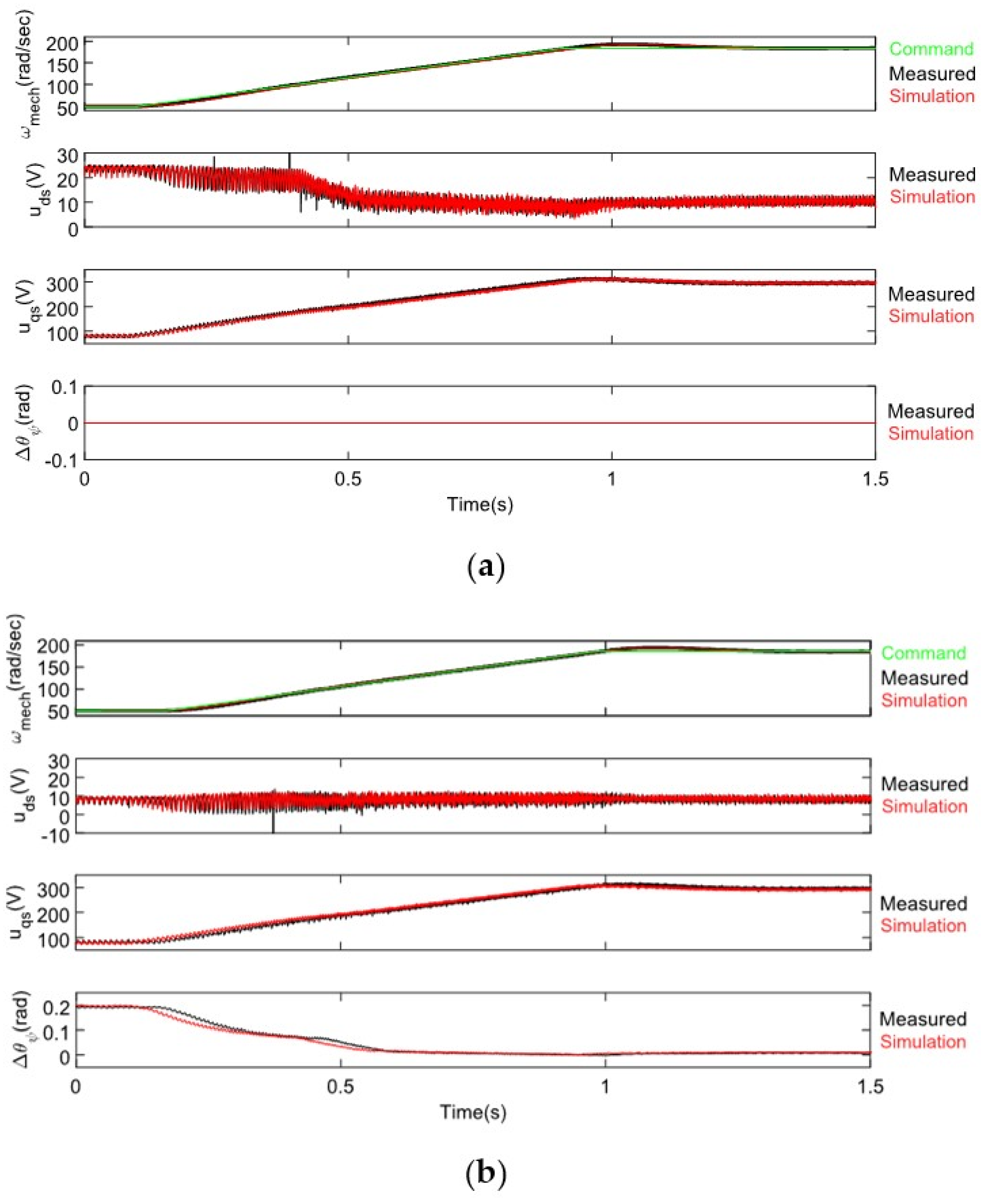
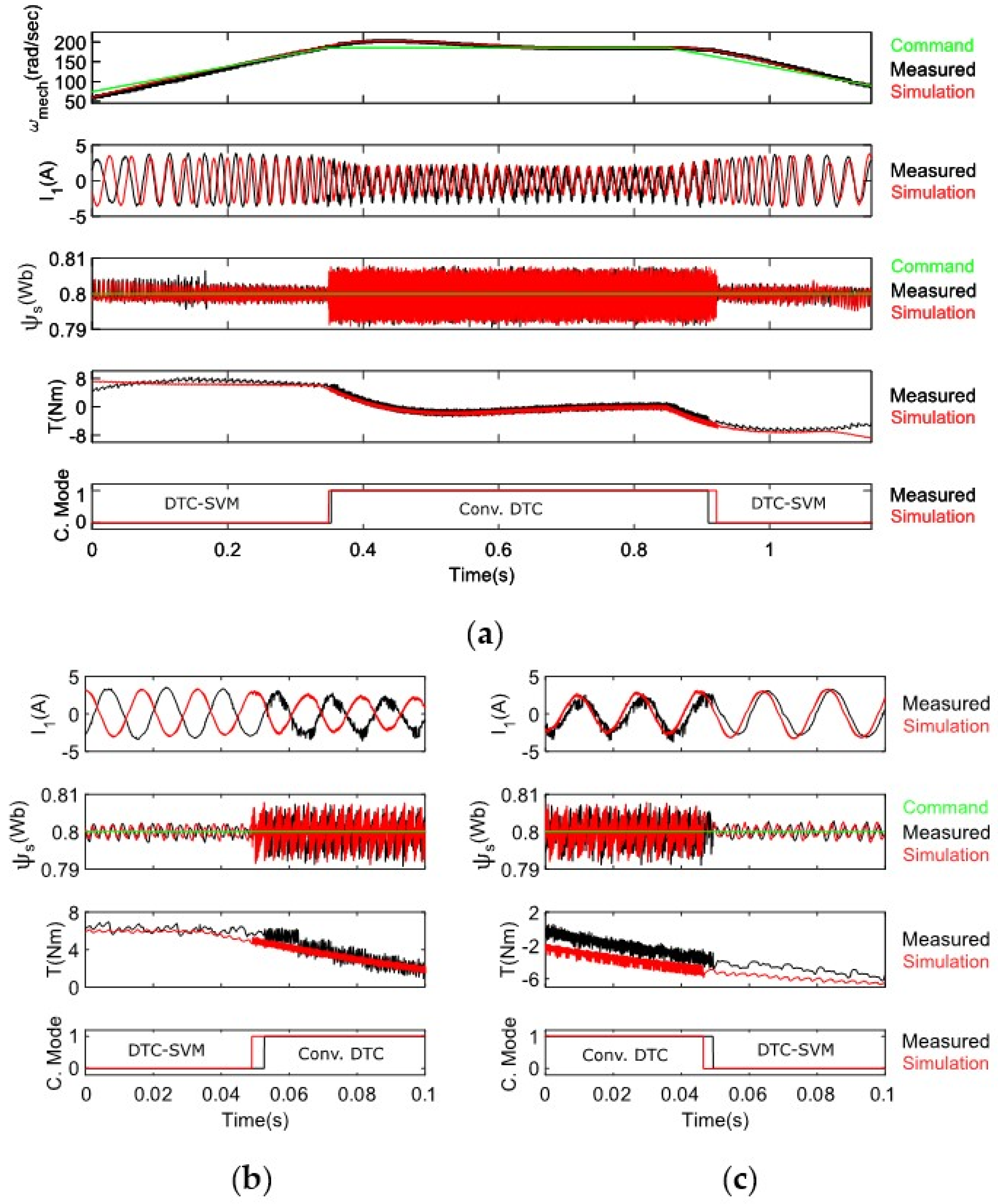
Figure 20a presents the simulation and experimental results for the acceleration and deceleration process, with its respective change in the control mode.

Figure 20b,c shows a zoom at the transition from DTC–SVM to conventional DTC and from conventional DTC to DTC–SVM, respectively. The results are shown for the no-load condition, which is the worst-case scenario owed to the higher current ripple.

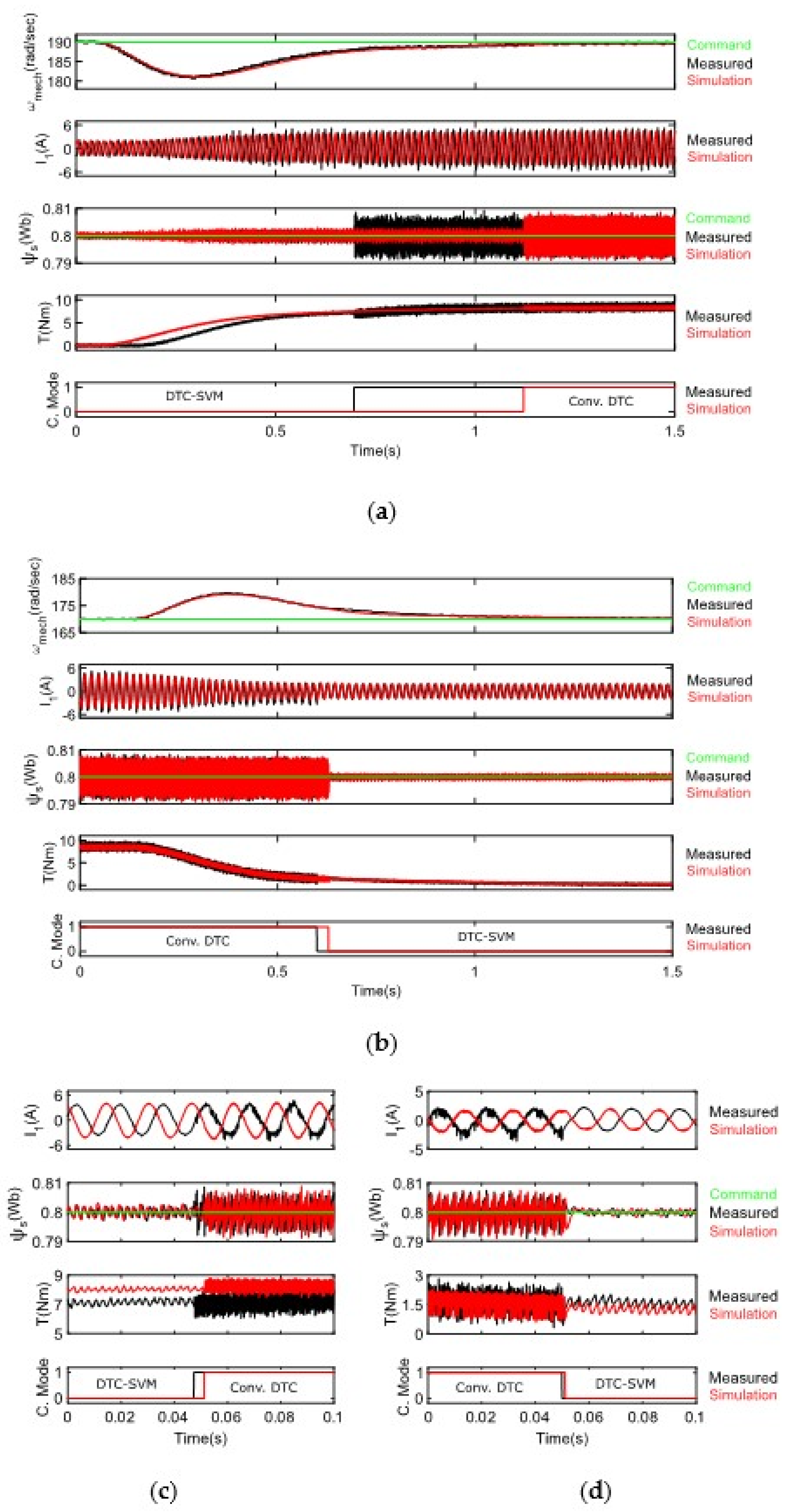
Figure 21a shows the system response when ${\mathsf{\omega }}_{\mathrm{mech}}{}^{*}$ is kept constant and the load is increased from zero to its nominal value. In order to keep the controllability of the system and provide the required phase voltage, the control mode switches from DTC–SVM to conventional DTC. Figure 21b shows the system response when ${\mathsf{\omega }}_{\mathrm{mech}}{}^{*}$ is kept constant and the load is decreased from its nominal value to zero. Since the required phase voltage is reduced to the point where DTC–SVM is enough to keep the controllability of the system, the control algorithm switches from conventional DTC to DTC–SVM. Figure 21c,d shows a zoom at the transition from DTC–SVM to conventional DTC and from conventional DTC to DTC–SVM, respectively. Due to the hysteretic approach of the control mode selection algorithm, the transition from DTC–SVM to conventional DTC takes place at a much higher current and torque than the transition from conventional DTC to DTC–SVM.

For the situation shown in Figure 20, the change in the phase voltage requirements is mainly caused by a variation on the speed. On the other hand, in Figure 21, it is mainly caused by a variation on the load.

In all situations, a smooth transition between control modes is achieved. The fundamental component of the current is not altered during the transitions. The change in the control mode is almost unnoticeable except for the fact that the current ripple is different for the two control modes.

Table 6. Measured THD (%) for DTC–SVM.

Torque (Nm)	Speed (rad/s)
	210	100	50
8	NA 1	2.34	2.01
4	NA 1	3.67	2.82
0	NA 1	4.7	3.7

¹ Conditions not attainable by this control method.

and

Table 7. Measured THD (%) for conventional DTC.

Torque (Nm)	Speed (rad/s)
	210	100	50
8	3.78	4.03 1	4.17 1
4	5.98	6.9 1	6.92 1
0	8.1	9.4 1	9.5 1

¹ With the aim of comparing both methods, the control algorithm has been forced to implement conventional DTC. Otherwise, under these conditions, DTC–SVM is implemented by the control algorithm.

summarize the measured THD for DTC–SVM and conventional DTC, respectively. Both tables show three different load and torque conditions to be compared.

Table 8. Computing time.

Control Method	Computing Time (µs)
DTC–SVM	21.2
Conventional DTC	14.9

presents the computing time needed by the DSP for DTC–SVM and conventional DTC.

Simulation and experimental results are consistent with the theoretical analysis. The good simulation and experimental results prove the feasibility and confirm the advantageous attributes of the proposed method.

10. Conclusions

A simple and robust method to maximize the DC bus utilization by exploiting the combined advantages of DTC–SVM and conventional DTC has been proposed. DTC–SVM was applied during the linear region, providing low THD, low ripple, low switching losses and constant switching frequency. Beyond the linear region, the control algorithm switched to the conventional DTC. The transition method between modes has been properly explained. Moreover, complete independence of the motor parameters was achieved in both regions. Additionally, a simplified method to decouple torque and flux, which does not require the differentiation of ${\mathrm{i}}_{\mathrm{qs}}$ has been proposed. Furthermore, a compensation strategy for stator flux angle estimation due to system nonlinearities has been also proposed in this paper.

To verify the feasibility of the proposed control scheme, experimental tests have been performed on a 1.5 kW IM inverter system. Instantaneous torque response during the whole operation region, a smooth transition between the two modes, and 100% DC bus voltage utilization were achieved using the proposed method.