Forecasting of Wind and Solar Farm Output in the Australian National Electricity Market: A Review

Abstract

Accurately forecasting the output of grid connected wind and solar systems is critical to increasing the overall penetration of renewables on the electrical network. This is especially the case in Australia, where there has been a massive increase in solar and wind farms in the last 15 years, as well as in roof top solar, both domestic and commercial. For example, in 2020, 27% of the electricity in Australia was from renewable sources, and in South Australia almost 60% was from wind and solar. In the literature, there has been extensive research reported on solar and wind resource, entailing both point and interval forecasts, but there has been much less focus on the forecasting of output from wind and solar systems. In this review, we canvass both what has been reported and also what gaps remain. In the case of the latter topic, there are numerous aspects that are not well dealt with in the literature. We have added discussion on the value of forecasts, rather than just focusing on forecast skill. Further, we present a section on how to deal with conditionally changing variance, a topic that has little focus in the literature. One other topic may be particularly important in Australia at the moment, but may become more widespread. This is how to deal with the concept of a clear sky output from a solar farm when the field is oversized compared to the inverter capacity, resulting in a plateau for the output.

1. Introduction

The goal is to describe the present state of forecasting power output from solar and wind farms. Narrowing the topic from forecasting the resource arises from the present needs of the Australian National Electricity Market (NEM) and we suggest the near future needs of markets throughout the world. In the past, and we will document some of this activity, the focus has been on forecasting the resource, solar radiation or wind speed. In [1], there is an explicit representation of what forecasting tools operate at which time and spatial scales. The depiction does not include artificial intelligence tools apart from artificial neural network (ANN) models. Our work in this review will focus mainly on the forecast horizon that is relevant to the NEM. The way the NEM works is that there are three types of generators. Scheduled generators submit a bid stack every five minutes throughout the year detailing how much electricity they can supply in the subsequent five minutes at each of ten price bands from −$AUD1000$ to $AUD\mathrm{15,000}$ per MWh. They are termed price makers. Renewable energy generators with capacity between 30 and 100 MW are termed semi-scheduled generators. They do not submit bids, but can be curtailed. Generators of any type under 30 MW are non scheduled and cannot be curtailed. The latter two categories are termed price takers, and they cannot affect the market. After the scheduled generators submit their bid stacks, the Australian Energy Market Operator (AEMO) runs a linear program to determine how far up the stack they have to go to meet their forecasted electricity demand. This is then the spot price and all generation in that five-minute period is paid that price.

In 2014, AEMO established the Australian Solar Energy Forecasting System (ASEFS), a derivative of the Australian Wind Energy Forecasting System (AWEFS) that it established years before in response to the growth in wind farm development in Australia, beginning in the early 2000s. The AWEFS was somewhat derived from similar systems at play in Europe, but with modifications to suit the NEM. It combines SCADA (Supervisory Control and Data Acquisition) measurements from the farm with Numerical Weather Prediction (NWP) forecasts as well as information about the operating condition of the farms, such as turbines out of action and so on to produce forecasts at various time scales and horizons, including the five-minute operational forecast period. The ASEFS system was developed to provide similar activities for solar farms above 30 MW capacity. For a five-minute ahead timeframe, ASEFS produces Unconstrained Intermittent Generation Forecasts (UIGF), which are used to produce a dispatch target for the semi-scheduled solar farm. Failing to come within a prescribed tolerance of that target can result in what is termed a Causer Pays penalty. From AEMO, contribution factors are determined for the purpose of assigning the costs of regulating Frequency Control and Ancillary Services (FCAS) to those market participants who have caused the need for those services. Because the penalties were becoming onerous for wind and solar farms, AEMO decided in 2018 that by the end of 2020, these generators would have to self forecast their output before the start of a five-minute interval for that interval. In reality, the goal is to forecast the power output for time t at approximately seven minute before, in order to give time to relay the forecast to AEMO and for that body to react.

In order to manage the transition, AEMO asked the Australian Renewable Energy Agency (ARENA) to fund projects to help the wind and solar farms improve their forecast capabilities. Two of the authors (Boland and Farah), were part of one of the funded projects, the Solar Power Ensemble Forecaster (SPEF). This team blended forecasts from statistical, NWP, sky camera and satellite tools. We mention this as one example of how the field of forecasting is advancing. However, the main point to make is that in Australia, as in the rest of the world, the need for reliable forecasting of solar irradiance and also output from solar farms is increasing.

In this paper, we will go into some detail about the point forecasting of wind speed and wind farm output, plus solar irradiance and solar farm output, as well as interval forecasting. We will also describe what is being done about another growing problem in this field, that of forecasting ramps. Ramps are sudden changes in output caused principally by cloud motion. Obviously these ramps may be sudden negative or positive changes. Finally, we will describe a number of areas that are not covered, or inadequately covered in the literature. As one example, the solar farms in Australia generally have oversized fields of panels. We suggest this is probably to have a better idea of the projected output for a number of hours on a clear day. As a result, the concept of a clear sky model for solar irradiance must be adjusted for the farm output. We suggest that these gaps result principally from the fact that dealing with output from large scale solar installations distributed throughout the grid is a relatively recent phenomenon.

2. Forecasting Methods

In [2], there are a number of articles referred to that deal with various point forecasting methods. These are summarised in

Table 1. Point forecasting.

Forecast Model	Evaluation Metrics (Best Results)	Reference
Elmann artificial neural network	NMBE (−0.21%), NMAE (6.50%), SD (0.11%), NRMSE (10.91%)	De Giorgi et al. [4]
Regressions in logs, autoregressive integrated moving average (ARIMA), unobserved components models, transfer functions, neural networks and hybrid models	MAPE (0.1263)	Reikard [5]
Multiple feed-forward neural networks for irradiance forecast + PV model	MAE (7.03 W/m2), MAPE (3.41%), RMSE (8.60 W/m2), R (0.99)	Durrani et al. [6]
Least square support vector machines (LS-SVM), LS-SVM with wavelet decomposition, ANN	NMBE (0.12%), NMAE (6.40%), NRMSE (9.60%)	De Giorgi et al. [7]
Correlation-based feature selection for univariate and multivariate NN ensemble and SVR	MAE (45.11 kW), MRE (3.92%)	Rana et al. [8]
Feed-forward neural networks and physical hybrid ANN	NMAE (<1.0%), WMAE (1.96%)	Nespoli et al. [9]
Fourier series with coupled autoregressive (AR) and dynamical system (CARDS) model	MeAPE (7.53%, 10.85%), MBE (0.45, 0.0002), KSI (17.92%, –), NRMSE (16.50%, 17.16%)	Huang et al. [10], Huang and Boland [11]
Autoregressive moving average (ARMA) and ARIMA models fitted by the log-likelihood function	MAE (37.95 W/m2), MAPE (0.1%)	Colak et al. [12]
Fourier series plus autoregressive models, clear sky index plus plus neural net models and clear sky index plus ARMA models	NMBE (0.08%), NRMSE (10.91%), NMAD (5.12%)	Boland et al. [13]
Global and mesoscale numerical weather prediction models combined with persistence model, time series models, k-nearest neighbours (KNN) models, ANN models and adaptive neuro-fuzzy models	RMSE (4243.01 Wh), NRMSE (11.79%), ME (−42.8 Wh), NME(−0.12%), MAE (2308.3 Wh), NMAE (6.41%)	Fernandez-Jimenez et al. [14]
Reforcasting model combined with cloud tracking, ARMA and KNN models	MBE (0.1 kW), MAE (20.7 kW), RMSE (35.5 kW), SRMSE (26.2%)	Chu et al. [15]
Verification of deterministic forecasts	A review paper	Yang et al. [16]

. In [3], a similar array of papers was described for interval or probabilistic forecasting, as in

Table 2. Interval forecasting.

Forecast Model	Reference
Non-parametric predictive density of solar irradiance for probabilistic forecasting	Grantham et al. [17]
Probabilistic forecasting of solar radiation	Grantham et al. [17]
Probabilistic forecasting of PV power	Ni et al. [18]
Probabilistic forecasting of solar radiation	Boland and Grantham [19]
Probabilistic forecasting of solar radiation	Golestaneh et al. [20]
Ensemble solar forecasting with probabilistic post processing	Yagli et al. [21]
ARMA and GARCH for prediction intervals	David et al. [22]
Review of tools for probabilistic forecasting of PV power	Ahmed et al. [23]
Review of tools for probabilistic forecasting of wind power generation	Zhang et al. [24]
Probabilistic forecasting of wind power generation using predictive distribution optimisation	Sun et al. [25]
Probabilistic forecasting of wind power generation using Gaussian mixture models	Jin et al. [26]
Probabilistic forecasting of wind power generation using ensemble methods	Kim and Hur [27]

. We include error measures for the tools in the papers in Table 1. For probabilistic forecasting tools in Table 2, there is little agreement in the field as yet as to what measures are appropriate for evaluating methods. However, it is hoped that this will be rectified in the near future through a project in Task 16 of the International Energy Agency. This project focuses on the benchmarking of probabilistic forecasting methods and is led by Professor Philippe Lauret of Université de La Reunion, and includes present author Boland.

As can be seen from Table 1, methods for point forecasting vary enormously. They range from very straightforward structural models through NWP, satellite tools to artificial intelligence methods. Also what varies is both the scale and forecasting horizon, and that also has impact on what type of model is used. In [1], their Figure 4 gives a good description of the temporal and spatial zones for different approaches. The methods for probabilistic forecasting of wind and solar energy are varied. They range from use of ensemble methods, particularly for wind speed, to parametric methods using assumptions that the error distributions are either Gaussian, Laplace or other, to non-parametric methods such as quantile regression. We will now give greater detail on a few papers that give us insight into the range of techniques.

3. Point Forecasting

Jiang et al. [28] use a combination of long short-term memory (LSTM) and autoregressive moving average (ARMA) approaches for forecasting five-minute power with a zero lead time. The training set and test set were randomly selected from the PV microgrid system of Hangzhou Dianzi University and used for PV output prediction according to different seasons and weather types. The results for the combined LSTM-ARMA compared well with either single model and also against a persistence forecast. The evaluations were performed for a small set of clear, cloudy and rainy days separately. It is good to show the results for different types of days. However, there are limitations on the study. The evaluation should be carried out on a much larger data set. Further, it would be useful to compare the results against smart persistence, rather than simple persistence. The evaluation did not include bias either, which we view as a critical measure. If a model is biased, then it should be investigated to correct this, before any other evaluation is performed. The authors also mention prediction of volatility but there is no evidence of probabilistic forecasting. Note that they also use zero lead time for the forecasts. In a scientific sense, this may be fine, but in an operational sense it is unrealistic as the grid operators need time to react to the forecast.

Mellit et al. [29] provide an extensive review of what has been published in the field of forecasting photovoltaic output power. The methods range over physical, statistical, machine learning and combinations of these. They cover both point and probabilistic forecasting tools, and discuss forecast horizons and lead times. There are a few questions that arise first. One is that it is unclear how many of the papers canvassed are actually for power from installations, and how many are for forecasting solar irradiance—for there seem to be a lot that focus on the latter. The real strength of their review is in its concluding remarks. To summarise, they point out that

• Though machine learning techniques are used a lot (note that they include ANN as an ML technique), deep learning techniques have not been utilised as much.
• Very short term, very long term and regional forecasting are subjects that are not covered well.
• Most artificial intelligence (AI) methods work well on sunny days but poorly on cloudy ones.
• Hybrid models work best.

Chen et al. [30] predict one-step-ahead five-minute power output of solar PV systems with long short-term memory (LSTM) models learned from historical power outputs and meteorological measurements (temperature, relative humidity, global horizontal radiation and diffuse horizontal radiation). Notably, they train individual LSTM models with varied data set at each forecasting time step. Hence, a radiation classification coordinate (RCC) method is proposed to select the training samples as the most similar time points in the past 30 days based on the lagged global horizontal radiation profile approaching the time points. The proposed RCC-LSTM model achieved higher forecast accuracy than four other data-driven models of the test results over 12 random days (3 days each for four seasons). However, the testing sample size is too small when two years of data are available. Moreover, the RCC-LSTM model seems to have a lagging issue in addressing sudden ramps, as seen in their Figure 10. It is worth mentioning that, unlike solar farms in Australia, the two solar systems studied do not oversize the field of panels compared to their inverter capacity. A significant observation they make is that the choice of prediction model often depends on the application scenario. We suggest that this is a very important observation and we will examine this connection of model and purpose further in Section 7.2.

In their work [31], Al Kandari and Ahmad explore four averaging approaches (from simple to weighted) to combine machine learning and statistical models and achieved higher accuracy in forecasting day-ahead daily solar PV power generation from historical meteorological data and solar power output. The proposed machine learning and statistical hybrid model (MLSHM) consists of the long short-term memory (LSTM) model, the gated recurrent unit (GRU) model and the Theta statistical method. To increase the diversity of the proposed ensemble model, the authors train the two machine learning models with separate datasets. However, it is unclear whether the training datasets are representative of the overall dynamics of the application data. Furthermore, the window size for LSTM and GRU is set to 2 in the experiments, meaning the forecast is learned from the previous two days data. Therefore, it suggests the LSTM or GRU may not be the best option if there is no long-term relationship in the time series of the normalised daily solar power output. It would also be good to explore and verify the importance of meteorological data in their study. Moreover, additional coefficients are recommended for the Theta statistical model to fit the Cocoa data where large variability exists.

Delgado and Fahim [32] analyse the ten-minute SCADA system data of wind turbines to understand the wind behaviour and power generation patterns with three proposed visualisations: Cartesian, polar, and cylindrical coordinates. They also present univariate one-step-ahead forecasting models based on long short-term memory (LSTM), covering both resource (wind speed and direction) and power output (generated active power and derived theoretical power). The test results show the predictions match actuals with minor errors except for time steps of abrupt changes. Notably, higher accuracy is achieved in forecasting wind speed than active power generation. The one proviso to this is that the error metrics are not normalised so it is hard to tell how good the performance is compared to other approaches. If instead there was a comparison to a commonly used benchmark, it would be easier to make a judgement of the worth.

Ibrahim et al. [33] attempt to predict next-step intra-hour wind speed uncertainties from lagged time series data by fitting different machine learning techniques, from ANN, CNN to LSTM and SVM. They proposed a hybrid convolutional LSTM (ConvLSTM) model for high accuracy and low computation cost. However, all studied models have comparable forecasting accuracies under individual optimum settings and perform better at 5 min time resolution than 30 min or 1 h.

4. Interval Forecasting

Wang et al. [34] use a combination of wavelet transform, deep convolutional neural network and quantile regression for deterministic and probabilistic photovoltaic power forecasting. In this case, they perform the analysis on actual solar farm data from two farms in northern Belgium. They work on a 15 min time scale, and forecast variously for 30, 45 and 75 min ahead, calibrating the models on a monthly basis to cater for seasonality. It appears the deterministic models perform well but they do not use a standard benchmark for comparison. They use what they call interval sharpness, but which is usually termed interval score, to evaluate the performance of the probabilistic forecasting, along with coverage. Once again the model appears to perform well.

Alessandrini et al. [35] uses what they call an Analog Ensemble (AnEn) for solar power forecasting. What this means is that when presented with a particular set of characteristics of a present forecast situation, a search is performed to identify what the next forecast step’s output was for a situation in the past that most closely resembles the present one, and that output is used for the forecast. They use solar farms near Milan in northern and Catania in southern Italy for testing. The ensemble idea is that they choose a small number, often three possible close forecasts and use them as an ensemble. They then compare this probabilistic forecast with what they would obtain with quantile regression. In essence the various methods perform similarly, with perhaps a slight leaning towards AnEn. The point they make, and in our opinion it is a valid one, is that it is beneficial that all the methods they use do not need a irradiance to power conversion—all the modelling is performed using past output from the solar farms.

Van der Meer et al. [36] discuss probabilistic forecasting for photovoltaic power, electricity demand of a sector and also of an individual dwelling. They use Gaussian Processes to perform the probabilistic forecasting estimates. It would seem that the results, in their view, are fine since if trying for an $80\%$ prediction interval, they obtain between 82 and $91\%$. However, if one is trying for $80\%$, then the results should actually be close to $80\%$ in all instances. Perhaps this is because they have not considered the fact that the distributions they are dealing with are far from Gaussian. Further, they may be not considering the serial correlation of the variance in this type of forecasting.

Even though this research is almost a decade old, Pinson [37] provides one of the most precise descriptions of the differences in forecasting output from a wind (or indeed solar) farm versus forecasting the resource. There is the salient point made that the characteristics of wind power are the motivation for the choice of specific types of predictive distributions. The wind power is bounded below by zero and above by the capacity of the farm—$P_n$. It is the same for a solar farm. There is one proviso in Australian wind and solar farms—the lower bound is slightly below zero, to cater for the power drawn from the grid to run the control systems when there is no resource input. In that paper, they then normalise the output by dividing by $P_n$. They go on to say that the output is related to the wind speed by a sigmoid curve and the resulting distribution of output is not Gaussian, so any predictive interval estimation must take that into account. In their words, predictive densities take the form of discrete continuous mixtures consisting of a generalised logit-Normal (GL-Normal) distribution with potential concentration of probability mass at the bounds of the unit interval [0, 1]. In their approach, they prescribe a shape parameter for these densities and they then are characterised only by a location and scale parameter. So, they can perform a generalised logit transform and then they can model the resultant with a censored Gaussian distribution. In some ways, it may seem a complicated procedure, but it reflects the reality of the situation in dealing with a situation that is far from the desired simple time series structure, as in Equation (1).

Any additive one step ahead statistical forecasting method can be encapsulated by the structure

$$Y_t=f(S_t;R_{t-1},\dots ,R_{t-p})+a_t$$

(1)

where $R_t=Y_t-S_t$, and $S_t$ denotes the representation of the seasonality. Knowledge of the statistical qualities of $a_t$ is necessary in order to construct the error bounds of the forecast. In this formulation, the hope is that the noise is independent and identically distributed, and in the best situation, follows a Gaussian distribution. As discussed above, the output from wind farms, and also solar farms, contravenes the Gaussian assumption. Additionally, it will be shown explicitly that the output from either wind or solar farms is dependent, in that the variance possesses an autocorrelative effect. In [37], they employ a form of dynamics in their model approach, but as they point out, they do not cater for conditional heteroscedasticity—dynamically changing variance. We will describe in Section 7.3 how one can deal with this effect—the autoregressive conditional heteroscedastic (ARCH) phenomenon, as more fully described in [3]. In summary, this paper is reflective of thought on this topic that has only become accepted years after its publication.

Tahmasebifar et al. [38] propose a three stage hybrid model for forecasting one hour and one day ahead for Australian wind farms. To give a short description, they combine extreme learning machine (ELM), wavelet transforms, bootstrapping, ensemble forecasting and particle swarm optimisation. The results look very good, but there are a number of problems. One is that they are not dealing with the requirements for forecasting for the Australian NEM, in that forecasts have to be made on a five minute time scale, with a forecast lead time of approximately seven minutes, for the instantaneous power. So, it is not possible to compare results to those in a recent trial by the AEMO. Further, the method is very complicated and it is difficult to decipher what segments are generating particular benefits.

5. Ramp Forecasting

From a particular viewpoint, including potentially from a financial perspective, advance knowledge of a significant change in the output of a wind or solar farm, is more important than an estimate of the absolute output. Taylor [39] develops a method for forecasting ramp events and applies it to four wind farms in Crete. The author talks of probabilistic forecasting of a ramp event, but uses that term in a different manner from what it usually means in this field. What he refers to as probabilistic forecasting means forecasting the probability of a ramp being greater (or less than) a specific threshold. He predicts the probability of a ramp event in wind power for one and two steps ahead by fitting autoregressive logit based models to lagged hourly wind power changes. The author first forecasts ramping probability in the next step for a single ramping threshold and a single wind farm then introduces three conditional autoregressive multinomial logit (CARML) models in jointly estimating probabilities for multiple thresholds, two wind farms and two steps ahead, respectively. All models are optimised by maximising the likelihood of variant Bernoulli distributions. The Brier skill score demonstrates the superiority of the proposed models against selected benchmarks. However, the predicted probabilities for true ramp events are not presented to show the model’s effectiveness in practice. Interestingly, jointly forecasting the probabilities of one and two steps ahead enhances one step ahead estimation in this study, which is worth exploring more. Another interesting observation is that the model could be adapted to a different definition of a ramp, such as a large change in output between non-successive time intervals.

Abuela and Chowdhury [40] use a hierarchy of models to deal with the need to mitigate the effects of difficult to predict ramps in solar farm output. One is a post-processing method where they

• Start with 24 h ahead forecasts that combine NWP forecasts with hour ahead forecasts.
• Add persistence forecasts and use the random forecast procedure to produce better forecasts.
• Add in the ramp rate, which is the forecast for the present hour minus the actual for the previous hour.
• Use a random forecast technique on this augmented set of forecasts.

In summary, they attempted to predict ramp events of rooftop solar power change at one-hour intervals as of four categories: up or down, high or low for a given threshold. The authors argue that combining forecasts from different methods, if not properly modelled, could reduce the accuracy for ramp event forecasting of solar power outputs resulting from the smoothing effect. To tackle this issue, they deployed an ensemble learning (Random Forest) model trained using a selective list of numerical weather prediction (NWP) variables, solar power forecasts and associated ramp rates deemed as the most effective features with two loss functions (one to minimise the solar power forecast errors and the other to minimise the residuals of the predicted ramp rates). Jointly optimising two losses is utilised to mitigate the lower forecasting accuracy of less frequent high ramping events, a typical problem for fitting unbalanced data. In addition, probabilistic forecasts of solar power ramps are provided based on the proposed ensemble model, and the uncertainty analysis demonstrates a lower certainty of forecasting ramp events at a higher threshold, promoting future research directions.

Probst and Minchala [41] present an interesting way to deal with ramping with wind farms. It seems to be an innovative way to deal with ramping and eminently suitable to use in increasing the value of forecasting. The idea is that with better wind power forecasts, one can plan curtailment to suit the generator, rather than have it forced upon them. The crux of the value proposition is that for a low decrease in the value of energy delivered, one can curtail the output when anticipating a large ramping event that would incur penalties for sending the frequency out of bounds. They proposed a low-cost forecast-based curtailment (FBC) approach mitigating significant downward ramps of short term wind power output to meet grid operation limits. The FBC strategy applies curtailment for the next step to reduce incompliant ramp-down events in the second step based on two steps ahead forecasts. As a result, by implementing the Kalman filtering algorithm with upstream wind measurements, about 40% of incompliance negative ramps are mitigated with negligible energy loss due to curtailments. In addition, the authors argue that mitigation efficiency can be increased from forecasting methods having a smaller correlation between wind power changes and forecast errors. In the Australian context the penalties are termed Causer Pays. One can easily view an extension to this to a situation where a wind or solar farm operator can decide when it is good to bypass curtailment, and put the output into a battery that is connected to the farm, and then use the stored energy for arbitrage. The limitation on this research is that it is developed on wind speeds, rather than wind farm output, with the extra step being a power conversion model. However, the philosophical nugget is key to the value. The next refinement is to add the extra benefit of probabilistic forecasting to this paradigm.

Han et al. [42] describe methods to improve the forecasting of ramp events for wind farms. The first step is to identify features of ramp events so that when these features occur, one has a better chance of forecasting the ramp. They use a combination of two deep learning algorithms, convolutional neural network and long short-term memory to learn the ramp features of wind power and from that be able to better forecast ramp events.

The Australian Energy Market Operator (2020) Renewable Integration Study (RIS) [43] gives a lot of detail about the comparison of point forecast and ramp forecast accuracy when discussing managing variability and uncertainty. First, they give some insight into ramp events in general. The magnitude and frequency of ramp events in the NEM are increasing, and this is due mainly to increases in variable renewable generation. The increase in ramp events indicates that some measures are needed to maintain stable operation of the grid. One major way to do this is happening with greater frequency control via super capacitors as well as the installation of storage mechanisms in the grid. However, the need for improvements in forecasting, particularly the forecasting of ramp events, is evident. As an example of the problem, the RIS shows that as the forecast lead time approaches real time, the accuracy of point forecasts increases but the accuracy of ramp forecasts does not. Obviously this leads to a significant future direction for research.

6. Synthetic Solar Time Series

Though the generation of synthetic time series of solar irradiation is not specifically forecasting, the tools that have to be developed are in the same realm. There is a long history of the development of tools for generating synthetic solar time series. Brinkworth [44] had a goal to develop synthetic sequences of solar irradiation in order to understand the potential output from solar devices. He stated that Among the important features of these variations is their sequential character, which has not hitherto been taken into account. It is shown that the sequential characteristics of the daily insolation can be represented in simple numerical terms, derived from the autocorrelation functions of a straightforward stochastic model. Since he was working with estimation of the macroscopic performance of solar systems, he concentrated on daily totals of solar irradiation. The goal was to generate sequences that matched the long term statistical characteristics, both in autocorrelation and also the moments of the distribution. In this way, one can generate sequences that could well have happened but not necessarily are in the historical record. This can lead to the design of systems that are more robust in their performance.

In the mid to late 1980s, there were a few more papers on this topic. Balouktsis and Tsalides [45] worked with hourly solar irradiation data and first dealt with the seasonality by using a Fourier series model containing terms for the annual and daily cycles. It is interesting that even though they published the paper in 1986 in Solar Energy journal, they did not refer to Phillips (1984) [46] in the same journal, who used a more rigorous investigation to determine that 75 Fourier coefficients needed to be used. Note that one of the present authors—Boland, in [47], delineated which frequencies are significant and gave physical interpretations. Balouktsis and Tsalides then went on to note that when dealing with the data that have the seasonality removed, it is important for synthetic generation to understand the characteristics of the frequency distribution of the data. If one is simply wanting to determine the autocorrelative features of the data in order to estimate an ARMA model and then use that plus the seasonal components for point forecasting, it is possible to ignore the distributional characteristics. However, if one’s intention is probabilistic forecasting or synthetic generation, more work is to be done. Let us focus here on what happens for synthetic generation. Let us assume, for example that the model for the solar irradiation is of the form

$$I_t=S_t+{\alpha }_1{R}_{t-1}+{\alpha }_2{R}_{t-2}+{\alpha }_3{R}_{t-3}+a_t$$

(2)

Here, $I_t$ is the solar irradiation, $S_t$ is the seasonal component and $R_t=I_t-S_t$. The standard method to generate synthetic data would be collect all the $a_t$ from the set that was used to estimate the model for $R_t$ and use that noise distribution in the calculations. One selects at random four values from that distribution and then finds the value for $R_4$ as

$$R_4={\alpha }_1{a}_3+{\alpha }_2{a}_2+{\alpha }_3{a}_1+a_4.$$

(3)

After that, progressively, one calculates for as many terms as required.

$$R_j={\alpha }_1{R}_{j-1}+{\alpha }_2{R}_{j-2}+{\alpha }_3{R}_{j-3}+a_j.$$

(4)

The problem is that if this is performed, the distribution of the $R_t$ will be symmetric and close to normal, even if the original distribution was skewed. To overcome this problem, they perform a normalising transformation of the data after the seasonality is removed and then construct the model with this normalised data. They refer to [48] who did this type of transformation as well. The other important component that they recognised was that the irradiation distributions change over time. They only catered for changes in distribution on a monthly basis, unlike [3], but it was innovative for the time.

The articles by Aguiar and Collares-Pereira (with Conde in one) [49,50,51] were instructive in the derivation of tools for synthetic generation. In [49], the goal was to use mean monthly solar irradiation as an input to generate synthetic sequences of daily solar irradiation. This is as an aid for long term performance evaluation of solar systems. The model relies on two assumptions. One is that there is significant correlation only between consecutive days, rather than including any more lags, after removal of the seasonal component. They canvass three methods of dealing with the seasonality. One is to construct the clearness index for the daily values. The clearness index is the global horizontal irradiation (GHI) divided by the extraterrestrial irradiation—the irradiation at the top of the atmosphere for that same day and location. The second is by subtraction from the Fourier series representation for that day. The third is by subtraction of the moving average centred on that day from the day’s irradiation. They chose the first method. The other principle they relied on is that the probability of occurrence of irradiation values is the same for months with the same mean clearness index. They then construct a library of Markov transition matrices (MTM) for clearness index, one matrix for each month. They can then employ these matrices, picking for a location the MTM from their library that has a mean monthly clearness index most closely matches the mean monthly clearness index for that location. We illustrate the procedure for using an MTM for generating synthetic sequences, by describing it with a simplified example.

Suppose we have a three state Markov chain for daily total solar irradiation. We will illustrate this for a single month to avoid having to deal with seasonality. Let us focus on Adelaide, South Australia in January and define the three states as

• State 1—1–21 MJ/m². Class Mark 10.
• State 2—21–30 MJ/m². Class Mark 25.
• State 3—30–35 MJ/m². Class Mark 33.

The Markov transition matrix is thus $\left(\begin{array}{ccc}0.97& 0.03& 0\\ 0& 0.94& 0.06\\ 0& 0.05& 0.95\end{array}\right)$

Note that the equilibrium vector, the long term probabilities of being in each state is given by $\left(\begin{array}{ccc}0.05& 0.42& 0.53\end{array}\right)$

What the transition matrix indicates is that in January in Adelaide there is a high probability of successive days being in the same solar state. To understand how this matrix can be used to generate a synthetic sequence, we can follow this path.

• Select a random number r in $(0,1)$ using a random number generator.
• If $r1<0.05$, then the initial state is 1 and the initial solar irradiation value is 10 MJ/m².
• If $r1<0.47$, then the initial state is 2 and the initial solar irradiation value is 25 MJ/m².
• Otherwise, the initial state is 3 and the initial solar irradiation value is 33 MJ/m².
• So, let us assume $r1=0.465$, so we start in state 2, in this experiment.
• Then select $r2$ randomly from $(0,1)$.
• Assume that $r2=0.95$, so we transition to state 3.
• Then select $r3=0.035$, so we transition to state 2.
• Repeat as long as is needed.

In this way, we have a sequence of daily solar irradiation of $25,33,25,\dots$. In an actual generation, one would include many more states and thus generate a more realistic sequence. Slightly earlier, Amato et al. (1986) [52] used a combination of tools to generate daily sequences. For 20 years of data from four Italian stations, they used Fourier series to describe the seasonality, and then Markov processes to model the day-to-day dependencies.

Following on from their earlier work, Aguiar and Collares-Pereira investigated the statistical properties of hourly solar irradiation [50], as a forerunner to developing the time dependent autoregressive (TAG) model [51]. In [49], they showed how to generate daily sequences from monthly clearness index values. In TAG, they show how to generate hourly values, relying also on the work from [50], from daily values. In a similar vein, Graham and Holland [53] also produced a mechanism to generate hourly synthetic values from daily values.

In the intervening years, most activity, due to satisfying operational needs, has focused on first point forecasting and latterly interval forecasting. However, an American Institute of Physics book [54], brings the usefulness of generation of synthetic sequences of solar irradiation back into focus. One of the present authors, Boland, was invited to contribute [55], based on previous works with colleagues on related topics [56,57,58]. The first one dealt with generating 5 min sequences from hourly data, a time scale more in keeping with the needs of the NEM. The second one focused on using Fourier series, ARMA models and bootstrapping to generate hourly synthetic sequences. The third presented a cascade of models, generating synthetic monthly sequences and then daily sequences to match the monthly and finally on to hourly and minute data.

7. Additional Considerations for Wind and Solar Farms

It is evident from the previous sections that the focus, understandably, has been either on forecasting solar irradiation and wind speed, or on small scale photovoltaic. We say this is understandable since, apart from some prevalence of wind farms, there has been little call for dealing with the output of installations as a starting point. Even with the wind farms, the use of power curves for conversion from speed to output has been viewed as straightforward.

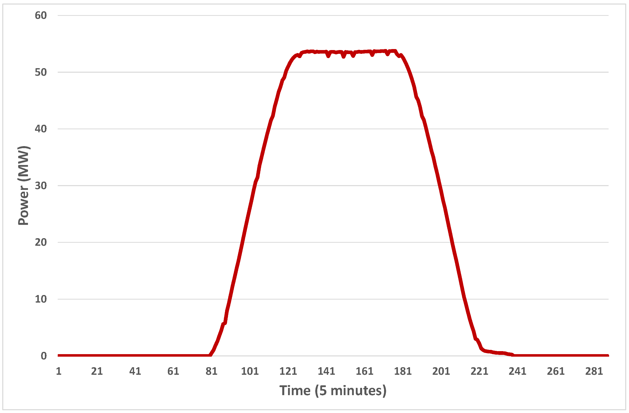
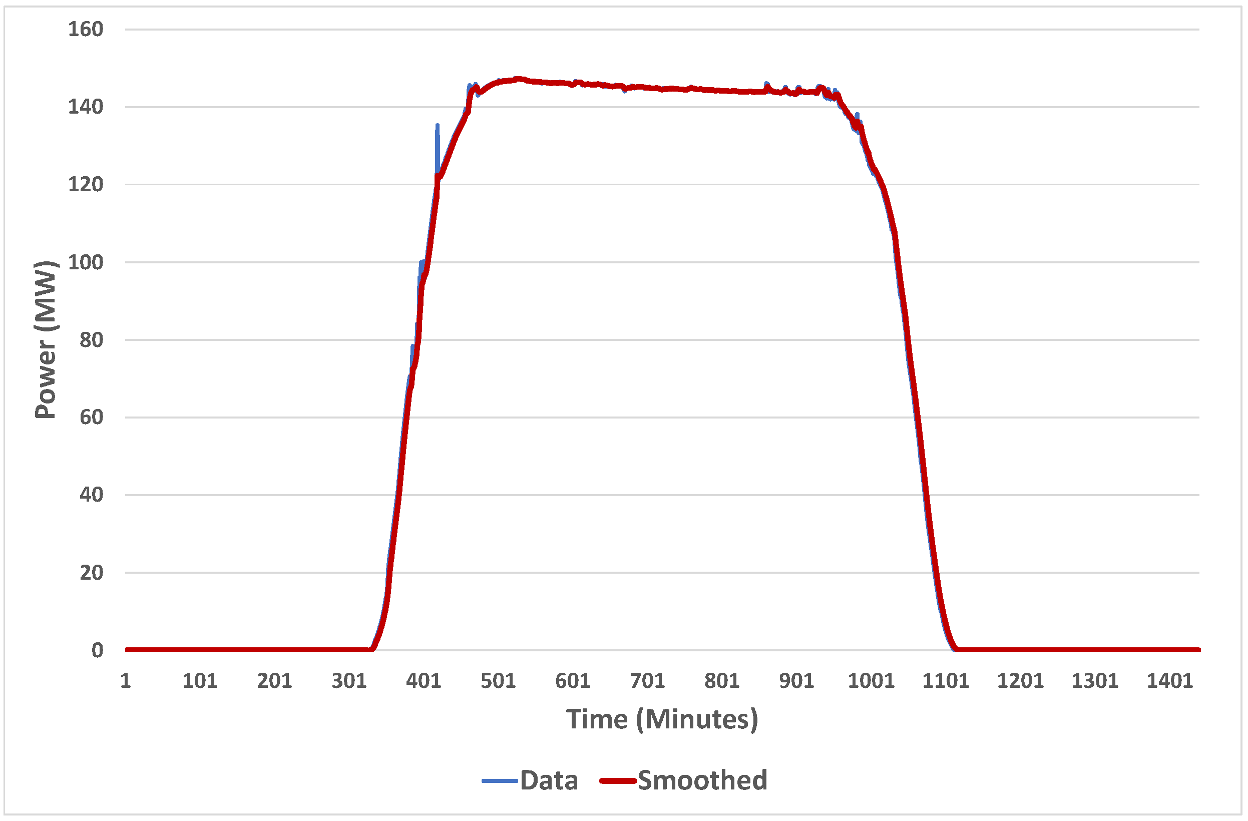
7.1. Characteristics of Power Output

There is at least one reason for our preference for dealing directly with wind farm output, rather than relying on wind speed and then using a power conversion model. That is the idea of where exactly on a wind farm do you measure the wind speed to obtain a representative idea of the wind resource for the whole farm.

For solar farms in Australia, there is a feature that must be taken into account. In most situations, there is an oversizing of the field of panels, as compared to the capacity of the inverters. This is performed, we suppose, to make the output nearly constant for a number of hours on a clear day—see Figure 1 for a clear day at the Broken Hill solar farm, in western New South Wales.

Note that the figure shows the profile for a clear day in summer. In winter on a clear day, the output will still reach the peak, but the time at the peak will be shorter on average, due to the sun being lower in the sky. So, as with clear sky model estimation for irradiance, we have to cater for seasonal variation if we are to define an empirical clear sky output (CSO) model for solar farms. Thus, the method we choose is to calculate the maximum value of the output for each time step of the day for the last thirty days. Then, we smooth these values using exponential smoothing. It could also be performed using a moving average. An illustration of this method is shown in Figure 2.

This structure is a parallel method to that of using a clear sky model (CSM) for irradiation (as in [16]), and converting GHI to a clear sky index (CSI) by dividing by the CSM. This CSI is used for forecasting, and then there is an inverse conversion to get back to GHI. If one wanted to do use GHI and thus CSI to forecast for a solar farm, it would then be necessary to have a power conversion model to get to the solar farm output. This would have to take into account the capping effect of the oversizing of the field that has been explained here. It would also have to take into account the changing features of the capping over the year. We suggest that for a solar farm, if one wants to use a clear sky index type of approach for forecasting, it would be better to use the output directly. One could divide the output at time t by the CSO at the same time to obtain a clear sky output index (CSOI). This would then be used for forecasting before back transforming to the output.

7.2. Value of Forecasts

We demonstrate in this section that due to goals specific to financial or societal outcomes, the models with superior forecasting skill do not necessarily display the greatest value. Antonanzas et al. [59] provide insight into this topic in evaluating the worth of day ahead forecasts for photovoltaics in the Spanish electricity market. They found in their study that the model with the highest quality produced also the best value; however, many of the other high performing models in terms of quality, that is low root mean square error (RMSE) or mean absolute error (MAE), did not perform as well in terms of value as models with lower quality. One other paper that makes a contribution to this topic is that of Yang et al. [16], but it only covers deterministic or point forecasts and is primarily focused on the verification of forecasts, rather than the value. There is a section in the paper dealing with value and we will expand on the topic here. One of the articles mentioned was that of Murphy [60], where he discusses what is a good forecast. He articulates three versions of goodness of forecasts. One is the correspondence between forecasters’ judgements and their forecasts. The next is the correspondence between the forecasts and the observations—the usual method of defining quality. Common measures of quality are detailed in Appendix A. The third is the benefits to the end user decision makers of the forecasts—the value. Matching the forecasts to the observations does not necessarily equate to increasing the value.

For example, in the SPEF forecasting trial [61], there was an interesting set of results of this mismatch. In

Table 3. Overall forecasting performance compared to ASEFS.

Site	Best Model (RMSE)	Skill	Best Model (MAE)	Skill
Darling Downs	Ensemble ML	9.2%	Ensemble Median	13.0%
Daydream	Ensemble Mean	16.2%	Ensemble Median	18.2%
Gannawarra	SkyCam	19.3%	Smart Persistence	16.8%
Emerald	Ensemble Mean	2.8%	ASEFS	-
Manildra	SkyCam	21.2%	SkyCam	16.6%

, where the best performing models are listed for the five solar farms, we can see that in each case they are either blended models, or the model using a sky camera and forecasting cloud movements from the images. However, when looking at which models saved the most in terms of lowering the Causer Pays fees (for taking the grid out of the required frequency limits),

Table 4. Financial performance compared to ASEFS, Australian Dollars.

Site	ASEFS Fee	Dispatch Model	Fee	Savings	Percentage Savings
Darling Downs	432,500	SF12	281,018	151,482	18%
Daydream	70,793	SF10	57,983	12,810	35%
Gannawarra	39,778	SF5	28,485	11,293	28%
Emerald	50,726	SF10	2129	48,595	98%
		Average	Savings	56,045	44%

, in each case, much more simple models, which did not perform very well in terms of RMSE and MAE compared to the blended models, actually had the highest monetary value to the farms. In fact, model $S{F}_{10}$, which performed best in terms of value at two of the farms, was the simplest model, combining Fourier series for the seasonality and an ARMA model for the stochastic component. It was simple enough to be re-estimated every five minutes, which may have helped in the monetary evaluation. Its overall skill in forecasting was not as good as the blended models, but its value was high.

In a situation where the system is photovoltaics plus storage and the operator is interacting with the NEM spot market in Australia, David et al. [62] found that there was an almost one to one correspondence between an improvement in MAE and an improvement in financial benefit. This was for day ahead forecasting of a solar farm with a simulated storage system added on. It may be that the addition of storage aided the correspondence, or perhaps it was because of working in the wholesale market, or a combination.

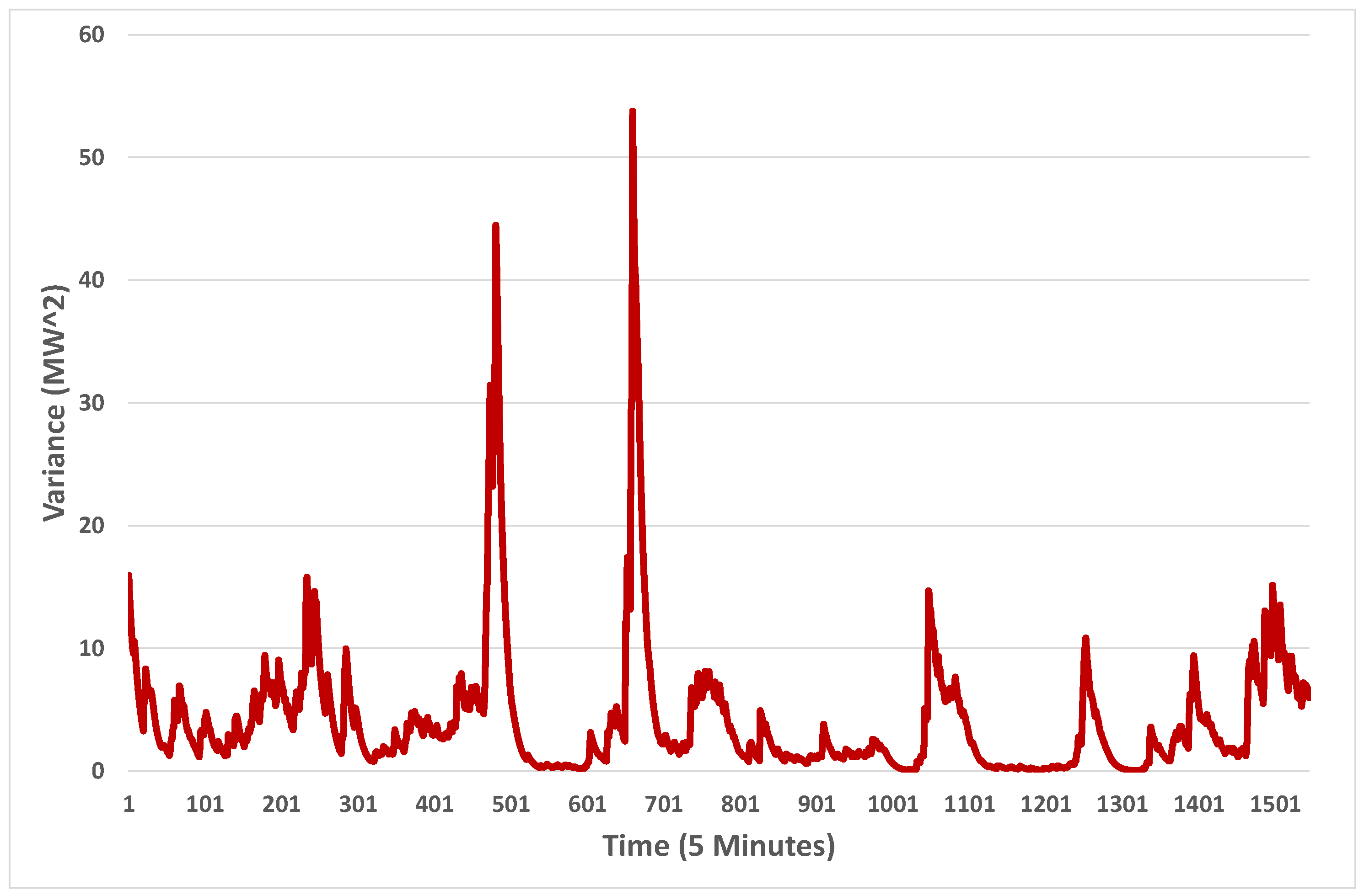
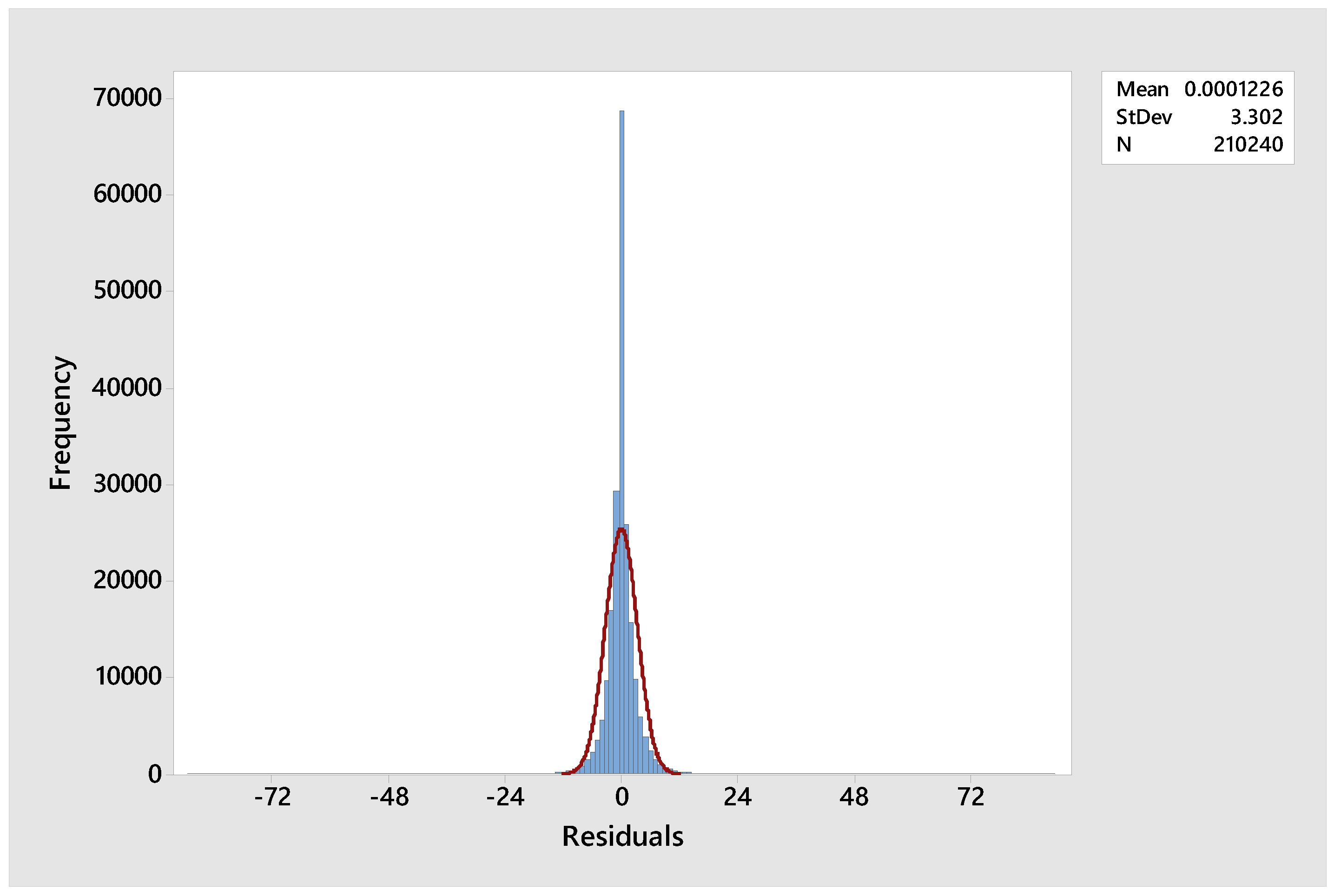
7.3. Heterogeneity of Variance

We suggest another area that has not had enough attention is the change of variance over time and its autocorrelative nature. As explained in [3,17,19], one has to cater for the change in variance in wind and solar, both resource and farm output, when performing probabilistic forecasting. An illustration of this effect is given in Figure 3, where we demonstrate how the variance over time using the exponentially weighted moving variance (EWMV) [63]. This is defined in the following way. First define the exponentially weighted moving average (EWMA).

$${\mu }_n=\lambda {\mu }_{n-1}+(1-\lambda )x_n$$

(5)

Then, the EWMV, $S_n$ is defined by

$$S_n=\alpha S_{n-1}+(1-\alpha )(x_n-{\mu }_n)(x_n-{\mu }_{n-1}).$$

(6)

In these determinations, $\lambda ,\alpha$ are in $(0, 1)$. It is obvious from the figure that an assumption of homogeneity of variance would be untenable. Further, if one examines the histogram of the noise terms after an autoregressive model is fitted to the output—see Figure 4—one can see that they do not follow a normal distribution and are an example of a fat tailed or leptokurtic distribution. So, in other words, the expectation that the noise will be white—independent and identically distributed—and also normally distributed, can not be justified. So, innovative means have to be employed to construct prediction intervals around a point forecast. In [3], the noise terms are transformed to the standard normal distribution, and then a model for the changing variance was constructed. From that error bounds were determined using the forecasted standard deviation and the scores from the standard normal distribution—see Equation (7) for a $95\%$ prediction interval. $B_{U,L}$ are the upper and lower bounds, and s is the forecasted standard deviation. These bounds are then back transformed and added to the point forecast.

$$B_{U,L}=\pm 1.96s$$

(7)

For solar farms, the construction of prediction intervals is even more involved, with the change in variance not only being conditional, as with wind farms, but also systematic, as the error distributions change with time of day and possibly time of year. How to deal with the systematic change of variance is demonstrated for solar irradiation in [17] and solar farms in [3]. Dealing with both the systematic and conditional change in variance is demonstrated for solar irradiation in [19]. Future work will apply this methodology for solar farms.

There is at least one other approach for interval forecasting for solar irradiation—the use of quantile regression. A very good description of the process for solar irradiation if given in [64]. We give a simple explanation of how this process works. One estimates the quantiles of the cumulative distribution of the variable of interest using a linear relationship between the variable y and explanatory variables x by

$$y=\beta x+ϵ$$

(8)

where $ϵ$ is a noise term.

Quantiles are estimated with assymetric weights applied to the mean absolute error (MAE). The quantile loss function is

$${\rho }_{\tau }=\left\{\begin{array}{cc}\tau u,\hfill & if u\ge 0\hfill \\ (\tau -1)u,\hfill & if u<0\hfill \end{array}\right.$$

(9)

where $\tau$ is the desired probability level.

The optimised quantity $\widehat{y}=\widehat{{\beta }_{\tau }}x$ is the result of finding the optimal $\beta$ using

$${\widehat{\beta }}_{\tau }=\underset{\beta }{min}\sum _{i=1}^n{\rho }_{\tau }(y_i-\beta x_i)$$

(10)

This optimisation can be performed for any $\tau$, and this can be used for any desired prediction interval estimation. We have performed this activity for some specific examples in a preliminary analysis and compared the results to those resulting from the approach of using the systematic change of variance in [3]. It appeared that the quantile regression approach is superior on specific types of days and the systematic version on others. Future work will attempt to use machine learning techniques to blend the two approaches to enhance the skill.

8. Conclusions

In this article we have put forward various methods to forecast wind speed and solar irradiation, added to a small number of papers that focus on forecasting output from installations as well. Additionally, we examined some papers that deal with an emerging topic in the area, that of forecasting of ramping events in solar farms. There is also a section on synthetic generation of solar irradiation series. The methods examined there can also be applied to similar problems with wind farms. However, as we have demonstrated, there are features of wind and solar farms that have not been substantially catered for in the literature. Thus, we have added sections with preliminary discussions on

• Clear sky output from solar farms, as compared to clear sky models for solar irradiation.
• Heterogeneity of solar and wind farm output.
• The value of forecasting, as compared to the skill of forecasting.

In future work we will concentrate on the three items listed here plus methods of blending of forecasts from different approaches, a feature that was shown to have higher skill than the individual tools in the SPEF project.

References

1. Diagne, M.; David, M.; Lauret, P.; Boland, J.; Schmutz, N. Review of solar irradiance forecasting methods and a proposition for small-scale insular grids. Renew. Sustain. Energy Rev. 2013, 27, 65–76. [Google Scholar] [CrossRef] [Green Version]
2. Farah, S.; Boland, J. Time series model for real-time forecasting of Australian photovoltaic solar farms power output. J. Renew. Sustain. Energy 2021, 13, 046102. [Google Scholar] [CrossRef]
3. Boland, J.; Farah, S. Probabilistic forecasting of wind and solar farm output. Energies 2021, 14, 5154. [Google Scholar] [CrossRef]
4. De Giorgi, M.G.; Congedo, P.M.; Malvoni, M. Photovoltaic power forecasting using statistical methods: Impact of weather data. IET Sci. Meas. Technol. 2014, 8, 90–97. [Google Scholar] [CrossRef]
5. Reikard, G. Predicting solar radiation at high resolutions: A comparison of time series forecasts. Sol. Energy 2009, 83, 342–349. [Google Scholar] [CrossRef]
6. Durrani, S.P.; Balluff, S.; Wurzer, L.; Krauter, S. Photovoltaic yield prediction using an irradiance forecast model based on multiple neural networks. J. Mod. Power Syst. Clean Energy 2018, 6, 255–267. [Google Scholar] [CrossRef]
7. De Giorgi, M.G.; Congedo, P.M.; Malvoni, M.; Laforgia, D. Error analysis of hybrid photovoltaic power forecasting models: A case study of mediterranean climate. Energy Convers. Manag. 2015, 100, 117–130. [Google Scholar] [CrossRef]
8. Rana, M.; Koprinska, I.; Agelidis, V.G. Univariate and multivariate methods for very short-term solar photovoltaic power forecasting. Energy Convers. Manag. 2016, 121, 380–390. [Google Scholar] [CrossRef]
9. Nespoli, A.; Ogliari, E.; Leva, S.; Massi Pavan, A.; Mellit, A.; Lughi, V.; Dolara, A. Day-Ahead Photovoltaic Forecasting: A Comparison of the Most Effective Techniques. Energies 2019, 12, 1621. [Google Scholar] [CrossRef] [Green Version]
10. Huang, J.; Korolkiewicz, M.; Agrawal, M.; Boland, J. Forecasting solar radiation on an hourly time scale using a Coupled AutoRegressive and Dynamical System (CARDS) model. Sol. Energy 2013, 87, 136–149. [Google Scholar] [CrossRef]
11. Huang, J.; Boland, J. Performance Analysis for One-Step-Ahead Forecasting of Hybrid Solar and Wind Energy on Short Time Scales. Energies 2018, 11, 1119. [Google Scholar] [CrossRef] [Green Version]
12. Colak, I.; Yesilbudak, M.; Genc, N.; Bayindir, R. Multi-period Prediction of Solar Radiation Using ARMA and ARIMA Models. In Proceedings of the 2015 IEEE 14th International Conference on Machine Learning and Applications (ICMLA), Miami, FL, USA, 9–11 December 2015; pp. 1045–1049. [Google Scholar] [CrossRef]
13. Boland, J.; David, M.; Lauret, P. Short term solar radiation forecasting: Island versus continental sites. Energy 2016, 113, 186–192. [Google Scholar] [CrossRef]
14. Fernandez-Jimenez, L.A.; Muñoz-Jimenez, A.; Falces, A.; Mendoza-Villena, M.; Garcia-Garrido, E.; Lara-Santillan, P.M.; Zorzano-Alba, E.; Zorzano-Santamaria, P.J. Short-term power forecasting system for photovoltaic plants. Renew. Energy 2012, 44, 311–317. [Google Scholar] [CrossRef]
15. Chu, Y.; Urquhart, B.; Gohari, S.M.I.; Pedro, H.T.C.; Kleissl, J.; Coimbra, C.F.M. Short-term reforecasting of power output from a 48 MWe solar PV plant. Sol. Energy 2015, 112, 68–77. [Google Scholar] [CrossRef]
16. Yang, D.; Alessandrini, S.; Antonanzas, J.; Antonanzas-Torres, F.; Badescu, V.; Beyer, H.G.; Blaga, R.; Boland, J.; Bright, J.M.; Coimbra, C.F.; et al. Verification of deterministic solar forecasts. Sol. Energy 2020, 210, 20–37. [Google Scholar] [CrossRef]
17. Grantham, A.; Gel, Y.; Boland, J. Nonparametric short-term probabilistic forecasting for solar radiation. Sol. Energy 2016, 133, 465–475. [Google Scholar] [CrossRef]
18. Ni, Q.; Zhuang, S.; Sheng, H.; Kang, G.; Xiao, J. An ensemble prediction intervals approach for short-term PV power forecasting. Sol. Energy 2017, 155, 1072–1083. [Google Scholar] [CrossRef]
19. Boland, J.; Grantham, A. Nonparametric Conditional Heteroscedastic Hourly Probabilistic Forecasting of Solar Radiation. J 2018, 1, 174–191. [Google Scholar] [CrossRef] [Green Version]
20. Golestaneh, F.; Pinson, P.; Gooi, H.B. Very short-term nonparametric probabilistic forecasting of renewable energy generation—With application to solar energy. IEEE Trans. Power Syst. 2016, 31, 3850–3863. [Google Scholar] [CrossRef] [Green Version]
21. Yagli, G.M.; Yang, D.; Srinivasan, D. Ensemble solar forecasting using data-driven models with probabilistic post-processing through GAMLSS. Sol. Energy 2020, 208, 612–622. [Google Scholar] [CrossRef]
22. David, M.; Ramahatana, F.; Trombe, P.J.; Lauret, P. Probabilistic forecasting of the solar irradiance with recursive ARMA and GARCH models. Sol. Energy 2016, 133, 55–72. [Google Scholar] [CrossRef] [Green Version]
23. Ahmed, R.; Sreeram, V.; Mishra, Y.; Arif, M.D. A review and evaluation of the state-of-the-art in PV solar power forecasting: Techniques and optimization. Renew. Sustain. Energy Rev. 2020, 124, 109792. [Google Scholar] [CrossRef]
24. Zhang, Y.; Wang, J.; Wang, X. Review on probabilistic forecasting of wind power generation. Renew. Sustain. Energy Rev. 2014, 32, 255–270. [Google Scholar] [CrossRef]
25. Sun, M.; Feng, C.; Chartan, E.K.; Hodge, B.M.; Zhang, J. A two-step short-term probabilistic wind forecasting methodology based on predictive distribution optimization. Appl. Energy 2019, 238, 1497–1505. [Google Scholar] [CrossRef]
26. Jin, H.; Shi, L.; Chen, X.; Qian, B.; Yang, B.; Jin, H. Probabilistic wind power forecasting using selective ensemble of finite mixture Gaussian process regression models. Renew. Energy 2021, 174, 1–18. [Google Scholar] [CrossRef]
27. Kim, Y.; Hur, J. An ensemble forecasting model of wind power outputs based on improved statistical approaches. Energies 2020, 13, 1071. [Google Scholar] [CrossRef] [Green Version]
28. Jiang, Y.; Zheng, L.; Ding, X. Ultra-short-term prediction of photovoltaic output based on an LSTM-ARMA combined model driven by EEMD. J. Renew. Sustain. Energy 2021, 13, 1–14. [Google Scholar] [CrossRef]
29. Mellit, A.; Pavan, A.M.; Ogliari, E.; Leva, S.; Lughi, V. Advanced methods for photovoltaic output power forecasting: A review. Appl. Sci. 2020, 10, 487. [Google Scholar] [CrossRef] [Green Version]
30. Chen, B.; Lin, P.; Lai, Y.; Cheng, S.; Chen, Z.; Wu, L. Very-Short-Term Power Prediction for PV Power Plants Using a Simple and Effective RCC-LSTM Model Based on Short Term Multivariate Historical Datasets. Electronics 2020, 9, 289. [Google Scholar] [CrossRef] [Green Version]
31. AlKandari, M.; Ahmad, I. Solar power generation forecasting using ensemble approach based on deep learning and statistical methods. Appl. Comput. Inform. 2020; ahead-of-print. [Google Scholar] [CrossRef]
32. Delgado, I.; Fahim, M. Wind Turbine Data Analysis and LSTM-Based Prediction in SCADA System. Energies 2020, 14, 125. [Google Scholar] [CrossRef]
33. Ibrahim, M.; Alsheikh, A.; Al-Hindawi, Q.; Al-Dahidi, S.; ElMoaqet, H. Short-Time Wind Speed Forecast Using Artificial Learning-Based Algorithms. Comput. Intell. Neurosci. 2020, 2020, 1–15. [Google Scholar] [CrossRef]
34. Wang, H.; Yi, H.; Peng, J.; Wang, G.; Liu, Y.; Jiang, H.; Liu, W. Deterministic and probabilistic forecasting of photovoltaic power based on deep convolutional neural network. Energy Convers. Manag. 2017, 153, 409–422. [Google Scholar] [CrossRef]
35. Alessandrini, S.; Delle Monache, L.; Sperati, S.; Cervone, G. An analog ensemble for short-term probabilistic solar power forecast. Appl. Energy 2015, 157, 95–110. [Google Scholar] [CrossRef] [Green Version]
36. van der Meer, D.W.; Shepero, M.; Svensson, A.; Widén, J.; Munkhammar, J. Probabilistic forecasting of electricity consumption, photovoltaic power generation and net demand of an individual building using Gaussian Processes. Appl. Energy 2018, 213, 195–207. [Google Scholar] [CrossRef]
37. Pinson, P. Very-short-term probabilistic forecasting of wind power with generalized logit-normal distributions. J. R. Stat. Soc. Ser. Appl. Stat. 2012, 61, 555–576. [Google Scholar] [CrossRef]
38. Tahmasebifar, R.; Moghaddam, M.P.; Sheikh-El-Eslami, M.K.; Kheirollahi, R. A new hybrid model for point and probabilistic forecasting of wind power. Energy 2020, 211, 119016. [Google Scholar] [CrossRef]
39. Taylor, J.W. Probabilistic forecasting of wind power ramp events using autoregressive logit models. Eur. J. Oper. Res. 2017, 259, 703–712. [Google Scholar] [CrossRef]
40. Abuella, M.; Chowdhury, B. Forecasting of solar power ramp events: A post-processing approach. Renew. Energy 2019, 133, 1380–1392. [Google Scholar] [CrossRef]
41. Probst, O.; Minchala, L.I. Mitigation of short-term wind power ramps through forecast-based curtailment. Appl. Sci. 2021, 11, 4371. [Google Scholar] [CrossRef]
42. Han, L.; Qiao, Y.; Li, M.; Shi, L. Wind power ramp event forecasting based on feature extraction and deep learning. Energies 2020, 13, 6449. [Google Scholar] [CrossRef]
43. Australian Energy Market Operator. Renewable Integration Study Appendix C: Managing variability and uncertainty. 2020, pp. 1–77. Available online: https://aemo.com.au/en/energy-systems/major-publications/renewable-integration-study-ris (accessed on 11 June 2021).
44. Brinkworth, B. Autocorrelation and stochastic modelling of insolation sequences. Sol. Energy 1977, 19, 343–347. [Google Scholar] [CrossRef]
45. Balouktsis, A.; Tsalides, P. Stochastic simulation model of hourly total solar radiation. Sol. Energy 1986, 37, 119–126. [Google Scholar] [CrossRef]
46. Phillips, W. Harmonic analysis of climatic data. Sol. Energy 1984, 32, 319–328. [Google Scholar] [CrossRef]
47. Boland, J. Time-series analysis of climatic variables. Sol. Energy 1995, 55, 377–388. [Google Scholar] [CrossRef]
48. Sfeir, A. A stochastic model for predicting solar system performance. Sol. Energy 1980, 25, 149–154. [Google Scholar] [CrossRef]
49. Aguiar, R.; Collares-Pereira, M.; Conde, J. Simple procedure for generating sequences of daily radiation values using a library of Markov transition matrices. Sol. Energy 1988, 40, 269–279. [Google Scholar] [CrossRef]
50. Aguiar, R.; Collares-Pereira, M. Statistical properties of hourly global radiation. Sol. Energy 1992, 48, 157–167. [Google Scholar] [CrossRef]
51. Aguiar, R.; Collares-Pereira, M. TAG: A time-dependent, autoregressive, Gaussian model for generating synthetic hourly radiation. Sol. Energy 1992, 49, 167–174. [Google Scholar] [CrossRef]
52. Amato, U.; Andretta, A.; Bartoli, B.; Coluzzi, B.; Cuomo, V.; Fontana, F.; Serio, C. Markov processes and Fourier analysis as a tool to describe and simulate daily solar irradiance. Sol. Energy 1986, 37, 179–194. [Google Scholar] [CrossRef]
53. Graham, V.; Hollands, K. A method to generate synthetic hourly solar radiation globally. Sol. Energy 1990, 44, 333–341. [Google Scholar] [CrossRef]
54. Bright, J.M. Synthetic Solar Irradiance Modeling Solar Data; AIP Publishing LLC: Melville, NY, USA, 2021. [Google Scholar]
55. Boland, J.; Grantham, A. Principles and Key Applications: Principles and Applications of Synthetic Solar Irradiance; AIP Publishing LLC: Melville, NY, USA, 2021; pp. 2-1–2-32. [Google Scholar] [CrossRef]
56. Grantham, A.; Pudney, P.; Ward, L.; Belusko, M.; Boland, J. Generating synthetic five-minute solar irradiance values from hourly observations. Sol. Energy 2017, 147, 209–221. [Google Scholar] [CrossRef]
57. Grantham, A.; Pudney, P.; Boland, J. Generating synthetic sequences of global horizontal irradiation. Sol. Energy 2018, 162, 500–509. [Google Scholar] [CrossRef]
58. Larrañeta, M.; Fernandez-Peruchena, C.; Silva-Pérez, M.A.; Lillo-bravo, I.; Grantham, A.; Boland, J. Generation of synthetic solar datasets for risk analysis. Sol. Energy 2019, 187, 212–225. [Google Scholar] [CrossRef]
59. Antonanzas, J.; Pozo-Vázquez, D.; Fernandez-Jimenez, L.A.; Martinez-de Pison, F.J. The value of day-ahead forecasting for photovoltaics in the Spanish electricity market. Sol. Energy 2017, 158, 140–146. [Google Scholar] [CrossRef]
60. Murphy, A.H. What is a good forecast? An essay on the nature of goodness in weather forecasting. Weather Forecast. 1993, 8, 281–293. [Google Scholar] [CrossRef] [Green Version]
61. Snell, T.; Consani, S.; West, S.; Amos, M. Solar Power Ensemble Forecaster Final Report—Public; Industrial Monitoring and Control: Newcastle, Australia, 2021. [Google Scholar]
62. David, M.; Boland, J.; Cirocco, L.; Lauret, P.; Voyant, C. Value of deterministic day-ahead forecasts of PV generation in PV + Storage operation for the Australian electricity market. Sol. Energy 2021, 224, 672–684. [Google Scholar] [CrossRef]
63. Finch, T. Incremental Calculation of Weighted Mean and Variance; University of Cambridge: Cambridge, UK, 2009; Volume 1, pp. 1–8. [Google Scholar]
64. Lauret, P.; David, M.; Pedro, H.T. Probabilistic solar forecasting using quantile regression models. Energies 2017, 10, 1591. [Google Scholar] [CrossRef]
Figure 1. Clear day output in Broken Hill. Time is in 5 min intervals, with 288 intervals per day.
Energies 15 00370 g001
Figure 2. Clear day output in Broken Hill.
Energies 15 00370 g002
Figure 3. Exponentially weighted moving variance. Time is in 5 min intervals.
Energies 15 00370 g003
Figure 4. Histogram of wind farm output noise with normal curve overlaid.
Energies 15 00370 g004