Article

A Neural Network-Inspired Matrix Formulation of Chemical Kinetics for Acceleration on GPUs

Department of Aerospace Engineering, University of Michigan, Ann Arbor, MI 48109, USA
*
Author to whom correspondence should be addressed.
Energies 2021, 14(9), 2710; https://doi.org/10.3390/en14092710
Submission received: 21 March 2021 / Revised: 1 May 2021 / Accepted: 4 May 2021 / Published: 9 May 2021

Abstract

:
High-fidelity simulations of turbulent flames are computationally expensive when using detailed chemical kinetics. For practical fuels and flow configurations, chemical kinetics can account for the vast majority of the computational time due to the highly non-linear nature of multi-step chemistry mechanisms and the inherent stiffness of combustion chemistry. While reducing this cost has been a key focus area in combustion modeling, the recent growth in graphics processing units (GPUs) that offer very fast arithmetic processing, combined with the development of highly optimized libraries for artificial neural networks used in machine learning, provides a unique pathway for acceleration. The goal of this paper is to recast Arrhenius kinetics as a neural network using matrix-based formulations. Unlike ANNs that rely on data, this formulation does not require training and exactly represents the chemistry mechanism. More specifically, connections between the exact matrix equations for kinetics and traditional artificial neural network layers are used to enable the usage of GPU-optimized linear algebra libraries without the need for modeling. Regarding GPU performance, speedup and saturation behaviors are assessed for several chemical mechanisms of varying complexity. The performance analysis is based on trends for absolute compute times and throughput for the various arithmetic operations encountered during the source term computation. The goals are ultimately to provide insights into how the source term calculations scale with the reaction mechanism complexity, which types of reactions benefit the GPU formulations most, and how to exploit the matrix-based formulations to provide optimal speedup for large mechanisms by using sparsity properties. Overall, the GPU performance for the species source term evaluations reveals many informative trends with regards to the effect of cell number on device saturation and speedup. Most importantly, it is shown that the matrix-based method enables highly efficient GPU performance across the board, achieving near-peak performance in saturated regimes.

1. Introduction

Computational modeling of reacting flows has become an integral part of the design and analysis of complex propulsion concepts [1,2]. While a wide variety of tools constitute the modeling pathways, simulations for reacting flows require detailed models for chemical reactions. In most applications, the multi-physics behavior stemming from chemical reactions induces a highly complex Arrhenius-based expression for the species source terms, the nonlinearity of which produces an extremely stiff set of equations for the time evolution of the reacting chemical species [1,2,3]. The wide range of timescales in this setting must be resolved to accurately represent the characteristic turbulence–chemistry interactions.
As a result, efforts to accelerate the computation of turbulent reacting flows with a focus on the chemical reaction (kinetics) terms have been, and still is, a major research effort in fields related to turbulent combustion. The efforts can be categorized into two classes: The first, more traditional class is model-oriented, i.e., an approximation to the exact formulation for the source terms and the species evolution is constructed with the goal of decreasing the time-to-solution. The second class, which is the central focus of this work, is hardware-oriented, i.e., the computation of the source terms and time-evolution of the species is accelerated by porting existing exact algorithms to state-of-the-art hardware. The former is driven by innovations in physical understanding, whereas the latter is driven by advances in emerging heterogeneous computing architecture. To motivate the need for the latter, some previous work concerning the former class (traditional modeling approaches) is first briefly reviewed. Note that both classes are not mutually exclusive—the tools presented by machine learning (namely neural networks), to be touched on further below, very much blur the line between the two.
While there has been considerable growth in the physical understanding and the development of reliable yet computationally efficient models [1,2], representation of complex chemical kinetics remains a challenge. In particular, the use of detailed mechanisms that involve a hundred or more species and an even larger number of reactions in a turbulent flow configuration remains out of reach [4]. Although progress towards their use in canonical flows has been reported [5], their use in the simulation of complex geometries is still limited. When modeling turbulent combustion, manifold methods have overcome this computational issue by representing multi-step kinetics using a reduced-set of tracking variables such as mixture fraction and progress variable [6]. However, other combustion models such as the transported probability density function (PDF) approach [7,8] or the linear-eddy model [9] require detailed chemistry to be directly evolved. In this regard, methods and algorithms that allow detailed chemical processes to be included in such approaches are a critical requirement.
Models that attempt to tackle this issue from a reduction point of view include tabulation methods such as in-situ adaptive tabulation (ISAT) [10] and the PRISM [11] approach. In these methods, the computationally expensive numerical integration of chemical source terms, which can be cast as a set of ordinary differential equations (ODEs), is replaced by a look-up table. In particular, ISAT builds a trust region in thermochemical composition space using a set of ellipsoids determined by the Jacobian of the source terms. The cost of building and accessing such tables, however, can become expensive for large mechanisms, especially on modern high-performance computers (HPCs) that are memory-limited and use extensive concurrency in computations to reach high throughput efficiency. For these reasons, alternative data-driven modeling approaches based on artificial neural networks (ANNs) [12,13,14,15,16] have become increasingly popular, although they introduce additional issues related to model robustness and training data quality (the dependence on data is, in general, a disadvantage in applications for which both the physical constraints are already well understood and the mechanism sizes are large).
Despite this, the critical enabling tool for ANNs is the development of hardware for machine learning (ML) in light of modern exascale computing goals [17]. To conform to the societal demands of the ML technology, modern state-of-the-art HPCs have moved almost all compute power into graphics processing units (GPUs) or similar many-core accelerators, whose hardware architectures enable fast algorithm execution in single-instruction, multiple-thread (SIMT) environments [18]. Alongside providing much higher theoretical peak performances, the shift in HPC compute power towards GPUs is also advantageous due to their increased power efficiency. It has therefore become crucial for the CFD community to adapt to these changes, though a central issue revolves around the re-interpretation and re-design of traditional algorithms that have been around for decades into a GPU-optimal scope [19].
In general, GPUs operate differently from CPUs, requiring the algorithmic implementations for expensive routines, such as the aforementioned source term computations, to be altered in order to leverage their specific hardware architecture to extract as much computational gain as possible. To this end, approaches for GPU-offloading for chemical kinetics have been explored in detail in recent years to success [20,21,22], and their implementation into high-fidelity parallel solvers has also been demonstrated [23]. These approaches traditionally rely on translation of the exact equations for kinetics and time-integration methods into the GPU environment. However, much of the literature in the context of kinetics offloading has been geared towards either the time-integration aspect of the kinetics problem [19,22] or the role of the kinetics offloading in the context of a full reacting flow solver [23], and not on the computationally intensive evaluation of the source terms in isolation.
As such, the underlying goal of this work is to provide a GPU offloading strategy for an alternative, matrix-based viewpoint of the offloading problem for the chemical source term computation alone. The methodology is designed to supplement other related GPU-optimal techniques, such as stiff time-integration methods, that rely on the source term evaluation explicitly. One major thrust is to show how the exact formulations for the species source terms can be interpreted as neural network layers without the need for any models, thus facilitating a GPU-optimal matrix-oriented methodology that is both accurate and well suited for emerging HPC architectures. Another thrust is to assess how the complexity of the individual reaction mechanisms themselves affects the GPU performance. By means of a detailed cost and throughput breakdown, the central idea is to illuminate the fact that certain types of reactions, the set of which constitute a portion of a chemical mechanism used to parameterize the source term evaluation, are more suitable for GPU offloading than others. Further, it is shown how the underlying matrix multiplication algorithms can be modified to enhance GPU performance for very large mechanisms through the use of sparsity properties that arise from physical constraints tied to the elementary building-block reactions. Alongside providing a methodology for an efficient GPU-based routine for chemical kinetics, a subsidiary goal is to hopefully provide information that enables the design of more GPU-optimal chemical mechanisms for usage in multi-physics CFD solvers from the get-go.
The remainder of the paper proceeds as follows. In Section 2, the methodology for the matrix-inspired formulation is presented in the language of artificial neural networks, and a classification of reaction types that facilitates the GPU performance analysis is provided. In Section 3, the GPU performance is assessed in detail from a compute time and throughput perspective, the costs of individual reaction types are assessed, and a pathway for improving the speedup for very large mechanisms is provided. Concluding remarks and future directions are given in Section 4.

2. Methodology

This section first summarizes the chemical kinetic equations from a matrix-based perspective (Section 2.1), and then discusses the data structure and organization of the matrices used in the GPU computations (Section 2.2). The matrix-based formulations are presented in the language of traditional artificial neural networks (ANNs) where appropriate. Conveying the exact formulation of the source term computation with ANNs is intended to inform the reader that the form of kinetics equations as-is is efficiently described via neural network layers without any need for training or modeling. For this reason, the authors believe the ANN connections can lead to valuable insights regarding the general interpretation and potential design of GPU-optimal chemical mechanisms. Additionally, the neural network connections open pathways for constrained modeling approaches, here called “approximate ANNs”, which can be designed to reduce the overall computational effort undertaken during the exact source term computation at the cost of perfect accuracy. Although it does not fall into the main scope of this work, additional details on the approximate ANN formulation are provided in Appendix A for the interested reader.
Of special importance in Section 2.2, and tied to the matrix data structures explained therein, is the distribution of different reaction types present in a given mechanism. In general, different algorithms are required for different reaction types—some allow for matrix formulations and others do not. As such, a characterization of chemical mechanisms based on the distribution of these reaction types is presented to provide a pathway for assessing: (a) how beneficial the matrix representation can be for a particular mechanism; and (b) how the prevalence of specific reaction types can positively or negatively impact the GPU-derived speedup. The main reason for introducing the reaction-type classification is to bring forward the idea that, in the determination of GPU speedup, mechanism species and reaction numbers are not the only factors; the complexity of the individual reactions themselves also plays an important role.

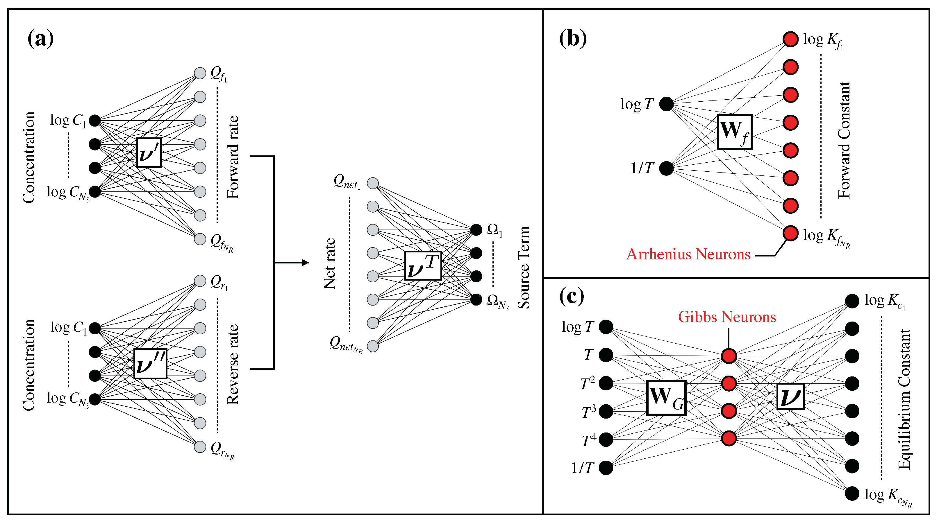
2.1. Matrix-Based Kinetics Equations

In the following, the quantities N C , N S , and N R denote the batch size (which can be interpreted as the number of reacting cells in a domain offloaded to the GPU), number of species, and number of reactions, respectively. Unless otherwise indicated, matrices are denoted by bold symbols (e.g., A ) and vectors by non-bold symbols (e.g., a). The scalar entry of matrix A in row i and column j is denoted A i j ; similarly, the scalar ith entry of vector a is denoted a i . Further, the quantities i, j, and k index N C , N R , and N S , respectively (i.e., i = 1 , , N C , j = 1 , , N R , and k = 1 , , N S ). For the set of species { S 1 , , S N S } , a general chemical mechanism is represented as
k = 1 N S ν k j S k k = 1 N S ν k j S k , j = 1 , , N R ,
where ν R N S × N R (respectively, ν ) is the reactant (respectively, product) stoichiometric coefficient matrix and ν = ν ν . The formulations below proceed, without loss of generality, in the context that all N R reactions are reversible. In practice, as discussed in greater detail in Section 2.3, this may not be the case.
The molar net production rate ( kmol / m 3 s ) for species k in cell i is
Ω i k = j = 1 N R ν k j Q n e t i j ,
where Ω R N C × N S contains the source terms and Q n e t R N C × N R contains the net reaction rates. Note that Equation (2) can be expressed concisely through the matrix multiplication Ω = Q n e t ν T . The complexity comes from the net reaction rate, which is expressed as
Q n e t i j = Q f i j Q r i j = K f i j k = 1 N S C i k ν k j K r i j k = 1 N S C i k ν k j .
Above, Q f and Q r R N C × N R are the forward and reverse reaction rate matrices, respectively; K f and K r R N C × N R are the forward and reverse rate constants, respectively; and C R N C × N S contains the species molar concentrations. Since Q f and Q r are non-negative, Equation (3) can be interpreted as a summation of two ANN layers by enabling matrix multiplications in the logarithm space:
Q n e t = exp log ( C ) ν + log ( K f ) exp log ( C ) ν + log ( K r ) .
It can be seen through Equation (4) that the forward and reverse contributions are ANN layers with exponential activation functions, where the input is the logarithm of the concentration matrix C , the weight matrices are known stoichiometric coefficients ν and ν , and the biases are the logarithms of rate constants K f and K r for the forward and reverse contributions, respectively. These rate constant bias terms can also be interpreted as neural network layers and are the subjects of discussion further below.
Figure 1a summarizes the above formulation (Equations (2) and (4)) through an ANN architecture. Note that the leading matrix dimension of all input and output variables, which constitutes the batch size in the forward pass, is N C . This allows for efficient threading and fast execution in high fidelity settings, assuming optimized linear algebra libraries (such as cuBLAS [24]) are utilized by the user. The remaining task, described below, is to obtain the rate constants K f and K r .
The forward rate constant K f R N C × N R is given by the Arrhenius expression
K f i j = A j T i β j exp E j R T i ,
where A, β , and E are vectors each of size N R containing pre-exponential factors, temperature exponents, and activation energies respectively for the elementary reactions. These Arrhenius parameters are known to the user through the mechanism files. The natural logarithm of the forward rate (required in Equation (4)) usefully yields a form that can also be interpreted as a linear ANN layer,
log ( K f ) = X f W f + B f , where
X f = log T 1 1 / T 1 log T 2 1 / T 2 log T N C 1 / T N C , W f = β 1 β N R E 1 / R E N R / R , B f = log A 1 log A 2 log A N R T .
In Equation (6), X f R N C × 2 is the temperature-dependent input, W f R 2 × N R is a weight matrix consisting of temperature exponents and activation energies, and B f R 1 × N R is a bias term of pre-exponential factors. In this sense, each row of the layer output log ( K f ) can be interpreted as a set of N R Arrhenius neurons.
The reverse rate constant K r R N C × N R is given by
K r i j = K f i j / K c i j ,
where K c R N C × N R contains the equilibrium rate constants. Since the expression for log ( K f ) is provided through the Arrhenius neurons (Equation (6)), the task of determining log ( K r ) required in Equation (4) is accomplished by considering only log ( K c ) .
The equilibrium constant for cell i and reaction j is [25]
K c i j = p r e f R T i k ν k j exp Δ S j ( T i ) R Δ H j ( T i ) R T i ,
where Δ S j and Δ H j are changes in entropy and enthalpy for reaction j, and p r e f is the reference pressure (1 bar). The logarithm of Equation (8) yields
log ( K c i j ) = k = 1 N S ν j k G i k + p r e f R T i ,
where G R N C × N S is the nondimensional Gibbs free energy matrix (hereafter referred to as the Gibbs matrix) obtained from the nondimensional enthalpy ( H R N C × N S ) and entropy ( S R N C × N S ) matrices. Each entry in the Gibbs matrix is determined from NASA polynomials which provide species enthalpy and entropy as tabulated functions of temperature. The result can be expressed as a matrix multiplication
G = H S = X G W G + B G , where
X G = log T 1 T 1 T 1 2 T 1 3 T 1 4 1 / T 1 log T 2 T 2 T 2 2 T 2 3 T 2 4 1 / T 2 log T N C T N C T N C 2 T N C 3 T N C 4 1 / T N C , W G = α 1 , 1 α 1 , N S α 2 , 1 α 2 , N S α 6 , 1 α 6 , N S , B G = α 7 , 1 α 7 , 2 α 7 , N S T .
In Equation (10), X G R N C × 6 is the input consisting of various functions of temperature and α R 7 × N S is a matrix of polynomial coefficients; the first six rows of α is the weight matrix W G and the last row is the bias B G . Note that, although not shown in Equation (10) for conciseness, the quantities in α (and in turn W G and B G ) are also functions of the cell temperature T i and the species index. This is because the species polynomial coefficients change based on a cutoff temperature (usually 1000 K). Regarding practical implementation, in the case that the NASA cutoff temperature is the same for all of the species (say 1000 K), it is possible to treat the evaluation of Equation (10) (the first layer in Figure 1c) with linear algebra libraries (i.e., cuBLAS operations) by populating two copies of α based on the cutoff threshold. However, this approach is only feasible in the case when the NASA cutoff temperature is the same for all of the species. In the more general case where the cutoff temperature varies with the species index, it is much more convenient to directly treat the evaluation of Equation (10) using a custom matrix multiplication kernel that computes the polynomial directly—with conditional logic that populates the values in α on-the-fly based on the cell temperature—instead of a using the cuBLAS (or other similar) routines. The convenience here outweighs the hit on GPU optimality, and, as such, this is the approach used in the GPU implementation profiled in Section 3. It should be noted that a principle advantage in considering the matrix form for the evaluation of NASA polynomials (as in Equation (10)) comes with the approximate ANN framework (see Appendix A)—the framework overcomes the conditional logic limitations imposed by the NASA coefficients by designing a neural network to essentially discover new polynomials such that the equilibrium rate constants can be recovered, but the coefficients’ dependence on temperature is removed.
Inserting Equation (10) into Equation (9) gives
log ( K c ) = ( X G W G + B G ) ν ,
where the standard concentration term p r e f / R T i has been integrated into the bias B G . Equation (11) can be interpreted as a linear two-layer ANN. The parameters of the first layer (the Gibbs layer) are the temperature-dependent W G and B G and those of the second layer are the net stoichiometric coefficients ν . The intermediary neurons (i.e., hidden layer neurons) here are referred to as the Gibbs neurons.
Illustrations of both the forward and the equilibrium rate constant formulations as neural network-inspired architectures are shown in Figure 1b,c, with Arrhenius and Gibbs neurons highlighted. Alongside the formulations provided above, however, some additional complications arise when considering the forward rate constant in detailed reaction mechanisms and the treatment of zero concentrations. These are considered in the present work and brief descriptions on their implementation are described below.
To handle three-body reactions, the quantity log ( M ) is added to log ( K f ) , where M R N C × N R is a matrix of third-body concentrations for each reaction ( M i j is 1 if reaction j does not include a third body). The entries in M can be obtained through the matrix multiplication M = C E , where E R N S × N R is a matrix of third-body efficiency factors. In practice, for computational savings, the third body concentration matrix equation is evaluated only for the subset of total reactions N R , since third body concentration terms are generally not present in every single reaction.
Additionally, falloff and pressure-log reactions, which constitute two of the reaction types discussed further below in Section 2.2, are treated separately from standard Arrhenius reactions as defined in Equation (6). In summary, they modify the standard matrix-based formulation of the forward rate constant logarithm by incorporating much more complex and arithmetically intensive expressions. As such, pressure-log and falloff formulations such as that of Lindemann, Troe, or SRI are handled on the GPU in a custom non-matrix fashion. More information on the mathematical implementation expressions for these reactions can be found in the Cantera and Chemkin documentation [26,27].
Lastly, it is necessary to acknowledge that the treatment of kinetics in the logarithm space introduces scenarios in which logarithms of zero concentration are required. There are several ways to treat this with effectively zero propagating error—some options are listed below.
  • Let the GPU handle the zero concentrations natively. For example, CUDA supports the operation of exp(log(0))=0 through the Inf floating point placeholder. That is, CUDA ensures that the operation log(0)=-Inf, and that exp(-Inf)=0.
  • Replace either the zero concentrations or mass fractions with an extremely small positive number and then proceed with the computations. This number should be small enough (i.e., 1.0e-300) to effectively produce a huge negative number upon taking the logarithm.
  • Replace the logarithm of the zero concentrations directly with a huge negative number, e.g., through a re-definition as log(0)=-1.0e300.
It should be noted that errors are indeed introduced from all of the above treatments of the zero logarithm, as it is mathematically undefined and the numerical treatments incur some truncation penalties. However, these errors are microscopic relative to other error sources that are encountered in a reacting flow simulation and are unnoticeable in practice. The reader is referred to Appendix B for additional verification, which provides sample results using the second option.

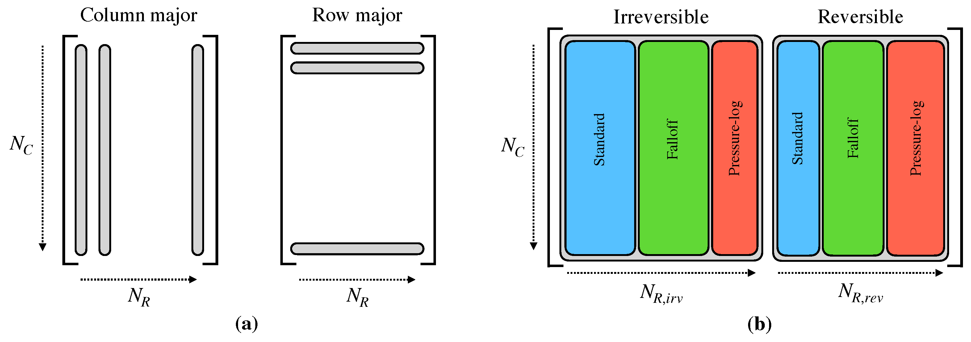
2.2. Organization of Data

The notion of N C , N R , and N S introduces three matrix types that represent the backbone of the methodology discussed above: an N C × N R reaction matrix, an N C × N S species matrix, and an N S × N R (or the transpose) stoichiometric matrix. As per the formulations in Section 2.1, reaction matrices are used to define quantities such as rate constants and reaction rates, whereas species matrices are used to define concentrations, mass fractions and species net production rates. Stoichiometric matrices can be interpreted as tools that transform a matrix from the species representation to the reaction representation or vice versa.
Assuming the matrices occupy contiguous blocks of memory, there are two ways to go about their storage: a row-major or a column-major representation. As an example, consider some given N C × N R matrix A (a reaction matrix). In the row-major format, the reaction matrix is represented as an N C -sized stack of 1 × N R row vectors. On the other hand, in the column-major format, the matrix is interpreted as an N R -sized stack of N C × 1 column vectors. This difference is shown in Figure 2a. There are a few reasons the column-major representation is more beneficial here. First, in most realistic high-fidelity applications, we have the condition N C N R > N S . From a GPU efficiency perspective, it is important to have memory coalescence along the highest dimension N C , which necessitates a column-major storage format for A . (Good coalescence ensures that, for a given number of floating point operations (FLOPs) in the kernel, the FLOPs executed by the GPU per byte of transferred global memory (arithmetic intensity) is as high as possible. Arithmetic intensity is used as a general metric to assess GPU performance, and it is discussed further in Section 3.1. For more information on the specifics of global memory coalescence, the reader is referred to the CUDA toolkit documentation.) Second, the practical implications of designing a matrix as a collection of N C × 1 vectors is appealing—it allows for naturally extracting contiguous N C × N X subsets of the A matrix, where N X N R . This becomes especially useful when dealing with different reaction types as discussed in Section 2.3. Lastly, the column-major format allows for seamless integration with cuBLAS, a highly efficient GPU-based linear algebra library.

2.3. Reaction Decomposition and Classification

As mentioned in Section 2.1, not all reactions need to be reversible in a given mechanism. Oftentimes, Arrhenius parameters for reverse rate constants are provided directly, in which case a physically reversible reaction is supplied to the user through the mechanism files as two irreversible (forward) reactions parameterized by the corresponding Arrhenius constants. In this scenario, the computation of the equilibrium rate constant (Equation (9)) for one reaction is effectively traded for an additional Arrhenius rate constant evaluation (Equation (6)).
With this in mind, any given reaction matrix A initialized as a contiguous column-major matrix of size N C × N R is constructed such that it decomposes into two sub-matrices: one for irreversible reactions and the other for reversible reactions. More formally, in general, there are N R , i r v and N R , r e v irreversible and reversible reactions, respectively, where N R = N R , i r v + N R , r e v . The matrix A is then partitioned into two smaller matrices along the reaction axis as A = [ A i r v ; A r e v ] , where A i r v is the N C × N R , i r v sub-matrix of A corresponding to irreversible reactions, A r e v is the N C × N R , r e v sub-matrix corresponding to reversible reactions, and [ ; ] is a concatenation operator. This separation is advantageous in practice because additional matrix operations are required for reversible reactions (i.e., the equilibrium rate constant evaluations of Equation (9)) that are absent from irreversible reactions. Since these operations are expensive, performing them on the full matrix A is wasteful for mechanisms that observe a large number of irreversible reactions. Furthermore, the column-major data structure ensures that the two sub-matrices A i r v and A r e v are still contiguous in memory, a necessary requirement for GPU-optimized matrix multiplication algorithms. As a result, the arrangement of a reaction matrix as two concatenated sub-matrices allows for efficient matrix operations on both subsets, or the full matrix, whenever necessary.
In a similar process, each sub-matrix A i r v and A r e v can again be decomposed into a set of smaller sub-matrices categorized by specific reaction types. As mentioned above, in this work, the three most commonly encountered reaction types are considered:
  • Standard reactions utilize the standard Arrhenius equation for the forward rate constant (Equation (6)). They may or may not include third body contributions.
  • Falloff reactions employ significantly more complex expressions of the forward rate constant computation for reactions involving third bodies. Falloff reactions can be Lindemann, Troe, or SRI type, each with slightly different implementations. The reader is referred to the Cantera [26] or Chemkin [27] documentation for mathematical details.
  • Pressure-log reactions add pressure dependence into the computation of the forward rate constant through an interpolation routine. They may or may not include third body contributions. The reader is referred to the Cantera or Chemkin documentation for mathematical details.
In the most general case, for each set of reversible and irreversible reactions, the decomposition into reaction types ensures
N R , i r v = N R , i r v S + N R , i r v F + N R , i r v P ,
N R , r e v = N R , r e v S + N R , r e v F + N R , r e v P ,
where the superscripts S, F, and P indicate standard, falloff, and pressure-log reactions respectively (e.g., N R , i r v S is the number of irreversible, standard-type reactions in the mechanism). Additionally, the total number of reaction types present in the mechanism discounting reaction reversibility is given by
N R S = N R , i r v S + N R , r e v S ,
N R F = N R , i r v F + N R , r e v F ,
N R P = N R , i r v P + N R , r e v P ,
such that N R = N R S + N R F + N R P = N R , i r v + N R , r e v . In practice, for memory coalescence reasons, the matrices A i r v and A r e v are again partitioned in a similar manner as described above, creating a two-level hierarchy. The top-most level, to reiterate, is A = [ A i r v ; A r e v ] . The second level then provides A i r v = [ A i r v S ; A i r v F ; A i r v P ] and A r e v = [ A r e v S ; A r e v F ; A r e v P ] . A schematic of this decomposition is provided Figure 2b.
For a given mechanism, the above decomposition (or classification) into reaction types applies to all reaction matrices, i.e., matrices that are of size N C × N R . Note that this is a by design an overly general classification. Most mechanisms do not contain every aforementioned reaction type. For example, one mechanism may only contain reversible reactions ( N R , i r v = 0 ), and another may contain both reversible and irreversible reactions, but no falloff reactions ( N R F = 0 ). Each chemical mechanism can therefore be characterized not only by the total number of reactions, but also by the distribution of the reaction types. The mechanisms considered in this work are detailed in Table 1, and their corresponding reaction type distributions are visualized in Figure 3. Section 3 shows how knowledge of these distributions gives additional insight into the speedup and GPU performance behavior, since each reaction type brings forward a different amount of numerical complexity.

3. GPU Performance Analysis

This section characterizes the GPU performance trends derived from the matrix-oriented methodology described in Section 2. In particular, speedup and saturation behaviors are assessed with respect to: (a) the chemical mechanisms in Table 1; (b) the leading matrix dimension N C (here interpreted as the number of reacting cells in a computational domain assigned to one GPU); and (c) the reaction distributions provided in Figure 3. The performance analysis is based on trends for absolute compute times and throughput for the various arithmetic operations encountered during the source term computation. Cost breakdowns for different reaction types and specific advantages of the matrix-based formulation in light of mechanism sparsity properties are also explored. The goal is ultimately to provide insight into how the computationally intensive source term calculations scale with the reaction mechanism complexity (Section 3.1 and Section 3.2), which types of reactions benefit the GPU formulations most (Section 3.3), and how to exploit the matrix-based formulations to provide optimal speedup for large mechanisms (Section 3.4).
GPU performance in this work is assessed purely from the perspective of the source term computation in isolation. The GPU-enabled speedup for an entire reacting flow solver can drastically vary depending on: (a) the chemistry time-integration algorithm; (b) GPU treatment of convective/diffusive fluxes; (c) GPU treatment of boundary conditions and domain decomposition communication steps; and (d) the amount (and implementation of) CPU-GPU data transfers. Since the methodology in Section 2 exists independently from these factors, the GPU speedup and performance trends are also treated independently.
The methodology described in Section 2 was implemented on the GPU with a C++ library serving as a high-level API to call lower-level CUDA and cuBLAS routines. The API is a part of a larger GPU-based library used for offloading computationally intensive routines commonly found in high-fidelity unstructured multi-physics solvers; details of the full library will be provided in a future manuscript. Further, since the formulations presented in Section 2.1 are exact, a meticulous verification study for the GPU implementation is not included here. For the sake of brevity, simple verification tests that are intended to convince the reader of the integrity of the implementation are provided in Appendix B.
The calculations used in the analysis below were performed in double precision on an ORNL Summit node consisting of IBM Power9 CPUs and NVIDIA V100 GPUs. All performance-related quantities were obtained from the nvprof profiling tool [34]. When constructing the performance profiles, species mass fractions were obtained arbitrarily using a random sampling procedure and a normalization step to ensure sums of unity—the choice of mass fractions (and species concentration) has no effect on the profiling results, as the algorithm arithmetic and global memory read/write points are independent of the species mass fraction distributions. Lastly, it should be noted that absolute values of speedup will of course depend on the node hardware as well as the user implementation of GPU functions—for these reasons, the saturation and throughput trends (i.e., a measure of how well the GPU resources are being utilized with respect to the theoretical limits) are more valuable overall, as they better isolate GPU performance dependence on mechanism complexity over compute architecture.
Note that the results below are geared solely towards the computational performance of the matrix-based GPU evaluation of the chemical source terms. Comparisons to more conventional GPU approaches for evaluating the source terms (non-matrix approaches) are provided in Appendix C, as are more detailed descriptions of the utilized algorithms.

3.1. Compute Times and Throughput

Absolute GPU compute times for source term evaluation as a function of the leading matrix dimension (or number of cells) N C are shown in Figure 4. Each curve is characterized by three sequential features present in all GPU-based profiles: the pre-saturated regime, the saturation point, and the saturated regime. In the pre-saturated regime, the compute time curve observes a near-zero slope with increasing computational complexity, where the effective knob for computational complexity for a given reaction mechanism is here available through N C . In other words, in the pre-saturated regime, the compute cost is independent of N C , implying that the GPU resources are not fully utilized. On the other hand, the saturated regime is characterized by a “filling-up” of the GPU resources where the compute time increases roughly linearly with increasing N C . Finally, the saturation point is the marker that indicates the onset of saturated regime, i.e., the point N C at which the curve roughly begins to adhere to the linear trend.
In light of these three features, Figure 4 reveals many useful trends with regards to reaction mechanism complexity. Perhaps the most apparent is the expected behavior of increased GPU compute time with increasing mechanism complexity for any given N C —in other words, as one traverses from mechanism A1 to C2 with N C fixed, the compute time increases. Another more subtle trend lies in the N C -locations of the indicated saturation points. Namely, the saturation point is correlated almost uniquely with the number of reactions, N R , as opposed to the number of species, N S . As N R increases by an order of magnitude (as one moves from mechanism class A to B to C), the saturation point decreases in N C by roughly the same order of magnitude factor. A similar trend is seen in the saturated regime, where, for a given N C (say 10 5 ), the average compute time for each mechanism class increases by order of magnitude intervals, i.e., in proportion to the increase in N R . Interestingly, the N R -based correlation is absent in the pre-saturated regime; the general trend of increased compute time is indeed present, but, prior to saturation, increases in compute time are not proportional to same degree of increase in N R . This behavior is characterized the dominance of the computational budget in the saturated regime by dense matrix multiplications involving very large reaction matrices, and is discussed in more detail in Section 3.4 to motivate the usage of sparse algorithms.
The information obtained from raw compute times in Figure 4 becomes much more valuable when contextualized with a direct representation of GPU performance relative to the theoretical limits of the hardware in question. This is the primary purpose of the Roofline model [35], which is the de-facto judge in the GPU computing literature for assessing saturation, GPU utilization, and throughput behavior for any given application. Figure 5a shows a typical Roofline plot. Before delving into the details of the figure, the basics of the model are first described. The reader already familiar with Rooflines may skip the next two paragraphs.
Briefly, there are two primary goals of the Roofline model. The first is to assess whether or not a GPU kernel (or function) is bandwidth-limited or compute-limited, and the second is to inform whether or not the theoretical limits of the hardware have been reached by the kernel. The Roofline model illuminates both of these goals in a single plot through the arithmetic intensity (x-axis of Figure 5) and throughput performance (y-axis). For a given GPU kernel, arithmetic intensity is the ratio of floating point operations (FLOPs), as defined by the kernel arithmetic, to the amount of data (in bytes) transferred to and from the global memory source, as defined by the kernel inputs/outputs. On the other hand, throughput performance is the ratio of kernel FLOPs to execution time in seconds. In summary, arithmetic intensity has units FLOPs-per-byte and throughput performance has units of FLOPs-per-second (typically, the performance is given in units of GigaFLOPs-per-second).
Theoretical peak performance of the GPU (the horizontal black line in Figure 5a) is available only when kernels have sufficiently high arithmetic intensity; otherwise, the kernels are bandwidth-limited. The cutoff point at which a kernel goes from bandwidth to compute-limited is the Roofline elbow—for arithmetic intensities below the elbow, the maximum achievable performance decreases at a linear rate defined by the hardware (typically measured in Gigabytes-per-second). The effective GPU utilization for a kernel can then be visualized directly by plotting the two attributes of the kernel (throughput performance versus arithmetic intensity) and comparing with the theoretical device limits. Ideally, all kernels should approach the throughput limits of the hardware regardless of arithmetic intensity. Lastly, it should be noted that the Roofline model concerns rates and not absolute quantities (i.e., throughput performance and execution time are not interchangeable). In other words, kernels that are compute-limited do not necessarily run faster in physical time than those that are bandwidth-limited.
Proceeding with the analysis, Figure 5a shows a Roofline plot for all GPU kernels encountered during the source term evaluation using different N C values for a single chemical mechanism (B3) for brevity, as global Roofline trends with respect to N C for all mechanisms are similar. Each point represents a kernel (i.e., matrix multiplication operation, Gibbs matrix computation, exponentiation, etc.), and the color of the point in Figure 5a denotes the N C for which the kernel was evaluated. It is apparent that: (a) most of the kernels are bandwidth-limited; and (b) the kernels approach near-theoretical limits in all cases as N C reaches the saturation point. In general, increasing the value N C moves a kernel defined for a particular arithmetic intensity vertically on the Roofline plot, eventually saturating the GPU and achieving theoretical efficiency. Thus, for a large-scale application, one should allocate the MPI resources to accommodate a high enough N C per GPU in order to ensure that node resources are utilized to their fullest extent.
Examples of Rooflines extracted for individual kernels are shown in Figure 5b,c. In these figures, the points are colored by reaction mechanism instead of N C to assess direct effects of mechanism complexity. The spread of points for a single mechanism (a single color) represents the various N C values at which the kernel was computed.
Figure 5b shows the progression of the double-precision general matrix multiplication (DGEMM) operation provided by the cuBLAS backend, which is the main driver for the matrix-based formulation implemented in this work. Immediately apparent is an increase in arithmetic intensity with N R (i.e., the points are cleanly clustered by reaction mechanism). The Class C mechanisms in particular allow for the DGEMM operation to access peak performance for most N C values. The smaller mechanisms are near the tail-end of the bandwidth-limited region, though they still achieve theoretical peaks for sufficiently high N C .
Figure 5c shows analogous results for the Troe falloff kernel, which is one of the most arithmetically intensive routines encountered during source term computation (the Troe falloff kernel results of Figure 5c also represent the results for other similarly complex kernels such as Lindemann/SRI falloffs, Pressure-log reactions, and Gibbs free energy evaluations). Interestingly, the mechanism-based clusters seen for DGEMM are entirely absent here. As per the complexity of the kernel, all mechanisms lie in the compute-limited region and reach near peak performance. The consequence of the complexity of the Troe falloff kernel, however, lies in the high amount of variance in performance for a given mechanism (spread in the y-axis) as compared to the simpler, more optimized DGEMM routine. This is especially evident for mechanism C2: the complexity of the Falloff function has effectively traded the horizontal spread at peak performance seen in DGEMM (desired behavior) with vertical spread at near-peak performance (less desired). A primary cause for this behavior is implied by reaction distributions of Figure 3. Since, for a given mechanism, the DGEMM kernel is utilized on a higher proportion of the total number of reactions than the falloff kernel (this is evidenced by the standard versus falloff percentages in the reaction type distributions), the theoretical device limits are expected to be achieved for a wider range of N C for the DGEMM kernel. Additional causes include both the lack of GPU-optimality of the form of the analytic falloff functions itself, and the fact that the falloff kernels must be implemented as custom CUDA routines; that is, the advantages of using a highly optimized backend such as cuBLAS are simply less fruitful for a mechanism containing more falloff (and other similarly complex) reactions or functions.

3.2. Speedup

The corresponding GPU speedup curves are shown in Figure 6 in both logarithmic (left) and linear (right) scales. The CPU baseline from which the speedup is derived is the C++ Cantera function getNetProductionRates evaluated with one MPI rank. The speedup is intended to capture the tangible offloading effect for a single MPI rank (or OpenMP thread) in the common case of a one-to-one correspondence between MPI process and GPU. Although the Cantera CPU baseline does not present the fairest comparison here (the arithmetic operations in Cantera are not vectorized in the same way as those defined in Section 2.1), it is routinely used in numerical reacting flow simulations for kinetics and thermodynamics routines. As such, using this baseline to derive the GPU speedup provides valuable information on the practical impact of a CPU-to-GPU offload for many existing applications that use Cantera or comparable libraries such as Chemkin. Although the CPU reference values used to compute the speedup in Figure 6 come from the Cantera functions, the matrix-based forms were also evaluated on the CPU to assess the effect of the Cantera implementations on the perception of GPU speedup. It was found that for the same mechanisms, the matrix-based formulations implemented on the CPU provided roughly a factor of 2 speedup over the CPU-based Cantera functions for most cell counts. In other words, the GPU speedup discussed below drops by roughly a factor of 2 when comparing against the matrix-based formulation on the CPU instead of the Cantera function, though the saturation trends remain the same. To reiterate, the speedups themselves are secondary to the relative trends displayed between the individual reaction mechanism curves.
As shown in Figure 6, the speedup increases linearly with cell number until the saturated regime is reached, wherein the speedup stagnates at reasonably high values across the board. This general trend is expected since the saturated regime is defined by a GPU compute time that increases linearly with N C (Figure 4). The consequence is that the maximum speedup is reached for lower values of N C as mechanism complexity increases, as per the location of the saturation point. The converged speedup values are high overall, varying between 100× to 500× at their maximum. However, due to the dependence on the CPU implementation, the mechanism trends with respect to speedup are not as intuitive as those present in the absolute compute time curves of Figure 4. For instance, the pre-saturated regime (e.g., N C = 10 ) shows increasing speedup with mechanism complexity, but this trend is absent in the saturated regime.
Instead, in the saturated regime, the behaviors can be split into two groups. The first group concerns mechanism Classes A and B, which concentrate in the regions of 400–500× speedup. For these mechanisms the speedup trends are related directly to the reaction mechanism distributions seen in Figure 3. In other words, for Classes A and B, similar distribution types converge to similar saturated speedups. For example, Mechanisms B1 and B3 converge near 500× and observe near-identical reaction distributions—the same is true for Mechanisms A1 and B2, which converge near 400×. The implication is that the GPU based speedup relies not only on the number of reactions, but also on reaction types encountered in the mechanism. This is the central focus of Section 3.3.
The second group is tied to the larger mechanisms of Class C, where the aforementioned trends break down. Though still high, the saturated speedups in Figure 6 progressively drop from C1 to C2. This drop relates directly to the connection between: (a) the presence of the overbearing reaction matrix ( N C × N R matrix) multiplications encountered in Equation (2), which constitute a bottleneck for large mechanisms; and (b) the mechanism sparsity as measured by the number of elements in the matrix ν . The details of the interplay between these two elements, which leads to a significant improvement in the Class C speedups observed in Figure 6 by overcoming the mentioned bottlenecks, are postponed to the end of this section (Section 3.4). The discussion hereafter continues in the context of the speedups shown in Figure 6 as they stand.

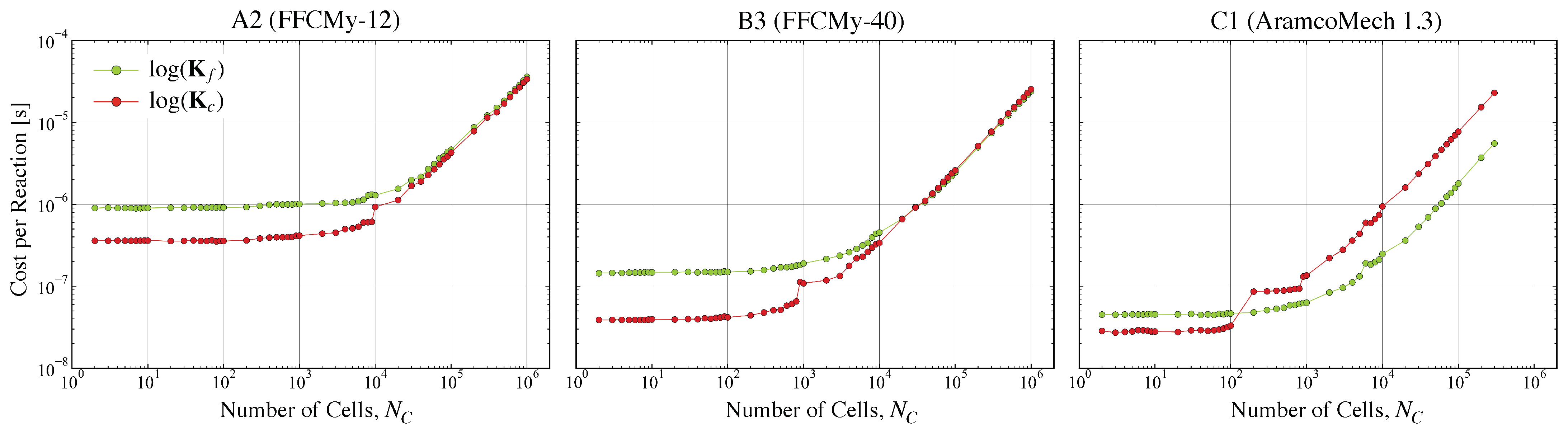
3.3. Cost of Reaction Types

The above sections described general speedup and performance trends for the GPU in light of the matrix-oriented methodology of Section 2.1. As per the classifications presented in Section 2.3, a more detailed investigation into the GPU cost of individual reaction types in the pre-saturated and saturated regimes can better illuminate both the sources of speedup behavior and the types of mechanisms that are more suited for GPU offloading.
To better isolate the GPU effects of individual routines and reaction types, the quantity of interest here is defined as the cost per reaction. The cost per reaction is measured by taking the compute time of a specific kernel (or routine composed of a set of kernels) and normalizing by the size of the subset of total reactions on which the routine acts. For example, in the case of reversible reactions, the computation of equilibrium rate constants occur on the subset of total reactions of size N R , r e v . To get a measure on the total time per reaction taken during the computation of log ( K c ) , the corresponding routine time is divided by N R , r e v . This effectively provides an averaged measure on the cost impact for individual reaction types or routines encountered in a given mechanism.
Figure 7 compares the cost per reaction for log ( K f ) and log ( K c ) routines for the three Mechanisms A2, B3, and C1. The log ( K f ) routine consists of the following: Arrhenius-based matrix multiplication (Equation (9), uses a DGEMM kernel), evaluation of third body concentrations if present (DGEMM kernel), falloff rate constant evaluations if applicable (custom kernels), and pressure-log rate constant evaluations if applicable (custom kernels). The log ( K c ) routine consists of the evaluation of Equation (9), which utilizes a first custom kernel to fill the Gibbs matrix and a second DGEMM kernel to recover the rate constants.
In the pre-saturated regime, the cost per reaction of the log ( K f ) routine consistently outweighs that of log ( K c ) . However, the behavior is different in the saturated regime as mechanism complexity grows. An interesting feature is the consistent spike in cost per reaction for log ( K c ) at the saturation points (see Figure 4) of the respective mechanisms. For the smaller mechanisms, this jump leads to a convergence in the difference between log ( K f ) and log ( K c ) costs in the saturated regime. For the large Mechanism C1, this jump at the commencement of saturation near N C = 10 2 brings the log ( K c ) cost per reaction to a higher value than the log ( K f ) cost (though not shown here, this effect is exacerbated for mechanism C2). The implication is that more complex mechanisms (as determined by N S and N R ) incur a higher penalty for log ( K c ) evaluations in the saturated regime. As such, in the case of very large mechanisms, a useful driver to design mechanisms that are more “GPU-optimal” in the saturated regime is to minimize the presence of reversible reactions, i.e., to steer the mechanism distribution towards something akin to that of C2 (see the top row of Figure 3).
Analogous costs for the three individual reaction types described in Section 2.3—standard, pressure-log, and falloff—are shown for all mechanisms in Figure 8. Recall that these reaction types modify the computation of the forward rate constant whenever applicable (i.e., they are sub-components of the log ( K f ) computation). The trends can again be characterized by behaviors in the pre-saturated and saturated regimes. For all reaction types, the cost per reaction decreases with respect to mechanism complexity, most notably for the standard reactions. This is likely the cause of the inverse trend in speedup (Figure 6) seen in the same pre-saturated regions. Further, when comparing across reaction types, standard reactions (based on the cuBLAS DGEMM) are significantly cheaper than pressure-log and falloff counterparts. This is expected due to the inherent differences in arithmetic complexity and also to the optimized implementations of the cuBLAS backend. In-line with the Roofline-derived findings of Section 3.1, mechanisms that attempt to minimize the presence of non-standard reactions are likely to achieve a greater N C -range of cost efficiency.
A prominent feature in Figure 8 is the convergence, for a specific reaction type, of all mechanism curves to the same cost per reaction in the saturated regime. This implies that, for the reaction types considered during the evaluation of log ( K f ) , the cost advantage due to mechanism complexity per reaction only applies in the pre-saturated regime. The fact that the cost per reaction mechanism curves converge here in the saturated regime is consistent with the compute time trends seen earlier in Figure 4—namely, that the overall time-to-solution in the saturated regime increase with each mechanism by the same factor of increase in N R .

3.4. Improving Speedup for Large Mechanisms

A valid concern related to the speedup in Figure 6 is the decreasing trend for Class C mechanisms. A procedure to remove this speedup deterioration for these larger mechanisms is provided here. Put briefly, the procedure relies on taking advantage of the inherent sparsity that characterizes mechanisms with high N S and N R values. This concept is first motivated by a computational budget analysis of the original routines leading to the speedups shown in Figure 6. It is then shown that a simple replacement of several problematic dense matrix multiplications with sparse counterparts very usefully recovers the “lost” speedup for the Class C mechanisms.
The computational budget, measured as the proportion of total compute time spent in the respective routines, is provided in Figure 9 for the same three mechanisms shown in Figure 7. For each mechanism and N C , the budget is split into four main components encountered during the source term computation:
  • The preprocessing routine consists of kernels that: (a) recover the primitive species mass fractions from conserved values; (b) normalize the species mass fractions in each cell to sum to unity; and (c) obtain molar concentrations from the mass fractions.
  • The forward rate constant routine for log ( K f ) computes Equation (6) along with any other non-standard reaction types that modify the forward rate (three-body, pressure-log, and falloff).
  • The equilibrium rate constant routine for log ( K c ) is outlined in Equation (9).
  • The species net production rate routine for Ω , given by Equation (2)—the cost of evaluating the net reaction rates Q n e t required to recover Ω (Equation (4))—is also included for this component.
A revealing result is that, for all mechanisms, upon entering the saturated regime, the budget is dominated by Component 4 (evaluation of the production rates). In fact, its contribution in both pre-saturated and saturated regimes grows with larger mechanisms, and the effect of saturation on the budget itself (i.e., the amount that the contribution of Component 4 changes upon entering the saturated regime) is diminished when moving from mechanism Class A to Class B and then to Class C.
Therefore, it can be concluded to good confidence that the main culprit for the diminishing speedup seen in large mechanisms in Figure 6 is derived from Component 4. This is the direct cause of prohibitive dense cuBLAS DGEMM operations involving the exceedingly large reaction matrices (matrices of size N C × N R ) found in Equations (2) and (4). Such operations involve matrix multiplications with the net, forward, and reverse stoichiometric matrices ν , ν and ν .
As alluded to above, with the contribution of Component 4 on the budget in mind, the diminishing speedups can be alleviated by recognizing that the common denominator in the prohibitive routines—the stoichiometric matrices—are predominantly sparse for large mechanisms due to the physical constraints of elementary reactions that serve as the building blocks. This effect can be visualized through the inherent correlation between mechanism sparsity, as measured by the ratio of the number of zero to total elements in the net stoichiometric matrix ν , and the N C -averaged budget contribution for component 4 (the sparsity of the net stoichiometric matrix is a conservative estimate for overall mechanism sparsity, since the forward and reverse stoichiometric matrices individually are generally more sparse). This correlation is shown in Figure 10 (left). The implication is that the primary reason for the rise in Component 4 budget, and thus the main contributor to the diminishing speedup for large mechanisms observed in Figure 6, is the sparsity. Figure 10 shows that the sparsity: (a) is quite significant (roughly 60%) even for small mechanisms; and (b) converges to nearly 100% with increasing N R .
The high sparsity for large mechanisms implies an abundance of wasted arithmetic taking place in cuBLAS-based DGEMMs, which are dense operations, used for the large reaction matrix mutiplications involving the stoichiometric matrices. Therefore, a natural step is to consider different matrix multiplication algorithms that are tailored towards sparse-dense matrix products for the larger mechanisms. This brings forward one of the most useful qualities of the matrix-oriented formulations of Section 2.1—the mechanism sparsity can be integrated into the source term computation without altering the underlying matrix-based methodology. Instead, the backend used for the matrix multiplications affected by sparsity (i.e., Equations (2) and (4)) can simply be changed from cuBLAS [24] to cuSPARSE [36], a GPU-based linear algebra library optimized for sparse computations.
The speedup achieved when moving to a sparse (driven by cuSPARSE) from a dense (driven by cuBLAS) matrix multiplication algorithm for Equation (2) is shown in Figure 10 (right). (Sparse-dense matrix multiplications are actively researched in the field of GPU computing, and there are many algorithms available. The one used here is based on the double-precision block sparse row-format matrix-multiplication (DBSRMM).) Note that the speedup shown in Figure 10 (right) compares two routines both executed on the GPU. Without delving into the specifics, the ultimate goal when switching to sparsity-based routines is that the savings in FLOPs should outweigh the new costs arising from algorithmic complexities and data retrieval. Based on these constraints, a general rule-of-thumb is to only use sparse algorithms when the sparsity is roughly above 95%. This quality is observed in Figure 10, which showcases significant matrix multiplication speedups for Mechanisms C1 (2×) and C2 (4×) in the saturated regime. Note that, when computing the sparse-to-dense speedup, the sparse compute times also include a necessary matrix transpose operation due to the fact that the cuSPARSE algorithm supports sparse-dense and not dense-sparse matrix multiplications (i.e., Equation (2) is transposed in order to use the cuSPARSE algorithm, and then the output is again transposed to conform to the data structures used in the authors’ API—all of this is taken into account when computing the speedup in Figure 10).
The translation of the results in Figure 10 into overall GPU-to-CPU speedup analogous to the original Figure 6—but instead using cuSPARSE as the backend for operations involving stoichiometric matrices—is shown in Figure 11. The results show that taking into account the mechanism sparsity alleviates the speedup deterioration seen before for the larger mechanisms of Class C. More importantly, all mechanisms regardless of size converge to similar speedup values in the saturated regime. Overall, it is encouraging that the relatively simple cuSPARSE backend modification significantly improves the GPU behavior for larger mechanisms. This warrants a more detailed analysis of the sparse algorithms themselves in relation to the stoichiometric matrix sparsity structures, since the distribution of non-zero values in the sparse matrix also affects the speedup. Such an analysis is left for future work.

4. Conclusions

In this work, a GPU investigation for a matrix-based formulation of chemical kinetics is presented. Since the target of the technique is isolated to the source term computation alone, the methods presented here are intended to supplement other related GPU-optimized techniques, such as stiff time-integration methods, that rely on the source term evaluation explicitly. Overall, the GPU performance for the species source term evaluations revealed many informative trends with regards to the effect of cell number on device saturation and speedup. Most importantly, by assessing the behavior of an ensemble of mechanisms with varying complexity, it was shown that the matrix-based method enables highly efficient GPU performance across the board, achieving near-peak performance in saturated regimes.
Of notable significance in the analysis was the classification of the different reaction types encountered in the mechanisms. This classification facilitated a detailed GPU cost and throughput analysis that revealed the impact of specific reaction types on the performance. In other words, this characterization of chemical mechanisms based on the distribution of reaction types presented in Section 2.3 provided a pathway for assessing: (a) how beneficial the matrix representation is for a particular mechanism; and (b) how the prevalence of specific reaction types can positively or negatively impact the GPU-derived speedup. The main reason for introducing the reaction-type classification was to bring forward the idea that, in the determination of GPU speedup, mechanism species and reaction numbers are not the only factors; the complexity of the individual reactions themselves also plays an important role. A common theme which came from this analysis was the tendency of the GPU to favor simplicity above all else, which conforms to the single-instruction multiple-thread nature of the hardware—the implication is that designing larger mechanisms with more standard, irreversible reactions is more favorable in GPU settings.
A prominent feature of the matrix-based formulation is its ability to intrinsically support sparse algorithms. In particular, it was found that the high amounts of sparsity characterizing larger chemical mechanisms could be directly taken advantage of by changing the matrix multiplication backend from cuBLAS to cuSPARSE routines. This quality brought forward an advantageous aspect of the matrix-oriented formulations of Section 2.1; namely, the mechanism sparsity can be integrated into the source term computation without altering the underlying matrix-based methodology. In summary, taking into account the mechanism sparsity alleviated the speedup deterioration seen larger mechanism classes.
The results of this study open many pathways for future work. For example, the performance-related findings discussed here can be used to directly translate, or even reduce, existing mechanisms into more GPU optimal descriptions. Further, the findings related to sparsity warrants a more detailed analysis of the sparse algorithms themselves in relation to the stoichiometric matrix structures, since the distribution of non-zero values in the sparse matrix also affects the speedup. Additionally, the opportunities presented by neural network interpretations (as presented in Section 2.1 and Appendix A) are promising routes by which even more computational gain can be extracted.

Author Contributions

Conceptualization, S.B. and V.R.; methodology, S.B. and V.R.; software, S.B. and V.R.; validation, S.B.; formal analysis, S.B. and V.R.; investigation, S.B. and V.R.; resources, S.B. and V.R.; data curation, S.B.; writing—original draft preparation, S.B.; writing—review and editing, S.B. and V.R.; visualization, S.B.; supervision, V.R.; project administration, V.R.; funding acquisition, S.B. and V.R. All authors have read and agreed to the published version of the manuscript.

Funding

This research received no external funding.

Institutional Review Board Statement

Not applicable for studies not involving humans or animals.

Informed Consent Statement

Not applicable for studies not involving humans.

Data Availability Statement

The data presented in this study are available on request from the corresponding author.

Acknowledgments

This research used resources of the Oak Ridge Leadership Computing Facility, which is a DOE Office of Science User Facility, supported under Contract DE-AC05-00OR22725.

Conflicts of Interest

The authors declare no conflict of interest.

Appendix A. Substitution with Approximate Artificial Neural Networks

In Section 2.1, the matrix based formulations of the kinetics routines are exact and perform at high efficiency on GPUs as they stand. The ANN interpretations of these exact formulations, however, illuminate pathways where additional computational efficiency can be extracted by utilizing so-called “approximate ANNs” as drop-in replacements for the “exact ANN” architectures described in Figure 1. At the cost of perfect accuracy, such replacements allow for direct control over computational cost through a customized ANN architecture whose parameters are trained with data. The end goal is that the execution time of the approximate ANN should be faster than the exact ANN counterparts (to clarify, “exact ANN” here refers to the exact matrix-based formulations of Section 2.1).
Many pathways to this end are available. For the sake of demonstrating how this technique can be applied, the replacement of the exact ANN for the logarithm of the equilibrium rate constant (Figure 1c) with an approximate ANN counterpart is explored. In other words, in this demonstration, the modeling goal of the approximate ANN is to recover accurate representations of log ( K c ) and not the species production rates Ω directly.
Narrowing the approximate ANN scope to log ( K c ) brings forward two key advantages. The first is that the equilibrium rate constants do not depend on the species concentrations, but rather only on nonlinear functions of temperature. This means that the sampling of an N S -dimensional phase space to develop a training dataset—a huge bottleneck in many existing ANN-based source term modeling techniques that becomes prohibitive for large mechanisms—is not required in the training phase. The second advantage is that known physical constraints to recover the source terms, such as the relationship between concentrations and net reaction rate (Equation (4)), as well as Arrhenius forms for the forward rate (Equation (6)), are preserved in the overall computation, ensuring high accuracy and physical consistency. Additionally, the exact ANN architecture for log ( K c ) (shown in Figure 1c) is complex enough to warrant a reduction based on an approximate ANN—there is more than one layer in the exact form, which is not the case for the forward rate constant architecture. This is crucial because the design of the approximate ANN must be driven by reducing computational effort. In other words, the exact ANN form should serve as an upper bound for the computational complexity (in terms of a cost metric such as FLOPs, for example) of the approximate ANN.
In general, an ANN layer takes the following form:
X l + 1 = σ l ( X l W l + B l ) , l = 0 , , N L ,
where X l is the layer input, X l + 1 is the layer output, W l is the weight matrix, B l is the bias vector, σ is an activation function, and N L is the total number of hidden layers. Note that, unlike in Section 2.1, the parameters (weights/biases) are assumed unknown in this setting and are found through a training procedure. As with the exact formulations, the leading dimension (batch size) for these input and output matrices is N C . For a given N L , the hidden layer dimension N H (or number of neurons per hidden layer) is assumed to be fixed for the sake of this walk-through, but this does not have to be the case in general.
The ANN input is X 0 R N C × N i n and the output is X N L + 1 R N C × N R = log ( K c ˜ ) . The main task is to train the ANN such that log ( K c ˜ ) log ( K c ) . The only restrictions are that the input features are functions of temperature and the output dimensionality is N R (assuming without loss of generality that all reactions in the mechanism are reversible). To highlight key points, two examples of approximate ANN architectures are shown in Figure A1. Architecture 1 uses the same input features as the exact ANN but allows for variation N L and N H (referred to as the modified Gibbs neurons). Architecture 2 is similar but only utilizes one input feature, namely log ( T ) .
Nonlinearity is imposed in both architectures through the activation functions σ l . In Architecture 1, since several functions of temperature are already included in the input, a simple rectified linear unit (relu) activation function can be used:
x R , σ l ( x ) = relu ( x ) = max ( 0 , x ) .
On the other hand, since Architecture 2 utilizes only log ( T ) in the input layer, the more expensive exponential linear unit (elu) activation can be used [37] to allow the model to extract dependence on powers of T as needed during the training process:
x R , σ l ( x ) = elu ( x ) = x if x 0 , e x 1 if x < 0 .
In the above scenario, it is reasonable to expect that the computational advantage offered by the smaller input size of Architecture 2 is offset by the more expensive activation function. In light of this, Architecture 2 can be modified to use the relu activation, although this lessens the expressive power of the ANN. For example, with only log ( T ) as the input, an ANN using Equation (A2) throughout cannot easily represent a function composed of polynomials of T; its architecture must be modified to at least include T itself as an additional input (akin to Architecture 1). Moreover, Architecture 2 can be modified to include 1 / T as an additional input, and Architecture 1 can be modified to remove the higher order temperature terms ( T 2 , T 3 , and T 4 ). In the tests conducted by the authors, such modifications were found not to significantly affect the end results—all variations were sufficiently accurate when trained until convergence using a mean-squared error loss function on log ( K c ) .
Figure A1. Illustrations of ANN representations for log ( K c ) : (Left) exact ANN (same as Figure 1c); (Middle) approximate ANN, Architecture 1; and (Right) approximate ANN, Architecture 2. The number of modified Gibbs neurons changes through N H and N L ( N H = 2 here for illustrative purposes).
Energies 14 02710 g0a1
The key takeaways are that the formulation of the approximate ANN for the equilibrium constants involves reductions and re-castings of the exact form in a few major aspects: (1) the re-interpretation of the exact Gibbs neurons (Figure A1, left) into the modified Gibbs neurons (Figure A1, middle and right); (2) the fact that the approximate ANN evaluation is not treated in distinct temperature partitions (in the exact setup of Equation (9), the polynomial coefficients for a particular species, which are interpreted as the weights, are temperature-dependent whereas the approximate ANN weights are not); and (3) the customized form of the input layer and nonlinearity in the approximate ANN. Such reductions and changes are necessary to motivate the approximate ANN from a computational efficiency and simplicity aspect with respect to the exact form.
The above concepts were presented in the context of replacing the equilibrium rate constant with an approximate ANN, but the same techniques can be applied for other components such as the forward rate constant. For example, using an approximate ANN to consolidate the standard, falloff, and pressure-log forward rate constant computations into a single matrix multiplication operation could be a promising application of the technique.

Appendix B. Verification of GPU Implementation

As a simple verification for the GPU implementation, scatter plots for the source terms as compared with the baseline CPU Cantera implementation (obtained from the function call getNetProductionRates) are shown in Figure A2a,b for mechanisms B3 and C2, respectively; the results are analogous for all other mechanisms. The source terms were computed by randomly sampling ensembles of species mass fractions, temperatures, and pressures. Additionally, ignition delay time verification for mechanism B3, which contains all the mechanism complexity considered in this work (i.e., the distribution, as shown in Figure 3, contains reversible, irreversible, standard, falloff, and pressure-log reactions), is shown in Figure A2c. Cantera and GPU-based mass fraction time series profiles obtained from a mechanism B3 ignition simulation for several intermediary species are also provided in Figure A2d,e.
Figure A2. (a) Scatter plots comparing GPU (y-axis) and CPU-based Cantera (x-axis) species source term values for mechanism B3. Dashed black line represents the exact solution. (b) Same as (a), but for mechanism C2. (c) Constant-volume ignition delay times for mechanism B3 using the GPU formulation (squares) and Cantera (circles). For the initial condition, an ethylene-air mixture was used at an equivalence ratio of unity with an initial pressure of 10 atm. (d) Intermediary species profiles from a constant-volume ignition simulation (same conditions as specified in (c) with initial temperature of 1800 K) using the GPU implementation (dashed colors) and Cantera (solid black). (e) Same as (d), but in logarithmic scale on the y-axis.
Energies 14 02710 g0a2
In all cases, the matrix-based GPU implementation of Section 2.1 and the CPU-based Cantera results are indistinguishable. It should be noted that, since the equations are programmed differently in terms of algorithmic implementations and the compilers vary, some small expected truncation-related errors that are not apparent in the scatter plots do appear; however, these errors are on the order of machine precision and do not propagate.

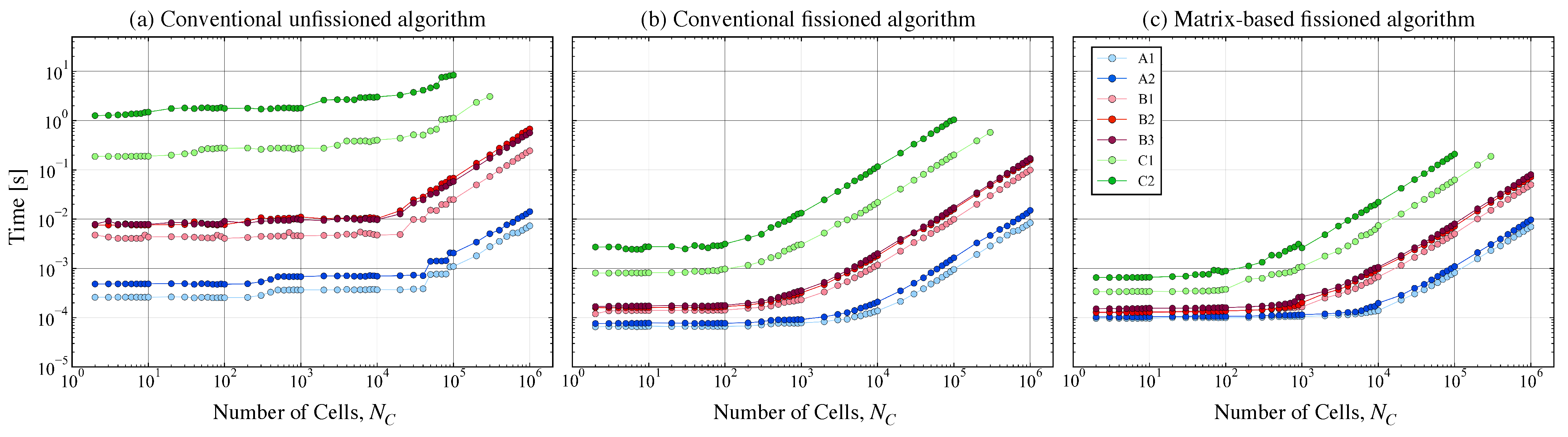
Appendix C. Performance Comparison with Non-Matrix Approaches

The results presented in Section 3 focus solely on the GPU performance of the matrix-based formulations. The discussion below, on the other hand, provides comparisons between the matrix-based approach and two baseline, more conventional approaches that do not utilize the matrix formulations. The algorithmic details of these conventional methods are provided further below. Ultimately, through a direct comparison of evaluation times, the primary goal is to isolate the gain in performance when moving from a more conventional kinetics offloading approach to the matrix-based approach. The secondary goal is to present clearly the GPU offloading algorithms, for both matrix-based and conventional approaches, in terms of the organization of GPU kernels.
It should be noted that the definition of “conventional” is less obvious when dealing with GPUs. This is because GPU offloading introduces the kernel launch aspect as an additional degree of complexity in the algorithm design: one has to decide how many GPU kernels to break the function evaluation into. In this vein, the so-called kernel “fissioning” process must be established. Fissioning refers to the way in which a function evaluation offloaded to a GPU can be broken down into a set of smaller function evaluations to expose more parallelism. Essentially, for a given complex function with many internal stages such as the source term evaluation considered in this work, the unfissioned approach casts the function as a single very large GPU kernel with one principle vectorization direction (i.e., one kernel to replace the main loop over the number of cells, for example), whereas the fissioned approach breaks the function down into a set of smaller GPU kernels to potentially expose multiple vectorization directions and higher thread concurrency (i.e., a given kernel in the fissioned approach may replace a sub-function comprised of a nested for loop that iterates over both cells and species). As detailed below, the matrix-based algorithm profiled in Section 3.1 by design adopts the fissioned approach.
Diagrams for the three GPU algorithms are provided in Figure A3. Figure A3a is the conventional unfissioned algorithm, Figure A3b is the conventional fissioned algorithm, and Figure A3c is the matrix-based fissioned algorithm. All three approaches utilize the same inputs and produce the same output Ω (see Section 2.1). The general inputs are the thermodynamic data for each cell (mass fraction, temperature, and density) and chemical mechanism information (stoichiometric matrices, reaction parameters, reaction type indicators, polynomial coefficients, etc.). The key difference is that these inputs are distributed over several kernel launches in the fissioned approach (Figure A3b,c), whereas, in the unfissioned approach (Figure A3a), all inputs are fed into one kernel. Additional relevant details for each approach are discussed below.
The algorithm in Figure A3a is labeled as “conventional” because it does not operate in the logarithm space—it evaluates the source term using the standard equations. Further, it is “unfissioned” because the source term evaluation is represented as a single large kernel. More precisely, Figure A3a captures the effect of threading a direct source term function evaluation over the number of cells, N C , without taking advantage of the reaction and species matrix data structures outlined in Section 2.2. Instead, on each function call, each thread in this algorithm operates on a single cell and loops through every reaction to accumulate the source term contribution for the set of species involved in that particular reaction. As such, within the reaction loop over N R , there are several species loops over N S (red bullets in Figure A3a) that represent this accumulation of species information (reductions) by means of the stoichiometric matrices. Overall, Figure A3a is a useful baseline because it resembles the impact of sending a CPU-type approach directly to the GPU without any underlying algorithmic changes. Note that Figure A3a is demonstrative and is not expected to be GPU-optimal, because: (1) the kernel launch overhead is high; and (2) there are many distributed global memory access points and conditional statements scattered throughout the kernel.
Figure A3. (a) The conventional unfissioned algorithm. The gray box denotes the scope of the CUDA kernel. The notation “1D grid over N C ” means the kernel is launched on a one-dimensional grid of thread blocks defined by the number of cells N C . The yellow box denotes the per-thread reaction loop. The steps marked in red denote locations where a loop over the number of species N S is required (arithmetic in a species loop is only performed for a species involved in the given reaction). (b) The conventional fissioned algorithm to be read top-down. Each gray box denotes a single kernel launch. For each kernel, the arrow indicates the dimensionality of the kernel launch (i.e., vectorization directions). (c) Same as (b), but instead shows the matrix-based fissioned algorithm as profiled in Section 3.1 (the primary contribution of this work). Black stars denote kernels that can be evaluated using cuBLAS and red stars denote kernels that allow for cuSPARSE calls if desired (see Section 3.4).
Energies 14 02710 g0a3
The algorithms in Figure A3b,c are fissioned representations of Figure A3a—the single large kernel of Figure A3a has been effectively decomposed into a set of smaller kernels, each playing an isolated role in the source term evaluation. The approach in Figure A3b is the conventional analog to the matrix-based approach in Figure A3c: the multidimensional threading advantages provided by the data structures in Section 2.2 are retained, with the key difference being the matrix-based calculations (i.e., GEMMs) for the rate constants and net production rate evaluations are not utilized. In summary, the advantages of the matrix-based approach (Figure A3c) can be assessed by directly comparing its performance with the Figure A3b algorithm, and the advantages of the fissioning approach for this particular problem can be assessed by comparing the algorithms in both Figure A3b,c with that of Figure A3a.
Figure A4 shows the GPU source term evaluation times obtained from the respective algorithms in Figure A3. Note that the matrix-based algorithm times in Figure A4c come from the dense cuBLAS GEMM routines and are identical to those shown previously in Figure 4.
Figure A4. GPU source term evaluation times for: (a) the conventional unfissioned algorithm; (b) the conventional fissioned algorithm; and (c) the matrix-based fissioned algorithm.
Energies 14 02710 g0a4
It is apparent that the conventional unfissioned algorithm (Figure A4a) observes significantly altered saturation and compute trends when compared to the fissioned counterparts. Due to the fact each thread directly iterates over a reaction loop, the unfissioned algorithm is characterized by roughly vertical shifts of the compute time curve in proportion to the increase in N R for the entire set of N C , not just in the saturated regime. This ultimately means that the unfissioned algorithm becomes prohibitively slow as the mechanism size increases for all values of N C . This is due not only to the increased arithmetic, but also to the increase in inefficient global memory transactions performed by each thread as the mechanism size increases. For example, for the class-C mechanisms, Figure A4a shows a smaller relative increase in compute time with an increase in N C —this implies that the execution time is dominated by inefficient memory accesses and high kernel launch overhead (i.e., non-arithmetic operations). The deviation of the saturation point trends in with respect to the fissioned algorithms in Figure A4b,c likely stems from the same cause, but requires further investigation.
The trends in Figure A4b,c are very similar—the characteristic approach to the saturation point is retained by the conventional fissioned algorithm. The effect of transitioning from the conventional fissioned approach to the matrix-based fissioned approach is better visualized in Figure A5, which shows the speedup provided by the matrix formulation (time in Figure A4b divided by time in Figure A4c). The speedup curves show how the matrix-based approach gives increasingly higher performance boosts as both the mechanism size and number of cells increases. Interestingly, for the smaller class-A mechanisms, the conventional non-matrix algorithm is more efficient (speedup of 0.5 , or roughly twice as fast) in the pre-saturated regime. This likely comes from the additional expensive arithmetic operations, such as element-wise exponentiations and logarithms, present in the matrix-form that are avoided in the conventional evaluation—essentially, for cases where the speedup is below unity, the cost of these additional complexities is not offset by the efficiency of the linear algebra routines. As the GPU saturates, this effect is diminished, and the performance boost provided by the matrix-based algorithm is recovered even for small mechanisms. Note that the speedups shown in Figure A5 do not include the effect of cuSPARSE acceleration for large mechanisms. This effect can be derived directly from the analogous curves in Figure 10 (right)—essentially, the performance boost provided by the matrix-based algorithm when taking sparsity into account provides roughly an additional factor of 2–4 speedup for large mechanisms.
Figure A5. Speedup provided by the matrix-based fissioned algorithm over the conventional fissioned counterpart (evaluation times in Figure A4b divided by times in Figure A4c).
Energies 14 02710 g0a5

References

  1. Hochgreb, S. Mind the gap: Turbulent combustion model validation and future needs. Proc. Combust. Inst. 2019, 37, 2091–2107. [Google Scholar] [CrossRef] [Green Version]
  2. Raman, V.; Hassanaly, M. Emerging trends in numerical simulations of combustion systems. Proc. Combust. Inst. 2019, 37, 2073–2089. [Google Scholar] [CrossRef] [Green Version]
  3. Pitsch, H. Large-eddy simulation of turbulent combustion. Annu. Rev. Fluid Mech. 2006, 38, 453–482. [Google Scholar] [CrossRef] [Green Version]
  4. Chen, J.H. Petascale direct numerical simulation of turbulent combustion—Fundamental insights towards predictive models. Proc. Combust. Inst. 2011, 33, 99–123. [Google Scholar] [CrossRef]
  5. Jaravel, T.; Riber, E.; Cuenot, B.; Pepiot, P. Prediction of flame structure and pollutant formation of Sandia flame D using Large Eddy Simulation with direct integration of chemical kinetics. Combust. Flame 2018, 188, 180–198. [Google Scholar] [CrossRef]
  6. Mueller, M.E. A computationally efficient turnkey approach to turbulent combustion modeling: From elusive fantasy to impending reality. In Proceedings of the AIAA Scitech 2019 Forum, San Diego, CA, USA, 7–11 January 2019; p. 0994. [Google Scholar]
  7. Pope, S.B. Turbulent Flows; Cambridge University Press: Cambridge, UK, 2000. [Google Scholar]
  8. Raman, V.; Pitsch, H. A consistent LES/filtered-density function formulation for the simulation of turbulent flames with detailed chemistry. Proc. Combust. Inst. 2007, 31, 1711–1719. [Google Scholar] [CrossRef]
  9. Menon, S.; Kerstein, A.R. The linear-eddy model. In Turbulent Combustion Modeling; Springer: Dordrecht, The Netherlands, 2011; pp. 221–247. [Google Scholar]
  10. Pope, S. Computationally efficient implementation of combustion chemistry using in situ adaptive tabulation. Combust. Theory Model. 1997, 1, 41–63. [Google Scholar] [CrossRef]
  11. Tonse, S.R.; Moriarty, N.W.; Brown, N.J.; Frenklach, M. PRISM: Piecewise reusable implementation of solution mapping. An economical strategy for chemical kinetics. Isr. J. Chem. 1999, 39, 97–106. [Google Scholar] [CrossRef] [Green Version]
  12. Christo, F.; Masri, A.; Nebot, E.; Pope, S. An integrated PDF/neural network approach for simulating turbulent reacting systems. Symp. (Int.) Combust. 1996, 26, 43–48. [Google Scholar] [CrossRef]
  13. Sen, B.A.; Menon, S. Turbulent premixed flame modeling using artificial neural networks based chemical kinetics. Proc. Combust. Inst. 2009, 32, 1605–1611. [Google Scholar] [CrossRef]
  14. Kempf, A.; Flemming, F.; Janicka, J. Investigation of lengthscales, scalar dissipation, and flame orientation in a piloted diffusion flame by LES. Proc. Combust. Inst. 2005, 30, 557–565. [Google Scholar] [CrossRef]
  15. Owoyele, O.; Kundu, P.; Ameen, M.M.; Echekki, T.; Som, S. Application of deep artificial neural networks to multi-dimensional flamelet libraries and spray flames. Int. J. Engine Res. 2020, 21, 151–168. [Google Scholar] [CrossRef]
  16. Barwey, S.; Prakash, S.; Hassanaly, M.; Raman, V. Data-driven Classification and Modeling of Combustion Regimes in Detonation Waves. Flow Turbul. Combust. 2020, 106, 1065–1089. [Google Scholar] [CrossRef]
  17. Reed, D.A.; Dongarra, J. Exascale computing and big data. Commun. ACM 2015, 58, 56–68. [Google Scholar] [CrossRef]
  18. Nickolls, J.; Dally, W.J. The GPU computing era. IEEE Micro 2010, 30, 56–69. [Google Scholar] [CrossRef]
  19. Niemeyer, K.E.; Sung, C.J. Recent progress and challenges in exploiting graphics processors in computational fluid dynamics. J. Supercomput. 2014, 67, 528–564. [Google Scholar] [CrossRef] [Green Version]
  20. Niemeyer, K.E.; Sung, C.J. Accelerating moderately stiff chemical kinetics in reactive-flow simulations using GPUs. J. Comput. Phys. 2014, 256, 854–871. [Google Scholar] [CrossRef] [Green Version]
  21. Curtis, N.J.; Niemeyer, K.E.; Sung, C.J. Using SIMD and SIMT vectorization to evaluate sparse chemical kinetic Jacobian matrices and thermochemical source terms. Combust. Flame 2018, 198, 186–204. [Google Scholar] [CrossRef] [Green Version]
  22. Sewerin, F.; Rigopoulos, S. A methodology for the integration of stiff chemical kinetics on GPUs. Combust. Flame 2015, 162, 1375–1394. [Google Scholar] [CrossRef]
  23. Pérez, F.E.H.; Mukhadiyev, N.; Xu, X.; Sow, A.; Lee, B.J.; Sankaran, R.; Im, H.G. Direct numerical simulations of reacting flows with detailed chemistry using many-core/GPU acceleration. Comput. Fluids 2018, 173, 73–79. [Google Scholar] [CrossRef] [Green Version]
  24. cuBLAS, The CUDA Basic Linear Algebra Subroutine Library. NVIDIA Corporation. 2021. Available online: https://docs.nvidia.com/cuda/cublas/index.html (accessed on March 2021).
  25. Poinsot, T.; Veynante, D. Theoretical and Numerical Combustion; RT Edwards, Inc.: Philadelphia, PA, USA, 2005. [Google Scholar]
  26. Goodwin, D.G.; Moffat, H.K.; Speth, R.L. Cantera: An Object-Oriented Software Toolkit for Chemical Kinetics, Thermodynamics, and Transport Processes. 2017. Available online: https://www.cantera.org (accessed on March 2021).
  27. Kee, R.J.; Rupley, F.M.; Miller, J.A. Chemkin-II: A Fortran Chemical Kinetics Package for the Analysis of Gas-Phase Chemical Kinetics; Technical Report; Sandia National Lab.(SNL-CA): Livermore, CA, USA, 1989. [Google Scholar]
  28. Mueller, M.; Kim, T.; Yetter, R.; Dryer, F. Flow reactor studies and kinetic modeling of the H2/O2 reaction. Int. J. Chem. Kinet. 1999, 31, 113–125. [Google Scholar] [CrossRef]
  29. Xu, R.; (Stanford University, 440 Escondido Mall, Stanford, CA, USA); Wang, H.; (Stanford University, 440 Escondido Mall, Stanford, CA, USA). Reduced Reaction Models for Methane and Ethylene Combustion. Personal communication, 2020. [Google Scholar]
  30. Smith, G.; Tao, Y.; Wang, H. Foundational Fuel Chemistry Model Version 1.0 (FFCM-1). 2016. Available online: http://nanoenergy.stanford.edu/ffcm1 (accessed on August 2020).
  31. Chemical-Kinetic Mechanisms for Combustion Applications. San Diego Mechanism web page, Mechanical and Aerospace Engineering (Combustion Research), University of California at San Diego. 2016. Available online: http://web.eng.ucsd.edu/mae/groups/combustion/mechanism.html (accessed on August 2020).
  32. Metcalfe, W.K.; Burke, S.M.; Ahmed, S.S.; Curran, H.J. A hierarchical and comparative kinetic modeling study of C1–C2 hydrocarbon and oxygenated fuels. Int. J. Chem. Kinet. 2013, 45, 638–675. [Google Scholar] [CrossRef]
  33. Mehl, M.; Pitz, W.J.; Westbrook, C.K.; Curran, H.J. Kinetic modeling of gasoline surrogate components and mixtures under engine conditions. Proc. Combust. Inst. 2011, 33, 193–200. [Google Scholar] [CrossRef] [Green Version]
  34. The Nvprof Profiling Tool. NVIDIA Corporation. 2021. Available online: https://docs.nvidia.com/cuda/profiler-users-guide (accessed on March 2021).
  35. Williams, S.; Waterman, A.; Patterson, D. Roofline: An insightful visual performance model for multicore architectures. Commun. ACM 2009, 52, 65–76. [Google Scholar] [CrossRef]
  36. cuSPARSE, The CUDA Sparse Matrix Library. NVIDIA Corporation. 2021. Available online: https://docs.nvidia.com/cuda/cusparse/index.html (accessed on March 2021).
  37. Clevert, D.A.; Unterthiner, T.; Hochreiter, S. Fast and accurate deep network learning by exponential linear units (elus). arXiv 2015, arXiv:1511.07289. [Google Scholar]
Figure 1. Illustrations of ANN-based formulations for N C = 1 , N S = 4 , and N R = 8 . Since N C = 1 , input/outputs are vectors and cell indices are ignored. (a) Schematic of Equations (2) and (4). Exponential activation functions are used to produce forward/reverse rates. (b) Schematic of Arrhenius layer for forward rate constant (Equation (6)), which is interpreted as a bias term for the output of the forward rate layer in (a) (see Equation (4)). (c) Schematic of Gibbs layer equilibrium constant (Equation (11)). The schematics in both (b,c) produce the logarithm of the reverse rate constant, which is interpreted as a bias term for the output of the reverse rate layer in (a) (see Equation (4)).
Energies 14 02710 g001
Figure 2. (a) Interpretations of a matrix in column major (left) and row major (right) formats. The gray shapes within the matrices show the storage method as a stacking of N R column vectors (for column major) or N C row vectors (for row major). (b) Decomposition of a reaction matrix into N R , i r v irreversible and N R , r e v reversible sub-matrices, each with another set of sub-matrices corresponding to standard, falloff, and pressure-log reaction types.
Energies 14 02710 g002
Figure 3. Reaction distributions shown as pie charts for the mechanisms listed in Table 1. The top row shows proportions of reversible and irreversible reactions, whereas the bottom row shows proportions of standard, falloff, and pressure-log reactions. Indicated for each wedge is the proportion (reaction number normalized by total number of reactions) as a percentage, and the absolute reaction number in parentheses. The significant difference in the reaction distribution for C2 with respect to reversibility is due to the fact that most of the reversible reactions were parameterized with Arrhenius expressions for both forward and reverse components (see the introductory comments of Section 2.3).
Energies 14 02710 g003
Figure 4. Absolute compute time (time-to-solution) as a function of cell number N C for the GPU evaluation of the species source terms for the mechanisms listed in Table 1. Saturation points for each mechanism group are indicated by the black arrows.
Energies 14 02710 g004
Figure 5. (a) Roofline model for mechanism B3 for all kernels encountered during the source term computation. Each marker represents a unique kernel evaluated for the number of cells N C indicated by its color. (b) Roofline model for the DGEMM kernel. (c) Roofline model for the Troe falloff kernel. In (b,c), the different colors represent different mechanisms (see Table 1) and the distribution of points of the same color comes from the various N C values.
Energies 14 02710 g005
Figure 6. (Left) GPU-derived speedup in log-scale with respect to the Cantera-based CPU baseline for all mechanisms listed in Table 1. (Right) Same as left but with linear-scale in the y-axis.
Energies 14 02710 g006
Figure 7. Cost per reaction for forward rate constant ( log ( K f ) ) and equilibrium constant ( log ( K c ) ) routines as a function of N C for: Mechanism A2 (left plot); Mechanism B3 (middle); and Mechanism C1 (right).
Energies 14 02710 g007
Figure 8. Cost per reaction for all mechanisms for: standard reactions (left); pressure-log reactions (middle); and falloff reactions (right). See Table 1 for mechanism information.
Energies 14 02710 g008
Figure 9. Computational budget (routine time normalized by total compute time) for the preprocessing routine (Component 1, blue curve), forward rate constant routine (Component 2, green curve), equilibrium rate constant routine (Component 3, red curve), and net production rate routine (Component 4, yellow curve). The results are shown for the same three mechanisms as in Figure 7.
Energies 14 02710 g009
Figure 10. (Left) Mechanism sparsity and average component 4 budget (the budget corresponding to the evaluation of Equations (2) and (4)) versus number of reactions N R . (Right) Dense (cuBLAS) to sparse (cuSPARSE) matrix multiplication speedup (dense compute times divided by sparse compute times) for evaluating Equation (2) shown for all mechanisms with respect to N C . See Table 1 for mechanism information.
Energies 14 02710 g010
Figure 11. Updated GPU-to-CPU speedup values when taking into account the mechanism sparsity (analogous to Figure 6).
Energies 14 02710 g011
Table 1. List of mechanisms used throughout this work arranged in ascending order of N R . They are grouped into three classes based on N R for ease of reference. Class A is for smaller mechanisms ( N R = O ( 10 ) ), Class B for medium-sized mechanisms ( N R = O ( 100 ) ), and Class C for large mechanisms ( N R = O ( 1000 ) ). Note that the mechanism labeled C1 is unrelated to the jet fuel of the same name.
ClassReferenceDescription N S N R
A1Mueller et al. [28]Hydrogen/Air921
A2FFCMy-12 [29,30]Methane/Oxygen1238
B1FFCMy-30 [29]Ethylene/Air30231
B2UCSD [31]Hydrogen/Air57268
B3FFCMy-40 [29]Ethylene/Air41361
C1AramcoMech 1.3 [32]2531542
C2LLNL [33]6544846
Publisher’s Note: MDPI stays neutral with regard to jurisdictional claims in published maps and institutional affiliations.

