Multi-Point-of-View Energy Loss Analysis in a Refuse Truck Hydraulic System

Abstract

In recent years, much research has focused on reducing the power consumption of mobile hydraulic machines due to rising fuel costs, regulations on combustion engine emissions and the need to reduce the size and weight of the storage devices in hybrid drives. Current approaches to improve the energy efficiency of a hydraulic system can be classified into four basic groups: reduction of the energy demand, recovery of part of the supplied energy (ERS systems), regeneration of part of the supplied energy and reuse of the recovered and regenerated energy (hybrid systems). Today’s mobile hydraulic systems are often complex, perform different tasks and work under different load conditions, which makes it difficult to analyse energy losses. A study of the energy losses of a hydraulic system from different points of view, such as an energy balance for a complete machine cycle, an analysis of the individual cycle phases and a power analysis for the different operation quadrants of the actuators, can give an global picture of the energy losses, being very useful to rate its energy efficiency, identify main power losses and decide which of the different energy-saving techniques to apply. This paper describes the data collection process, its analysis from various points of view and the summary of the results in easy to understand charts as useful tools to identify and quantify the main energy losses. Only system architecture losses are considered. Losses in the ICE engine or the electric motor, hydraulic pump losses and mechanical losses are outside the scope of this study.

1. Introduction

Although energy-efficient hydraulics has attracted considerable research interest over the last decades, the efficiency of today´s mobile hydraulic systems is often still relatively low, even in those machines where efficient and well-sized individual components are used.

Current approaches to improve the energy efficiency of a hydraulic system can be classified into four basic groups: reduction of the energy demand, recovery of part of the supplied energy (ERS systems), regeneration of part of the supplied energy and reuse of the recovered and regenerated energy (hybrid systems).

Table 1. Comparison of different methods to reduce the energy demand of a hydraulic system.

Method	Throttling Losses	Recovery Potential	Cost
Load sensing (LS)	High	Low	Low
Independent metering (IM)	Medium	High	Medium
Digital hydraulics (DH)	Medium	High	Medium
Displacement control (DC)	Low	High	High
Electrohydraulic actuators (EHA)	Low	High	High
Hydraulic transformers (HT)	Low	High	High
Common rail (CPS)	Medium	High	Medium

shows different solutions for reducing the energy demand. In most current commercial applications today, the system architecture is based on one or several variable displacement pumps, each feeding several actuators through a proportional valve, using the concept of load-sensing (LS), a technology from the 1970s. The main weaknesses of this technology are the high throttling losses and the fact that the pump pressure must match the pressure demanded by the highest loaded actuator plus an additional LS overpressure, typically 10 to 30 bar.

Overviews of different approaches to reduce energy losses can be found in [1,2,3]. Examples of variations of the traditional load-sensing architecture to improve its efficiency are the flow-on-demand load-sensing (FOD) proposed in [4] and the electronic load-sensing (ELS) shown in [5]. Some LS variations are investigated in [6,7] on a medium-sized agricultural tractor.

The basis of the independent metering (IM) is to separate the control of the meter-in and meter-out ports of the actuator. Some examples can be found in [8,9]. The results of a research project on hydraulic hybrid machines and independent metering are presented in [10].

Hydraulic system digitalization (DH) is usually applied to valves, replacing traditional proportional valves with high-speed on/off valves [11], but there are also applications on pumps, i.e., switching on/off individual pistons in a radial piston pump, as shown in [12], and in actuators, i.e., the multi-chamber cylinder presented in [13].

In displacement control (DC) architecture, a variable displacement pump/motor unit controls the motion of each actuator. An example of its use in an excavator can be found in [14].

Electrohydraulic actuators (EHA) are based on a variable speed electric motor driving a displacement pump, which is directly coupled to the actuator, i.e., a cylinder, combining the specific advantages of electro-mechanical screw drives, such as high-energy efficiency and low noise emission, with the benefits of the hydrostatic drives, which include robustness and the precise handling of large forces. An overview with different examples is presented in [15].

Hydraulic transformers (HT) convert hydraulic input power into hydraulic output power, adapting pressure and flow to the actuator demand without throttling losses. An application of this technology for a wheel loader is shown in [16].

In constant pressure systems (CPS), also known as common rail systems, there are at least one high pressure line and one low pressure line, each at a constant and different pressure level, with the actuators connected between the two lines. In [17], their possibilities in mobile hydraulic machines are studied. A design with a third intermediate pressure line is presented in [18]. In addition, different energy recovery systems are also proposed in [19,20].

Before deciding the best architecture for a given system, it is necessary however to identify and quantify the sources of energy loss, which is often difficult due to the complexity of the systems and the variability of the operating conditions [21]. In this sense, a multi-point-of-view analysis is a useful tool and the main contribution of this work.

The available literature only performs energy balances from a single point of view. Generally, it is a matter of deducing an approximate overall performance of the machine or obtaining a picture of the energy balance. Therefore, some information is missing. This study proposes to sequentially combine a series of methods (analysis of the system from different points of view), basically: energy balance for a complete machine cycle (Sankey diagram), analysis of the different phases of the cycle and power analysis for the different operation quadrants (4-quadrant power map). This information can be the starting point for optimizing the hydraulic system from an energetic point of view. More suitable, better-sized, better-controlled components can be chosen, or alternatively innovative architectures can be implemented.

A Sankey plot resulting from the calculation of the energy losses in different parts of the circuit for a particular working cycle shows the energy flows, giving information on where the losses are located and what their magnitude is. The authors of [22] use the Sankey diagram as an energy balance to compare alternative solutions for hydraulic excavators. Other Examples of the use of Sankey diagrams can be found in [23,24] and [25,26]. This information can be supplemented with pie charts showing more detailed information, as can be seen in [25,26,27].

Plotting the sum of the power demanded by the actuators versus time for a complete cycle, considering positive the resistive power and negative the assistive power, clearly shows the amount of energy that can potentially be reused, as shown in [22,23].

Furthermore, dividing the cycle into different phases considering the actuators working simultaneously and analysing the different phases, helps to quantify the percentage of losses associated with the parallel operation of the actuators.

Analysis of actuator quadrant performance showing the results in a 4-quadrant power map takes into account the direction of force and speed, identifying whether the loads are resistive or assistive. It also makes it possible to quantify the efficiency of the management of assistive loads and the amount of energy that can be reused. Examples of plotting pairs of pressure/flow or force/speed can be seen in [25,27,28]. An application to evaluate the efficiency of certain parts of an excavator is shown in [29]. The additional information on the relative frequencies of pressure and flow weights the importance of the individual power values.

2. Materials and Methods

Experimental research has been done in a real-life hydraulic machine, instrumented at the laboratory, driving several cycles of the machine under a wide range of load conditions.

The machine considered in this study is a side-loader refuse truck (Figure 1), which consists of several actuators, but only some of them are investigated. Some actuators are not taken into account due to their small size or low influence on the energy demand.

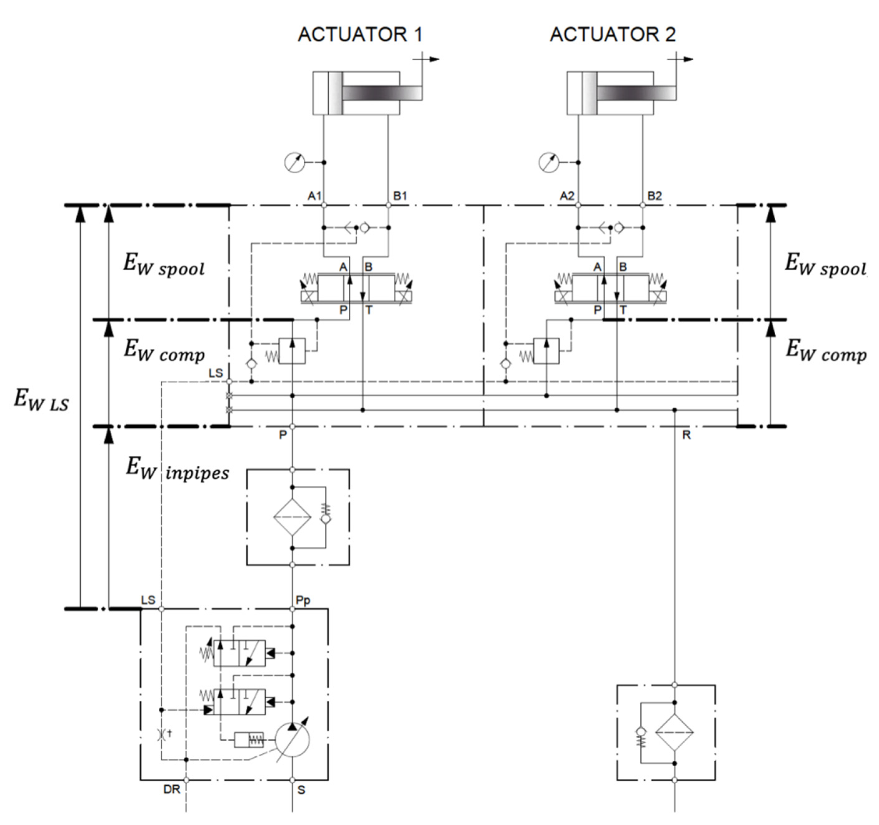
The system architecture is based on an Eaton 620 variable displacement piston pump with load-sensing pressure compensator and an Eaton CLS proportional sectional valve with pre-compensation. Overrunning loads, when present, are balanced with overcenter valves. Figure 2 shows the circuit being studied.

For this study, both instantaneous power and energy during a machine cycle have been considered. Both magnitudes have been calculated from the measured values.

Directly measured and calculated values are shown in Figure 3. The hydraulic power of the pump was calculated from the measured pressure and flow rate. The useful power in the actuators was obtained from the measured pressures and the flow rate calculated from the actuator speed. The wasted throttling power at the various restrictions was obtained from the measured pressures and the measured/calculated flow rates.

Sensors and their main characteristics are listed in

Table 2. Sensors and its characteristics.

Magnitude	Model	Range	Accuracy
Pressure	Wika OT-1	0–400 bar	0.5% span
Flow	Hydac EVS-3100-A-0300	0–300 L/min	2% act val.
Temperature	Ifm TA-2445	−50/+150 °C	0.3 °C
Position (extension)	Pepperl+Fuchs UB2000-F42-I-V15	90–2000 mm	1% act val.
Position (lift)	Waycon SX80-2500-1R-SA	0–2500 mm	2.5 mm
Position (catchers)	Hydac HLT-1100-R2L15C01-0450	0–450 mm	0.1 mm
Angle (tilt)	Pewatron G-NSDOG1-006-180	+/−180°	0.2°

. Calibration values were obtained from the manufacturer’s information and from comparison with a standard when the manufacturer’s information was not available. All values were checked in preliminary tests.

Sensor values were measured and recorded at a frequency of 1 kHz. Higher rates were not considered necessary for the energy analysis.

Digital filtering at 100 Hz was required for the calculation of the speeds, especially with the angle sensor. The data were processed with commercial software (DIAdem, Excel) to calculate the total energy consumption and identify where the energy is dissipated.

The tests were performed with different load conditions, from 100 kg to 500 kg. Special attention was paid to 100 kg, the most frequent loading condition according to the machine manufacturer’s information.

Figure 4 illustrates the three types of actuator considered in this study. The tilt actuator is double-acting rotary helical type, the lift actuator is a single-acting linear cylinder, and the extension and arm actuators are double-acting linear cylinders. This covers almost all types of actuators that can be found in typical mobile machinery.

The speed of each linear actuator ${\stackrel{·}{x}}_i$ is calculated from the measured position $x_i$, while the rotary actuator speed ${\stackrel{·}{\varphi }}_i$ is derived from the measured angle ${\varphi }_i$:

$${\stackrel{·}{x}}_i=\frac{\delta x_i}{\delta t}$$

(1)

$${\stackrel{·}{\varphi }}_i=\frac{\delta {\varphi }_i}{\delta t}$$

(2)

Flows across both sides of each linear actuator are calculated as follows:

$$Q_{Ai}={\stackrel{·}{x}}_i{S}_{Ai}$$

(3)

$$Q_{Bi}={\stackrel{·}{x}}_i{S}_{Bi}$$

(4)

Flow across the rotary actuator can be calculated as shown in Equation (5), where $K_{Fi}$ is the volumetric displacement of the actuator:

$$Q_i={\stackrel{·}{\varphi }}_i{K}_{Fi}$$

(5)

Linear actuator force is approximated from the measured pressures and the cylinder sections. This force includes the force to overcome the resistive friction forces and the force to accelerate the load.

$$\begin{array}{cc}Fi=& p_A{S}_A-p_B{S}_B\hspace{1em}(\mathit{Double} \mathit{acting} \mathit{cylinder})\\ & F_i=p_A{S}_R\hspace{1em}(\mathit{Single} \mathit{acting} \mathit{cylinder})\end{array}$$

(6)

Rotary actuator torque is approximated from the measured pressures and the specific torque $K_{Ti}$:

$$T_i=\left(p_A-p_B\right)K_{Ti}$$

(7)

The hydraulic power and energy of every actuator are giving as follows:

$$N_{ACT.i}=F_i{\stackrel{·}{x}}_i=T_i{\stackrel{·}{\varphi }}_i$$

(8)

$$E_{ACT.i}={\int }_0^t{N}_{ACT.i}dt$$

(9)

Energy is dissipated in the different parts of the circuit. Any fluid flow through a valve, pipe, hose or fitting requires a certain pressure difference $\mathsf{\Delta }p=P_{IN}-P_{OUT}$. Consequently, some of the incoming hydraulic power is wasted and dissipated as heat. The throttling wasted power $N_{W.i}$ and energy $E_{W.i}$ are calculated from the measured differential pressures and the calculated flow rates according to the following equation:

$$N_{W.i}=\mathsf{\Delta }{p}_i{Q}_i$$

(10)

$$E_{W.i}={\int }_0^t{N}_{W.i}dt$$

(11)

Energy losses can be calculated on a point-by-point basis. Figure 5 illustrates an example for the tilt actuator rotating forwards.

In a first approximation, the system losses can be calculated point to point and grouped into $E_{W inletpipes}$ (losses in pipes and accessories between the pump outlet and the inlet of the proportional valve), $E_{W Vsupply}$ (proportional valve throttling losses in the pressure compensator and in the flow supply path of the spool), $E_{W actpipes}$ (pipes and accessories losses in A and B port lines of the proportional valve), $E_{W Lctrl}$ (losses in valves for the control of overrunning loads), $E_{W Vreturn}$ (losses in the return flow path of the proportional valve spool) and $E_{W outletpipes}$ (losses in pipes and accessories between the proportional valve outlet and the tank).

Similarly, the overall losses in pipes and accessories are grouped as follows:

$$E_{W pipes}=E_{W inletpipes}+E_{W actpipes}+E_{W outletpipes}$$

(12)

For each actuator, hydraulic losses can be expressed as the sum of:

$$E_{Wi}=E_{W pipes}+E_{W Vsupply}+E_{W Lctrl}+E_{W Vreturn}$$

(13)

The hydraulic efficiency of a hydraulic system ${\eta }_{HYD}$ can be defined as the ratio between the energy delivered to the actuators ${\displaystyle \sum }_{i=1}^n{E}_{ACT,i}$ and the energy supplied by the hydraulic pump $E_{PUMP}$:

$${\eta }_{HYD}=\frac{{{\displaystyle \sum }}_{i=1}^n{E}_{ACT,i}}{E_{PUMP}}$$

(14)

The energy delivered to each actuator $E_{ACT,i}$ encompasses the energy that performs the useful work, $E_{useful,i}$, and the energies to lift and accelerate the structure $E_{pot,i}$ and $E_{kin,i },$ which are usually dissipated as heat throughout the machine cycle, but can actually be recovered and reused.

$$E_{ACT,i}=E_{useful,i}+E_{pot,i}+E_{kin,i}$$

(15)

Using Equation (16), the energy to lift a mass $m$ by a distance ${\mathsf{\Delta }}_h$ through a gravitational field of force $g$, can be calculated as:

$$E_{pot}=mg{\mathsf{\Delta }}_h$$

(16)

The kinetic energy of a body with mass $m$ and linear motion at speed $\stackrel{·}{x}$, or a body with rotational inertia $J$ rotating at speed $\stackrel{·}{\varphi }$, can be expressed as follows:

$$E_{kin}=\frac{1}{2}m{\stackrel{·}{x}}^2=\frac{1}{2}J{\stackrel{·}{\varphi }}^2$$

(17)

Considering the energies that can be recovered and reused, the net hydraulic efficiency ${\eta }_{HYD,net}$ can be defined as:

$${\eta }_{HYD,net}=\frac{{\sum }_{i=1}^n{E}_{ACT,i}-\left(E_{pot,i}+E_{kin,i}\right)}{E_{PUMP}}$$

(18)

3. Results

From test results and using the equations mentioned above, the hydraulic efficiency at different load conditions is calculated.

Table 3. Energy supplied, energy demanded and hydraulic efficiency for each load condition.

$\mathbf{Load} \left(\mathbf{k}\mathbf{g}\right)$	${\mathit{E}}_{\mathit{P}\mathit{U}\mathit{M}\mathit{P}} \left(\mathbf{k}\mathbf{J}\right)$	${\mathit{E}}_{\mathit{L}\mathit{I}\mathit{F}\mathit{T}} \left(\mathbf{kJ}\right)$	${\mathit{E}}_{\mathit{E}\mathit{X}\mathit{T}} \left(\mathbf{kJ}\right)$	${\mathit{E}}_{\mathit{T}\mathit{I}\mathit{L}\mathit{T}} \left(\mathbf{kJ}\right)$	${\mathit{E}}_{\mathit{L}\_\mathit{C}\mathit{A}\mathit{T}} \left(\mathbf{kJ}\right)$	${\mathit{E}}_{\mathit{R}\_\mathit{C}\mathit{A}\mathit{T}} \left(\mathbf{kJ}\right)$	$\mathbf{\sum }{\mathit{E}}_{\mathit{A}\mathit{C}\mathit{T}} (\mathbf{kJ})$	${\mathit{\eta }}_{\mathit{H}\mathit{Y}\mathit{D}}$
100	245.3	36.4	9.9	10.5	0.9	0.8	58.5	0.24
200	253.8	38.1	9.8	12.5	0.9	0.8	62.1	0.24
300	248.3	40.1	10.2	14.3	0.9	0.8	66.3	0.27
400	246.0	42.1	8.8	16.5	0.9	0.8	69.1	0.28
500	247.4	43.7	8.9	18.2	0.9	0.8	72.5	0.29

summarizes, for each load condition, the energy delivered by the pump, the sum of the energies delivered to the actuators (lift, extension, tilt and left and right container catchers) and the hydraulic system efficiency.

The resulting hydraulic efficiencies of between 0.24 and 0.29 are in the expected range for a LS system with a pump feeding several actuators in simultaneous operation. Another fact observed is that the load has little influence on the energy demand of the actuators. It deserves further analysis, but suggests that the self-weight of the structure is considerable. Similarly, although efficiency is higher with higher loads, as expected, the load has little influence on hydraulic efficiency. Figure 6 summarises the energy demand of the actuators.

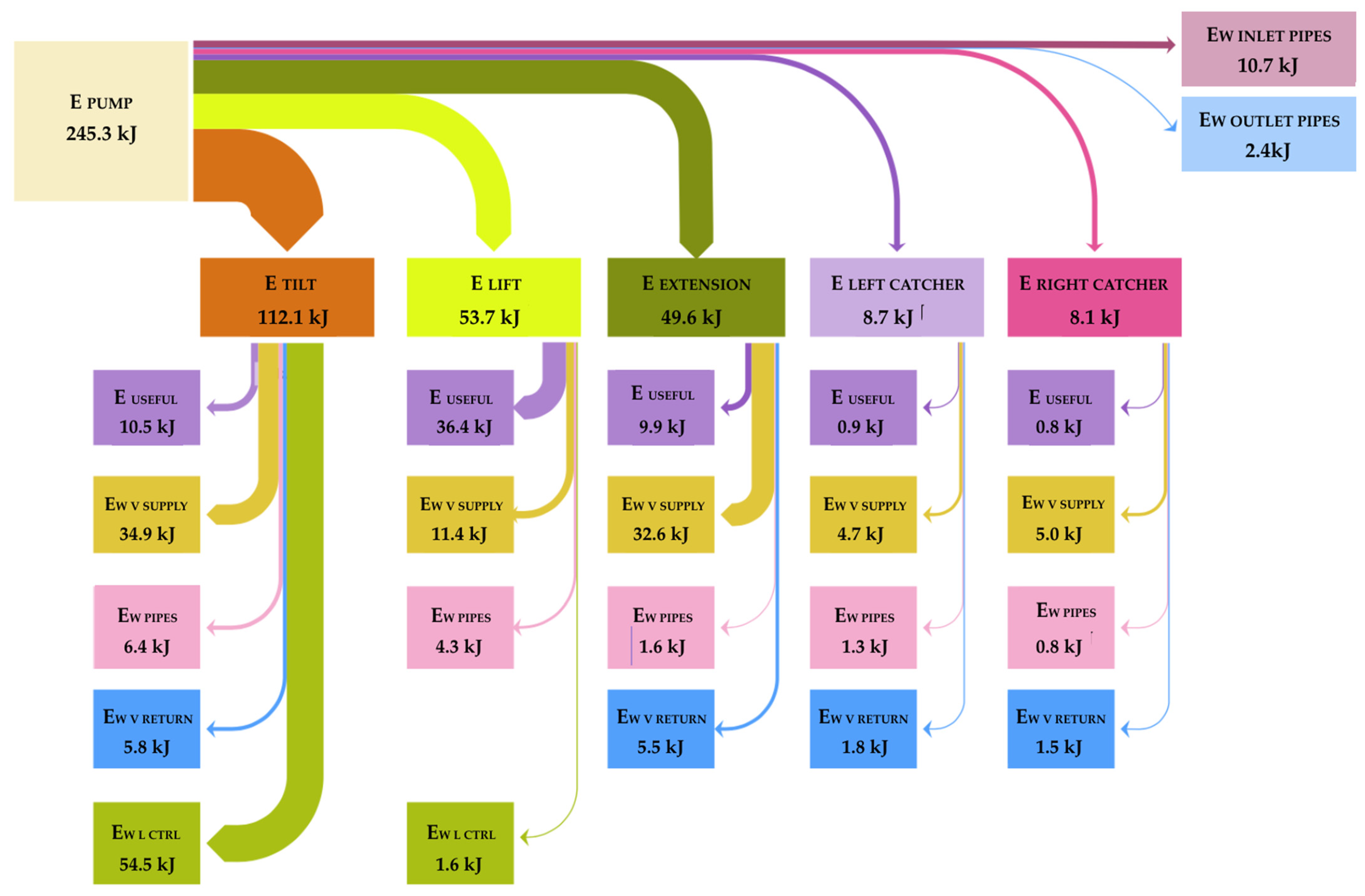
Figure 7 shows a Sankey plot of the hydraulic energy flow for a machine cycle with 100 kg load, the most frequent situation in real operation. The hydraulic energy demanded by each actuator and the hydraulic energy losses for each valve and pipe of the circuit have been calculated.

According to Figure 6 and Figure 7, the actuators with the highest energy demand (useful energy) are the tilt, lift and extension actuators, while the left and right catchers require a low percentage of the machine’s energy and do not deserve further analysis.

The Sankey plot gives valuable information on the energy flows of the system. It can be easily seen that the main energy losses are located in the supply paths of the proportional valve of the tilt and extension actuators and in the load control valves of the tilt actuator. Smaller, but also significant losses are due to the system piping and the supply path of the proportional valve of the lift actuator.

Especially significant is that the tilt actuator receives 112.1 kJ, the highest value of energy, the useful energy being only 10.5 kJ, a much lower value than the useful energy of the lift actuator (36.4 kJ), which receives 53.7 kJ. The energy received by the extension actuator (49.6 kJ) is also much higher than the useful value (9.9 kJ). Both tilt and extension actuators have low energy efficiency and deserve further analysis.

The total hydraulic losses of the system $\sum E_{Wi}$ are about 187 kJ and can be divided as shown in Figure 8. The main energy losses are located in the load control valves and in the proportional valve supply paths. The losses in the tilt, lift and extension actuators are plotted separately in Figure 9.

In both lift and extension actuators, throttling through the proportional valve supply path is the main source of losses, being associated with load sensing differential pressure and parallel operation of actuators with a pump.

The load control valve losses are small in the lift actuator because the valve is bypassed during lifting and the throttling losses are not taken into account when the assistive load is creating the motion. That is also the reason why $E_{WVreturn}$ is zero in the lift actuator. The extension actuator works horizontally and does not need valves for load control.

In the tilt actuator, the energy losses associated with the control of overrunning loads are considerable. While these results are useful, important questions about the efficiency improvement strategy remain open such as:

In the pressure valve supply losses, what is the percentage associated with parallel operation and what is the percentage associated with the LS pressure differential?

How much of the potential and kinetic energy can be recovered?

To answer these questions, a different approach is needed. A hydraulic system based on load sensing requires a minimum overpressure at the pump output with respect to the highest load pressure, to ensure the necessary oil flow through the proportional valve and guarantee sufficient dynamic response. Thus, the pump pressure is the highest load pressure of the actuators plus an additional constant pressure $\mathsf{\Delta }{p}_{LS}$.

The losses associated with the load sensing architecture for each actuator can be calculated as shown in Figure 10 and Equation (19):

$$E_{W LS,i}=E_{W inpipes,i}+E_{W comp,i}+E_{W spool,i}$$

(19)

Figure 11 shows a complete machine cycle indicating the sum of the power demanded from all actuator and differentiating 21 phases according to the actuators that are working simultaneously. The red line only takes into account the demanded power (resistive), i.e., the minimum power demanded from the pump in a system without power losses. The blue line, in which the assistive power is subtracted, clearly shows that there is a significant potential for energy recovery.

It is also observed that in nine phases there is more than one actuator working simultaneously. This causes energy losses in the system, as the pump must ensure the highest pressure from all actuators operating at the same time. The excess energy is dissipated in the pressure compensators of the less loaded sections.

Table 4. Energy dissipated as a result of the load-sensing pressure differential.

Actuator	${\mathit{E}}_{\mathit{W} \mathit{L}\mathit{S}\mathit{d}\mathit{i}\mathit{f}} \left(\mathbf{k}\mathbf{J}\right)$
Lift	20.6
Extension	9.5
Tilt	3.3
Catchers	10.9
$\sum$	44.3

and

Table 5. Energy dissipated in the less loaded actuators (phases with parallel actuation).

Phase	${\mathit{E}}_{\mathit{W} \mathit{p}\mathit{a}\mathit{r}\mathit{a}\mathit{l}\mathit{l}} \left(\mathbf{k}\mathbf{J}\right)$
2	0.7
3	9.1
4	6.5
11	0.8
14	22.8
16	1.1
18	0.5
19	2.6
20	0.2
$\sum$	44.3

summarise the energy dissipated due to load-sensing pressure differential $E_{W LSdif}$, and due to parallel operation, $E_{W parall}$, respectively.

Note that the sum of both losses coincides with the proportional valve supply path losses in the Sankey plot of Figure 5. According to the results, half of the losses are due to the pump load sensing pressure differential and the other half to the parallel operation of the actuators.

The analysis of quadrant operation is a very useful approach for energy study, since it takes into account the direction of the load with respect to the motion, which allows differentiation between resistive and assistive load conditions.

The force acting on the different actuators is due to both external forces and the weight of the machine structure. Depending on the direction of motion and force, each actuator experiences either a resistive force opposing its motion (quadrants I and III) or an assistive force assisting its motion (quadrants II and IV). In resistive quadrants I and III, the actuator must be supplied with power, with the design goal being to reduce the power supplied.

In assistive quadrants II and IV, the actuators can actually supply power to the system, but nevertheless, it is often necessary to supply additional power to control the positive loads. In this case, the goal is not only to reduce the power supplied to the actuator but also to use the actuator to supply power the system if possible. Figure 1 shows the load conditions of the different actuators.

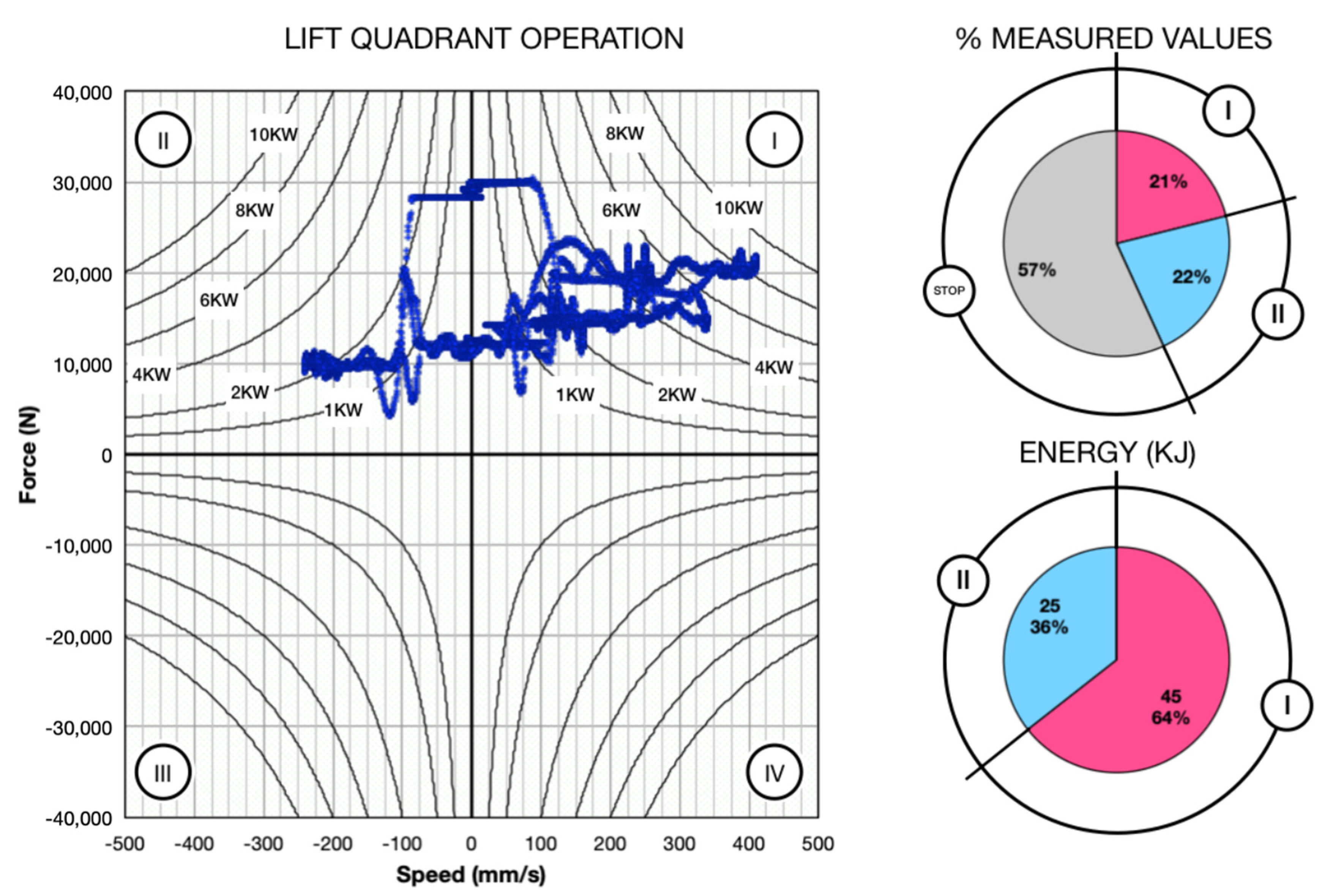
Figure 12 shows the analysis of the quadrant operation of the lift actuator based on the measured pairs of force and speed values. The left chart reveals that this actuator only operates in resistive quadrant I (lifting against the load) and in assistive quadrant II (lowering the load). According to the upper right pie chart, the actuator remains stopped for more than half of the cycle and when in motion, approximately 50% of the measured values are in quadrant I and the other 50% in quadrant II. As shown in the lower right pie chart, although the operating points are equally distributed between quadrants I and II, there is more energy in quadrant I than in quadrant II. The reason is that the container is lifted loaded, but lowered once unloaded. The power demand in quadrant I is high, reaching maximum values of 9 kW with an energy demand of 45 kJ.

Considering quadrant II as an opportunity to recover energy, there are 25 kJ that can potentially be reused, with power values up to 2.5 kW.

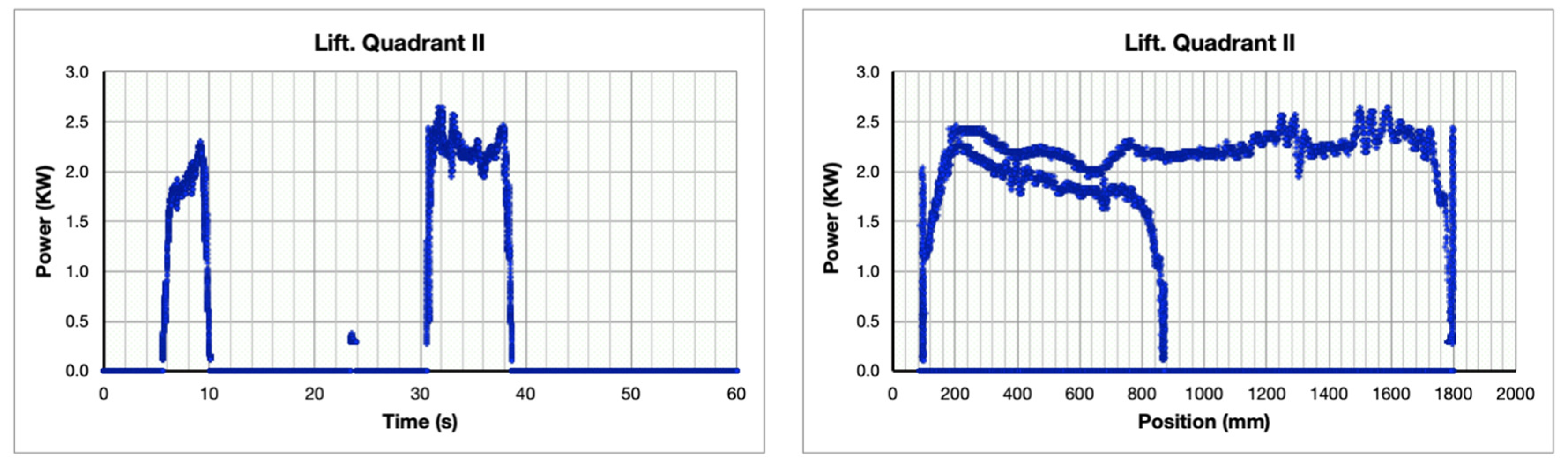
According to the results, the only quadrant in which the lift actuator recovers energy is II. Figure 13 shows the recoverable power as a function of time and position. In the chart of the left side it is possible to clearly differentiate the two periods of the machine cycle in which the lift actuator is lowering. In the chart of the right side it can be differentiated when the lift is lowering with and without load, showing that the load has little influence in the power demand. The shape of the curve in the charts clearly corresponds to a potential energy curve, being constant throughout the movement.

The results for the extension actuator are illustrated in Figure 14. This actuator operates in all four quadrants and is stationary 75% of the cycle. When in operation, most of the values are in resistive quadrants I and III, with maximum power values of 2 kW. The power demand is equally distributed, although it is slightly higher in quadrant III.

There are also some points measured in the assistive quadrant IV (4%), but always with power values below 1 kW and with an accumulated energy of 0.23 kJ, too low to be interesting to be recovered. The values in quadrant II are even lower and can also be discarded.

According to the Figure 14, the only quadrant to recover energy in the extension actuator is IV.

Figure 15 shows that the recoverable power is low. The shape of the curve in the chart of the right corresponds to a kinetic energy curve where the positions when the actuator is decelerating can be clearly seen.

Figure 16 shows the results for the tilt actuator, which also has four-quadrant operation. The actuator is stationary for almost 75% of the cycle. In operation, most of the values correspond to quadrants I and II, both with a similar number of operating points, but with almost double energy demand in quadrant I. As with the lift actuator, the reason is that the container is loaded most of the time in quadrant I, while in quadrant II it rotates without load. The recoverable energy in quadrant II is close to 3 kJ with power values up to 1 kW and there are some operating points in quadrants III and IV with lower energy values.

As shown in Figure 16, energy can be recovered from the tilt actuator in quadrants II and IV. The left charts in Figure 17 and Figure 18 show the states of the machine cycle when the tilt actuator is rotating with positive load, corresponding to quadrants II and IV. The curves in the right charts correspond to potential energy curves, varying with angle.

Table 6. Recoverable energy for each actuator in a cycle.

Actuator	Quadrant	${\mathit{E}}_{\mathit{R}\mathit{E}\mathit{C}} \left(\mathbf{k}\mathbf{J}\right)$	${\mathit{E}}_{\mathit{T}\mathit{Y}\mathit{P}\mathit{E}}$
Lift	II	25.00	Potential
Extension	IV	0.23	Kinetic
Tilt	II	2.85	Potential
Catchers	IV	0.49	Potential

summarises the recoverable energy in the actuators for a complete cycle. In the lift actuator there is an opportunity to recover energy, while the recoverable energy in the extension actuator and the catchers is too low. The tilt actuator deserves further analysis.

Figure 12, Figure 14 and Figure 16 provide a complete picture of the energy demand of the three main actuators, revealing the percentage of the machine cycle with each actuator in operation and allowing power and energy to be quantified. In addition, the recoverable energy can be easily quantified by looking at the values of the assistive quadrants II and IV.

However, the analysis of quadrant operation can give more interesting information. The pump pressure and flow rate can be compared to the effective pressure and flow rate of the actuators in each quadrant. In the resistive quadrants, the effective pressure is the value of pressure to move the load without backpressure in the opposite side of the actuator, while the effective flow rate is the flow rate supplied to the actuator. In the assistive quadrants, the effective pressure is the pressure to counterbalance the load without pressure in the supply side of the actuator and the effective flow is the exhaust flow from the actuator.

The effective pressure and flow rate for lift, extension and tilt actuators are calculated as shown in Appendix A.

Figure 19 summarises the information for analysing the lift actuator. The middle chart shows the pairs of effective pressures and flow rates for the pump (red) and the actuator (blue), including constant power hyperbolas to quantify the power of any operation point. The right and left charts show on the same scale the relative frequencies of the pressures and the bottom and top charts show the relative frequencies of the flows rates.

The central chart shows two pressure levels for quadrant I, one varying from 50 to 80 bar and the other constant at around 120 bar. The lower level corresponds to unloaded container movements with and the higher level to loaded container movements. The pump pressures are mostly slightly higher than those of the actuators, but there are also some points with much higher values, indicating the simultaneous movement of other actuators with higher load. As for the flow rates, the most common value for the pump is 60 L/min, while the most common values for the actuator are 10 and 30 L/min, which also coincides with parallel operation. The maximum power of the actuator is about 10 kW, while the pump reaches 20 kW.

In quadrant II, 80% of the pump pressure values are around 200 bar. The most frequent values of the actuator are 40 and 120 bar, both induced by the load. The hydraulic circuit of this actuator can be seen in Figure 2. When the load control valve is piloted for lowering, the maximum pump pressure is required through the load-sensing signal, which causes pump overpressure and consequent energy loss. The most frequent value of the flow is about 20 L/min (note that the actuator is simple acting and the flow during lowering is not supplied by the pump), while three different values can be observed for the pump: 5, 15 and 40 L/min.

Considering that quadrant II is assistive, so the actuator should not demand power from the pump, and that the pump is overpressurized due to the circuit architecture, leading to a power demand of up to 20 kW, there is a key point here to improve the efficiency of the system.

The results for the extension actuator are shown in Figure 20. The most frequent actuator pressure in the resistive quadrant I is around 20 bar, with values rarely exceeding 40 bar, while much higher pump pressures are observed, close to 40, 70 and especially 200 bar. Pump and actuator flow distributions are similar for values around 35 L/min, but pump values about 55 L/min also appear, indicating simultaneous parallel actuation of other actuators. As a result, pump power values in excess of 15 kW are observed, being considerably higher than power values required by the actuator, which do not exceed 2 kW. The results in quadrant III are similar, with actuator pressures below 40 bar and pump pressures of 80, 120 and 230 bar, pump flows above 60 L/min when actuator flow rates are below 30 L/min and pump power values of 20 kW with actuator demands of 2 kW. The data in quadrants II & IV are not relevant, indicating only parallel actuation in quadrant IV.

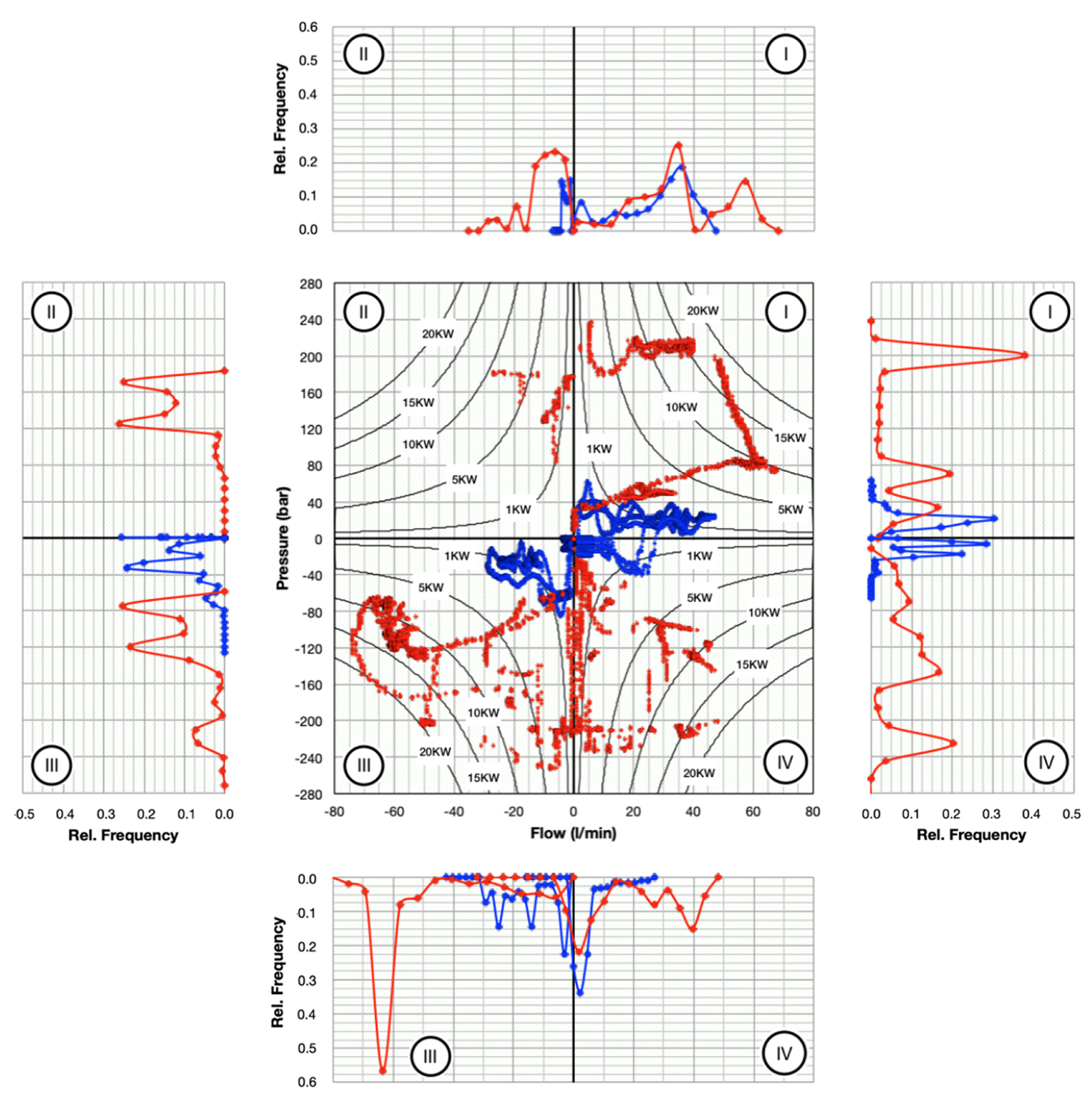
Figure 21 illustrates the tilt actuator data, where two concentric curves for the actuator pressures are observed. The outer curve corresponds to movements with loaded container and the inner curve to unloaded movements. The pump pressures in quadrant I have values around 120 and 200 bar, when the pressure required by the actuator does not reach 60 bar. The flow distributions do not differ much, with typical values of 35 and 60 L/min. Despite this, pump power reaches 20 kW while the actuator power is always below 5 kW, indicating that in this case the parallel actuation is not the main source of power loss. In quadrant III, typical pump pressures are 20, 80, 120 and 210 bar, with actuator pressures of 5, 20 and 50 bar. The pump flow distributions are quite similar, as in quadrant I, but pump power is again higher due to the pump overpressure.

In the assistive quadrants II & IV, the actuator and pump flow distributions are also similar, indicating that almost all of the pump flow goes to the actuator, i.e., minor parallel actuation. However, although the load should assist the actuator movement, pump pressure values of 60, 100 and 200 bar are observed in quadrant II, and 40, 140 and 220 bar in quadrant IV, which means that the load control valves are forcing the pump to deliver a large amount of power.

4. Discussion

This paper describes a multi-point-of-view analysis to identify the different sources of energy inefficiency in an existing hydraulic system. A mobile machine with load sensing architecture is studied, but other architectures or any industrial hydraulic application can also be the subject for a similar analysis.

The literature from which we have information only implements energy balances from a single point of view. The challenge is usually to deduct an approximate overall performance of the machine or to obtain an image of the energy balance. The results of this paper show that different approaches give complementary information to decide the right strategy to improve the hydraulic efficiency. With this methodology we are not only able to visualize the energy balance, estimate the total performance of the system and it’s potential for reducing energy consumption. More importantly, it shows at which points of the system there is excessive energy consumption and deduces the root of this high consumption. This information can be the starting point for optimizing the hydraulic system from an energetic point of view, allowing to choose more suitable, better-sized, better-controlled components, or, alternatively, to use innovative architectures.

A point-to-point calculation for different load conditions of the pump supplied energy and the demanded energy of each actuator gives overall results as hydraulic efficiencies between 0.24 and 0.29 and a low influence of the load in the hydraulic efficiency.

A point-to-point calculation of the energy losses and their representation through Sankey and circle plots shows the location of the losses (in this particular machine 55% of the losses are associated to the proportional valve, 30% to the load control valves and 15% to the pipes), but does not give enough information of the parallel operation losses and the potential for energy recovery.

Another interesting results of this first approach are:

-

The load has only little influence on the energy demand of the actuators, suggesting that the structure self-weight is considerable.

-

Load has only little influence on hydraulic efficiency.

-

Left and right catchers require a low percentage of the machine energy and do not deserve a deep analysis

Differentiating the cycle phases depending on the actuators working, identifying those with simultaneous operation and analysing them separately, helps divide losses due to parallel operation and load sensing differential (approximately 50% each concept in this case).

And last, the quadrant analysis for every actuator of useful and pump demanded power, showing the results in a 4-quadrant power map with constant power hyperbolas and including the relative frequencies of pressure and flow, results in a complete image of the system power that summarises rich information and allows to identify and quantify the recoverable energy. In this example, the results show that there is an important amount of potential energy to recover in the lift actuator (25 kJ) and some potential in the tilt actuator (2.85 kJ). In addition to this, a significant energy loss occurs during the lowering of the load with the lift actuator, which is produced when the load control valve is piloted for lowering. Then, maximum pump pressure is required through the load-sensing signal, causing pump overpressure and a consequent energy loss.

The results of this analysis indicate that the main sources of energy loss are those associated with parallel operation of actuators and control of overrunning loads.

Based on the results, there is room for improvement. The system architecture deserves a further analysis of the existing alternatives to minimise losses and attempt to recover the allowable potential energy. If the use of load control cannot be avoided, it is mandatory the use of energy-efficient models, setting them to the lowest values that guarantee the performance.

It is suggested that the next phase of the research should be to search for different solutions to improve the efficiency of the system, with special attention to alternatives to load control valves and system architecture, with independent metering being an interesting option.