Current-Based Bearing Fault Diagnosis Using Deep Learning Algorithms

Abstract

Artificial intelligence algorithms and vibration signature monitoring are recurrent approaches to perform early bearing damage identification in induction motors. This approach is unfeasible in most industrial applications because these machines are unable to perform their nominal functions under damaged conditions. In addition, many machines are installed at inaccessible sites or their housing prevents the setting of new sensors. Otherwise, current signature monitoring is available in most industrial machines because the devices that control, supply and protect these systems use the stator current. Another significant advantage is that the stator phases lose symmetry in bearing damaged conditions and, therefore, are multiple independent sources. Thus, this paper introduces a new approach based on fractional wavelet denoising and a deep learning algorithm to perform a bearing damage diagnosis from stator currents. Several convolutional neural networks extract features from multiple sources to perform supervised learning. An information fusion (IF) algorithm then creates a new feature set and performs the classification. Furthermore, this paper introduces a new method to achieve positive unlabeled learning. The flattened layer of several feature maps inputs the fuzzy c-means algorithm to perform a novelty detection instead of clusterization in a dynamic IF context. Experimental and on-site tests are reported with promising results.

1. Introduction

Induction motors are present in most industrial processes because of their versatility for many applications, efficiency and robustness to operate in severe conditions. Recent studies have reported that 40% of operational failures caused in these machines are related to damage from bearings, which can be separated into two categories. The first category is the punctual damages that appear on a delimited bearing surface producing an impulsive mechanical vibration. The second category is the distributed damages that produce continuous mechanical vibrations with low magnitude harmonics [1,2].

The most recurrent approach to achieving bearing condition monitoring and damage diagnosis is to acquire vibration-based signals from accelerometers and perform supervised learning algorithms. However, many industrial motors are unable to provide vibration signals because they are installed at inaccessible locations or their housings are inadequate to install new devices. The vibration data acquisition is also expensive, demanding new sensors and devices to transduce, transmit and process [3]. Otherwise, current-based data acquisition is available in most industrial electric motors because the stator current is monitored for control, supply and protection purposes. Consequently, each motor phase is a distinct data source for the machine status because the phases lose symmetry due to disturbances, interferences, noises, intrinsic conditions, bearing damage or other reasons [4,5].

In this context, the wavelet transform (WT) becomes a recurrent tool for signal processing because of its advantage of a multiresolution analysis. The fractional wavelet transforms (FWTs) generalize the WT to represent signals in the fractional time-fractional frequency domain, preserving sparsity, removing redundancy, denoising and narrowing the resolution [6,7]. Therefore, appropriate denoising and reconstruction proceedings can generate a database with multiple data sources from each motor phase.

Consequently, deep learning (DL) algorithms with a data-driven approach can extract abstract features from multiple sources to improve the classification task [8,9]. Autoencoders [10], variational autoencoders [11], convolutional neural networks (CNN) [12,13], generative models [14], recurrent neural networks (RNN) [15] and extreme learning [16], among others, construct feature maps with deep levels of data abstraction. Moreover, the DL approaches can outperform traditional signal processing techniques and feature extraction methods to perform a bearing damage diagnosis [8,17].

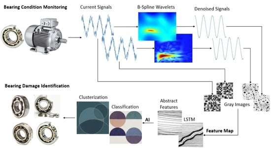
Thus, this paper introduces a new deep learning approach based on an FWT, an independent CNN and long short-term memory (LSTM) to perform bearing damage identification from multiple sources. The raw and denoised signals become the multiple inputs of the maps of several features with different receptive fields. Each feature map inputs an independent flattened layer (FL) that feeds several artificial neural networks (ANN) to perform supervised learning and a SoftMax classification. LSTM cells are introduced in the feature maps with a large receptive field to improve the long time-dependency feature extraction. An information fusion (IF) algorithm unifies each SoftMax output into a novel feature set, reducing multiple source redundancy and preserving the bearing condition monitoring. With this new approach, the information fusion problem is replaced by a supervised classification task performed by a support vector machine (SVM).

Otherwise, in most industrial applications, the electric motors with damaged bearings are prevented from performing their nominal functions because of industrial process safety reasons. The bearing damage produces vibration signatures that propagate to pumps, compressors, pipelines or other types of loads that affect processes or subsystems [18]. Therefore, the acquisition of a labelled database with several damages is unrealistic or impracticable for most industrial facilities. However, one-class positive unlabeled learning (PUL) algorithms can detect novelty in unlabeled databases. The positive class, in this case, is the healthy bearing signals [19,20].

Thus, this paper introduces a second new approach that uses the feature maps from multiple phases (raw and denoised sources) to input several fuzzy c-means (FCM) algorithms in a paradigm to detect novelty in PUL instead of clustering data. Assuming that a healthy class is available and two clusters are present in each source, the Fisher discriminant ratio (FDR) and the Kullback–Leibler divergence (KLD) can monitoring the center and distribution behavior. A similar IF approach unifies the FDR and KLD of each FCM into a new feature set, preserving the bearing condition monitoring while inputting a SoftMax classifier to perform the bearing damage identification. The results of experimental and on-site tests with both approaches (supervised and PUL) are promising.

The sequence of this paper presents the theoretical background in Section 2. The test rig, setup and configurations are described in Section 3. Section 4 describes experimental and on-site tests. Section 5 presents the conclusion.

2. Theoretical Background

2.1. Fractional B-Spline Wavelet Transform

Fractional B-splines (FS) are the extended version of splines with order α > −1 defined as:

$${\beta }_{\pm }^{\alpha }\left(x\right)=\frac{1}{\mathsf{\Gamma }\left(\alpha +1\right)}{\mathsf{\Delta }}_{\pm }^{\alpha +1}{x}_{\pm }^{\alpha }$$

(1)

where $k \in \mathbb{Z}$and $\mathsf{\Gamma }\left(\alpha +1\right)$ is the gamma function. The one-side causal function (+) is $x_{+}^{\alpha }=x^{\alpha }$ and the anti-causal (–) is $x_{-}^{\alpha }={\left(-x\right)}_{+}^{\alpha }$. The fractional finite difference operator is:

$${\mathsf{\Delta }}_{\pm }^{\alpha }f\left(x\right)={{\displaystyle \sum }}_{k=0}^{\infty }{\left(-1\right)}^k\left(\begin{array}{c}\alpha \\ k\end{array}\right)f\left(x\mp k\right).$$

(2)

The FS is obtained by interpolating polynomial B-splines. The centered fractional B-splines of degree α are defined by the convolution operator $\star$ as:

$${\beta }_{\star }^{\alpha }\left(x\right)={\beta }_{+}^{\frac{\alpha -1}{2}} \star {\beta }_{-}^{\frac{\alpha -1}{2}}$$

(3)

and ${\mathsf{\Delta }}_{*}^{\alpha }\leftrightarrow |1-e^{-jw}{|}^{\alpha }$ denotes the symmetric fractional finite difference operator. The Fourier transform of the one-side causal and centered fractional splines are calculated as follows:

$${\widehat{\beta }}_{+}^{\alpha }\left(w\right)={\left(\frac{1-e^{-jw}}{jw}\right)}^{\alpha +1}{\widehat{\beta }}_{\star }^{\alpha }\left(w\right)={\left(\frac{\sin \left(w/2\right)}{w/2}\right)}^{\alpha +1}.$$

(4)

Fractional B-splines satisfy all requirements to construct a wavelet basis for an α > −0.5 given by:

$${\beta }^{\alpha }\left(x/2\right)={\displaystyle \sum }_{k\in \mathbb{Z}}^{}{h}^{\alpha }\left(k\right){\beta }^{\alpha }\left(x-k\right)$$

(5)

where the filters $h_{+}^{\alpha }\left(k\right)$, $h_{-}^{\alpha }\left(k\right)$ and $h_{\star }^{\alpha }\left(k\right)$ are defined as:

$$\begin{array}{c}{h}_{+}^{\alpha }\left(k\right)=\frac{1}{2^{\alpha }}\left(\begin{array}{c}\alpha +1\\ k\end{array}\right)\leftrightarrow {\widehat{h}}_{+}^{\alpha }\left(w\right)=2{\left(\frac{1+e^{-jw}}{2}\right)}^{\alpha +1}\\ h_{\star }^{\alpha }\left(k\right)=\frac{1}{2^{\alpha }}\left(\begin{array}{c}\alpha +1\\ k\end{array}\right)\leftrightarrow {\widehat{h}}_{\star }^{\alpha }\left(w\right)=2{\left(\frac{1+e^{-jw}}{2}\right)}^{\alpha +1}.\end{array}$$

The anti-causal (–) is obtained by substituting $h_{-}^{\alpha }\left(k\right)=h_{+}^{\alpha }\left(-k\right)$. The general approach to orthonormalize the fractional splines generates the scaling function given by:

$$\varphi \left(x\right)={\displaystyle \sum }_{k\in \mathbb{Z}}^{}{\left(a_{\phi }^{\alpha }\left(k\right)\right)}^{-\frac{1}{2}}{\beta }^{\alpha }\left(x-k\right)$$

(6)

where ${(a_{\phi }^{\alpha }\left(k\right))}^{-1/2}$ is the convolution of the FS sequence. The Fourier transform $A_{\phi }^{\alpha }\left(w\right)$ is defined as:

$$a_{\phi }^{\alpha }={\beta }_{*}^{2\alpha +1}\left(k\right)A_{\phi }^{\alpha }\left(w\right)={{\displaystyle \sum }}_{k\in \mathbb{Z}}{\beta }_{*}^{2\alpha +1}\left(n\right)e^{-jwn}.$$

Leading the corresponding two-relation:

$$\varphi \left(x/2\right)={{\displaystyle \sum }}_{k\in \mathbb{Z}}{h}_{\perp }^{\alpha }\left(k\right)\varphi \left(x-k\right).$$

The low-pass filter and high-pass filter can be written as:

$$H_{\perp }^{\alpha }\left(w\right)={\widehat{h}}^{\alpha }\left(w\right)\sqrt{\frac{A_{\phi }^{\alpha }\left(w\right)}{A_{\phi }^{\alpha }\left(2w\right)}}{G}_{\perp }^{\alpha }\left(w\right)=e^{-jw}\overline{H_{\perp }^{\alpha }\left(w+\pi \right)}.$$

Thereby, the behavior of the filter tends to an ideal low-pass and high-pass filter as $\alpha \to 0$ [6,21]. The overlapping group shrinkage (OGS) algorithm reconstructs the denoised signal by observing the wavelet coefficients and performing a convex regularization while minimizing a cost function [22,23]. Therefore, in this paper, the equivalent filter bank denoises the raw signals to input the feature maps.

2.2. Long Short-Term Memory

A recurrent neural network (RNN) is a class of ANN that identifies patterns in sequential data. However, an RNN has a few drawbacks for most applications including gradient vanishing and gradient explosion in the backpropagation. Long short-term memory (LSTM) solves the gradient vanishing problem, using a memory cell that improves the RNN units [24,25]. Figure 1 shows a typical LSTM cell.

The LSTM gates control the information flow of the current state, the input gate (i) and the output gate (o) [25]. The forget gate (f_t) determines how much previous information should be removed or saved as follows:

$$f_t=\sigma \left(w_{fz}{z}_t+w_{hf}{h}_{\left(t-1\right)}+b_f\right)$$

where $\sigma$ is a sigmoid function, $w$ is the weight, $z_t$ is the current input, $h_{\left(t-1\right)}^{}$ is the output of the previous cell and $b_f$ is the bias. The input gate determines the behavior of $x_t$, the previous layer $h_{\left(t-1\right)}$ and the current state ($Ct$) as follows:

$$\begin{array}{c}{i}_t=\sigma \left(w_{zi}{z}_t+w_{hi}{h}_{\left(t-1\right)}+b_i\right)\\ {\widehat{C}}_t=\tan \mathrm{h}\left(w_{xc}{z}_t+w_{hc}{h}_{\left(t-1\right)}+b_i\right).\end{array}$$

The output gate controls the cell information and state as follows:

$$\begin{array}{c}{c}_t=c_{t-1}{f}_t+i_t{\widehat{C}}_t\\ o_t=\sigma \left(w_{zo}{z}_t+w_{ho}{h}_{\left(t-1\right)}+b_o\right)\\ h_t=o_t\times \tan \left(c_t\right).\end{array}$$

Thus, the LSTM can memorize relevant time-dependent features to discriminate long-time delay events with overlapping low-frequency components [26].

2.3. Convolutional Neural Networks

The basic CNN contains three structures that provide feature extraction, perform classification and represent the decision with a probabilistic function. The convolution layer (CL) performs dot products, preserving the spatial structure of the previous layer and output abstract features [27,28]. The convolutional process is described as follows:

$$x_j^l=f\left({\displaystyle \sum }_{i \in M_j}{x}_i^{l-1}\ast k_j^l+b_j^l\right)$$

(7)

where $\ast$ is the convolution operation and $x^{l-1}$ denotes the input data of the previous layer. Each layer consists of $n^l$ kernels with a weight matrix $k_j^l$ and a bias vector $b_j^l$. The output of the nonlinear active function $f(\ast )$ is the $n^l$ matrices $x_j^l$ where $j=1 : n^l$ corresponds with $n$ kernels from the layer $l$. The activation function leaky-Relu has a linear identity for positive values and a slope for negative values to avoid gradient problems.

The pooling layer (PL) down-samples the previous CL to control the feature map size and save abstract information. The function $\max \left(x_j^l\right)=x_j^{l+1}$ is the most recurrent down-sampling operation in CNN models. Therefore, the feature map is an independent structure containing successive CLs and PLs that control the size and depth to extract more abstract features. The last PL can input LSTM cells to extract time-dependent features or be transformed into a flattened layer (FL) to input an ANN or other classifier [27,28]. The third structure is the SoftMax probabilistic distribution operator that transforms the classifier output $z_i$ into a normalized vector as follows:

$$p_i=\frac{e^{\left(z_i\right)}}{{{\displaystyle \sum }}_{j=1}^N{e}^{\left(z_j\right)}}{p}_i\in \left[0,1\right].$$

(8)

These three structures are used in different configurations to extract abstract features and improve accuracy classification. The feature maps can also be arranged in parallel with profound and shallow receptive fields to extract features from multiple sources [29].

2.4. Fuzzy C-Means Algorithm

The one-dimensional FL with data $X=\left\{x_1, x_2, \dots x_k\right\}$ inputs the FCM algorithm to divide $X$ into several clusters. The objective function of the FCM is defined as follows:

$$\begin{array}{c}J={\displaystyle \sum }_{i=1}^c{\displaystyle \sum }_{j=1}^k{u}_{i,j}^m{\left|\left|x_j-v_i\right|\right|}^2\\ s.t.{\displaystyle \sum }_{i=1}^c{u}_{ij}=1,0\le u_{ij}\le 1\end{array}$$

where $U={[u_{ij}]}_{c\times k}$ is a membership matrix, $m>1$ is the fuzzifier, $v_i$ are the prototypes and c is the number of clusters. The solution for updating the partition matrix and the prototypes is given by:

$$u_{i,j}=\frac{{({\left|\left|x_j-v_i\right|\right|}^2)}^{-\frac{1}{m-1}}}{{{\displaystyle \sum }}_{q=1}^c{({\left|\left|x_j-v_q\right|\right|}^2)}^{-\frac{1}{m-1}}}{v}_i=\frac{{{\displaystyle \sum }}_{j=1}^k{u}_{i,j}^m{x}_j}{{{\displaystyle \sum }}_{j=1}^k{u}_{i,j}^m}.$$

A recurrent approach to stop criteria is a threshold between two successive partitions [30]. The fuzzy C-means can perform bearing detection and classification in an unlabeled context, presenting remarkable results with vibration-based signals. The main advantage is that the FCM algorithm allows changes in the regularization, cluster shape, cost function and membership function to improve the performance. The intra-cluster variance can also be minimized by adjusts in the fuzzifiers, keeping an adequate boundary. Indeed, the support vector data description (SVDD) and the one-class SVM present boundary problems including loose boundaries, data rejection and outlier misclassification among others that increase the complexity of the distribution interpretation and classification.

In this paper, the Fisher discriminant ratio (FDR) and Kullback–Leibler divergence (KLD) perform center monitoring and distribution behavior in the PUL context. Initially, an FL from a healthy source inputs the FCM algorithm, configurated in a paradigm to identify two clusters. Therefore, if the input remains healthy, the difference between the centers and distribution divergence must remain constant after successive batches.

2.5. Information Fusion

Multiple sources can merge into a new feature set throughout information fusion algorithms (IF) [31,32]. Assuming that $s$ samples, $c$ classes and $n$ independent sources and classifiers are available, the features set from each source $X^n$ is represented as follows:

$$\begin{array}{c}{X}^1=\left[x_1^1,x_2^1,\dots ,x_s^1\right]\\ X^2=\left[x_1^2,x_2^2,\dots ,x_s^2\right]\\ X^n=\left[x_1^n,x_2^n,\dots ,x_s^n\right].\end{array}$$

Therefore, n feature sets input n CNNs to classify $C_i$ classes in each feature set $X^n$. The conditional probability $P(\cdot |\cdot ,\cdot )$ of the class i based on the observation of k CNN on the sample $x_j^k$ is defined as:

$$P_i^{k,j}=P\left(C_i|x_j^k,CN{N}^k\right)i=1:cj=1:sk=1:n.$$

(9)

All combinations of $CN{N}^k$ are rearranged in the matrix $P^k$ with the size $c\times s$. The output of all classifiers is then merged to the $\left(c\times n\right)\times s$ matrix P as follows:

$$P_{}^k=\left[\begin{array}{ccc}{P}_1^{k,1}& \cdots & P_1^{k,s}\\ ⋮& \ddots & ⋮\\ P_m^{k,1}& \cdots & P_m^{k,s}\end{array}\right]P=\left[\begin{array}{c}{P}^1\\ ⋮\\ P^n\end{array}\right].$$

(10)

The task of analyzing multiple sources becomes a task of classifying the new feature set P. Consequently, the IF approach for the FCM is similar. The flattened vector from n feature maps input n FCM. The s samples are replaced by batches with measures $m_j^{}$ (KLD and FDR) to form the feature sets:

$$\begin{array}{c}{X}^1=\left[FD{R}_1^1,KL{D}_1^1, \dots ,FD{R}_s^1,KL{D}_s^1\right]\\ X^2=\left[FD{R}_1^2,KL{D}_1^2,\dots ,FD{R}_1^2,KL{D}_1^2\right]\\ X^n=\left[FD{R}_1^n,KL{D}_1^n,\dots ,FD{R}_1^n,KL{D}_1^n\right].\end{array}$$

Therefore, n FCM identifies the healthy class $\left(c=1\right)$ or detects the novelty $\left(c=2\right)$ of $X^n.$ The conditional probability $P(\cdot |\cdot )$ of the class $C_i$ based on the observation of k FCM on the measure $m_j^k$ is defined as:

$$P_i^{k,j}=P\left(C_i|m_j^k,FC{M}^k\right)i=1:cj=1:sk=1:\mathrm{n}.$$

(11)

This new approach leads to similar $P^k$ and P matrices of Equation (10), which depends on the FCM performance, batch size and number measures.

3. Datasets

The tests were performed with every current-based signal developed by the Chair of Design and Drive Technology from the University of Paderborn in Germany containing the current-based signals from an induction motor. Two current probes acquired signals from the test rig with a sampling frequency of 64 kHz, a rotor speed of 900 rpm and 1500 rpm (N09 and N15) and loading conditions of 0.1 Nm and 0.7 Nm (M01 and M07). The classes of these damages were healthy and incipient, distributed and punctual damages [33]. In this test rig, the bearings were located externally from the induction motor to extract more sensitive vibration-based information. However, the internal bearings produced a few effects in data distribution that might cause misclassification in machine learning algorithms that learn from external bearing damage.

This work also used the test rig available at CISE, Electromechatronic Systems Research Centre at the University of Beira Interior in Portugal, to acquire bearing damaged current-based signals. The test rig consisted of an inverter-fed three-phase squirrel-cage induction motor, a programmable AC power source of 0~300 V, 12 kVA, 192 Amps, 15~1.2 kHz (Chroma), a data acquisition device USB-6366 (National Instruments) and a mechanical system that provided a stable load with speed control. Two current probes sent the stator currents to the acquisition board with a sampling frequency of 44 kHz, producing samples with a rotor speed of 1800 rpm and loading conditions of 0.1 Nm and 0.7 Nm. The first CISE damaged bearing had an incipient punctual damage in both rings caused by electrical discharges. The inner ring damage diameter was 1.5 mm and the spheres and cage remained intact. The outer ring had two opposite damages with diameters of 2.0 mm and 1.5 mm. This type of damage is common in industrial machinery but it was absent in the Padeborn dataset. The second CISE damaged bearing had punctual damage (hole) of 2.0 mm in the outer ring. Different from the Padeborn test rig, the CISE test rig inserted the damaged bearing at the fan on the drive-end side of the induction motor.

Pre-Processing

All stator phases (R1 and R2) of each bearing damage from both datasets were denoised with a FWT and reconstructed with the OGS algorithm to generate F1 and F2 signals. Several signal segments were then rearranged in a square matrix $t\times t$ to convert 1-D signals into grayscale images (base2). In this work, the segment $t$ was defined by the lower motor speed that produced (64,000$\times$ 60)/900 samples per revolution ($\simeq$4266). Therefore, $t^2=4096$ samples produced the normalized gray images with a size of 64 $\times$ 64. The sets of gray images from R1, R2, F1 and F2 sources inputted two independent arranges (A1 and A2) of feature maps with a profound and shallow receptive field.

Table 1. Feature map architecture with a profound receptive field (A1).

Layer	K. Size	K. Number	Input	Output
CL 1	9 × 9	4	64 × 64	64 × 64
PL 1	2 × 2	4	64 × 64	32 × 32
CL 2	7 × 7	6	32 × 32	32 × 32
PL 2	2 × 2	6	32 × 32	16 × 16
CL 3	5 × 5	8	16 × 16	16 × 16
PL 3	2 × 2	8	16 × 16	8 × 8
CL 4	3 × 3	10	8 × 8	8 × 8
PL 4	2 × 2	10	8 × 8	4 × 4
FL			10 × 16	1 × 160

summarizes the profound configuration, which was a conventional feature map with four CLs and PLs.

The feature map with a profound receptive field (A1) consisted of successive CLs and PLs to extract deeper abstract features. The kernel size of the CLs reduced, concentrating the abstract information into more compact structures, increasing the number of kernels. This procedure allowed the extraction of more abstract features with different kernel configurations. The PL controlled the output size through down-sampling operations while grouping relevant information, allowing the CL to increase the kernel number. The last PL inputted an FL with a 1 × 160 dimension. Thus, this feature map was capable of extracting abstract information at each CL, increasing the number of kernels to diversify the feature type.

The shallow receptive field (A2) was a feature map with two successive CLs and PLs and LSTM cells to extract long time-dependent features. In this configuration, the last cell of LSTM 2 also inputted an FL.

Table 2. Feature map architecture with a shallow receptive field and LSTM cells (A2).

Layer	K. Size	K. Number	Input	Output
CL 1	9 × 9	5	64 × 64	64 × 64
PL 1	4 × 4	5	64 × 64	16 × 16
CL 2	7 × 7	10	16 × 16	16 × 16
PL 2	4 × 4	10	16 × 16	4 × 4
LSTM 1		32 cells	10 × 16	10 × 32
LSTM 2		16 cells	10 × 32	1 × 16

summarizes the shallow configuration.

This feature map consisted of a particular arrangement (A2) to extract shallow abstract features within a large receptive field. The CL and PL controlled the feature map size, avoiding deep features and allowing diversity in the kernels. The PLs reduced the feature map size, revealing inner relations in each kernel. PL 2 inputted the LSTM cells that behaved as recurrent neural networks, saving relevant time-dependent features to input an FL. Indeed, the main advantage of the LSTM cells was that the internal structures controlled the flow of relevant information, keeping long-time relevant features.

In summary, the multiple sources (4) inputted each feature map arrangement (2) to generate eight independent FLs. The supervised learning was performed by eight ANNs with a stochastic gradient descent, a learning rate at 0.0015, momentum at 0.5 and L2 regularization. The training set contained 1000 samples for each class (4000 in total) while the test set had 250 samples for each class. Each SoftMax had four outputs corresponding with each class. The IF unified the output from each SoftMax into the P matrix and a support vector machine performed the classification task. All possible four class combinations with different severity indexes were performed and the results were presented in terms of average accuracy.

Otherwise, in the PUL context, the objective was to identify incipient bearing damage using the KLD and FDR measures from FCM algorithms. Therefore, all possible combinations for healthy versus damaged signals with A1 and A2 arranges were performed.

4. Experimental and On-Site Tests

4.1. Supervised Learning

This research compared R1 and R2 and F1 and F2 performance to verify the effectiveness of the IF. The average accuracy of three operation conditions (N15M01, N09M07, N15M07) is summarized in

Table 3. Average accuracy of supervised learning.

Source	Earlier	Punctual	Distributed
R1	91.38	94.82	91.87
R2	90.26	94.76	91.74
F1	91.70	95.21	92.24
F2	91.92	96.43	92.18
R1 and R2	93.56	95.97	92.65
F1 and F2	93.82	96.65	93.32
IF	94.11	97.02	93.55

.

The performance of F1 and F2 reached a similar accuracy of the IF with the four signals. Considering the implementation aspect, one can choose to fuse the F1 and F2 sources instead of performing the four sources (IF) to reduce the computational efforts, keeping a high accuracy performance. However, all tests performed in this paper were conducted with four sources in an IF context. Condition N15M07 improved the accuracy for each type of damage while the other two conditions decreased the average. An SVM with a linear kernel and a soft margin approach performed the P matrix classification. The setup of hyperparameters, training, stop criteria and kernel configurations were omitted for the sake of brevity. The polynomial and Gaussian kernels performed similar results although with more convergence time.

4.2. Unlabeled Learning

Five recent FCM algorithms were performed to identify novelty in a one-class PU context. The first was the FCM with a genetic optimization (FCM-GO) algorithm that searched for a suboptimal solution [34]. The Gustafson–Kessel (GK) clustering algorithm employed the Mahalanobis distance to update centers and proto-clusters. The FN-DBSC could be characterized by a convex function with a particular set of hyperparameters [35]. The FCM with a focal point (FCMFP) introduced a regularization term into the loss function [35]. Lastly, the Gath-Geva (GG) clustering is an extended version of the FCM that performed the previous detection of sizes and densities of clusters [36]. These fuzzy-based algorithms could perform novelty detection in the PUL context with an appropriate initialization method.

Assuming that two clusters were present in the PU data distribution, a previous batch $\left(-\tau , t_0\right)$ defined the centers and boundaries of these pseudo-clusters. In parallel, the KLD and FDR measured the distribution and the center behavior. A successive batch with current data $(t_0,-\tau ,)$ was then used to calculate two new pseudo-clusters. The comparison between the KLD and FDR of previous and current batches identified the changes in the PU data. Figure 2 resumes the cluster behavior of the FCM algorithms in a one-class PU novelty detection paradigm.

Thus, the KLD and FDR measures could identify changes in the data distribution to perform novelty detection. In this case, a healthy bearing signal produced small changes in these measures because their outliers and noises were uncorrelated with bearing damage. Consequently, when damage arose, the previous cluster contained data from the healthy bearing $\left(-\tau , t_0\right)$ while the current cluster contained data from the damaged bearing. This discrepancy produced the center movement and divergence in distributions because the clusters acquired data from the same signal in different conditions.

Indeed, healthy bearing distributions can be described as symmetric alpha-stable probability density functions (PDFs) and damaged bearing distributions can be described as non-symmetrical alpha-stable PDFs with elongated, exponential or dense tails, which depend on the damage type and location. That is the principal advantage of KLD, which can monitor this complex distribution computing the PDF with numerical methods. Furthermore, the severity of the failure induced more significant changes in the distribution and center behavior. The relative distance between centers provided a measure to monitor the bearing damage evolution, quantifying the severity. Therefore, early bearing damage detection can be extended to damage severity monitoring.

In this paper, the multiple sources and arranges (A1 and A2) created the FLs that inputted eight FCM algorithms to measure the KLD and FDR and create the P matrix. The cumulative summation of each KLD and FDR, combined with changes in the P, performed earlier bearing damage detection in PUL.

Table 4. Results of earlier damage identification with FCM-IF.

Source	N15M01	N09M07	N15M07
FCM-GO	86.15	89.65	91.60
GK	87.32	88.91	92.13
FN-DBSC	86.31	89.00	91.93
FCMFP	87.45	89.72	91.23
GG	88.06	89.96	91.15

presents the average performance of algorithms from healthy versus earlier bearing damage identification under different load and speed conditions.

These algorithms presented a similar performance in a one-class PU context, confirming that it was challenging to identify incipient bearing damage with a stator current under several operating conditions. Indeed, the identification of distributed and punctual damage was performed with superior accuracy in the N15M07 condition but the results were omitted for the sake of brevity. This research also performed these algorithms with time, frequency and time-frequency features and the accuracy reached 88% in the best-case scenarios. Furthermore, the performance of these FCM algorithms was similar to the supervised learning approach of Table 3, attesting that the experimental tests presented a promising result.

In this context, both approaches (CNN-IF and FCM-IF) achieved a high accuracy in condition monitoring and bearing damage identification because of the FWT and LSTM, allowing that conventional techniques (e.g., a kurtogram and spectral envelope) provided the damage location (inner ring, outer ring or spheres). Indeed, well-known methods could predict the location of the punctual and distributed bearing damage with a high accuracy by a vibration signal analysis [37,38]. However, considering current-based signals, it was non-trivial to extract the relevant information without performing an adequate denoise technique (FWT) or monitoring relevant long-time behavior (LSTM). A remarkable example is that the FCM-IF could detect a novelty in current-based signals (e.g., a change in distribution) with insufficient information (e.g., harmonics buried in noises) to predict the location with a kurtogram or spectral envelope.

4.3. On-Site Tests

On-site tests were conducted in a wastewater pump driven by an electric motor at a gas processing facility (Figure 3). Initially, the supervised learning was achieved with the historical data, allowing the training and testing of the CNN-IF algorithm with two incipient bearing damage samples caused by wear and pitting, three punctual damages (electrical discharge, scratches and pitting with low severity) and two distributed damages.

This motor operated in two predominant speed conditions of 1500 rpm and 1800 rpm with a variable load that depended on process demand without vibration condition monitoring. The training accuracy reached around 92.15%, 95.26% and 93.08% for incipient, punctual and distributed damage identification, presenting similar results according to Table 3. In these tests, the data acquisition avoided the load transient, interrupting the training until the process (wastewater process) reached a more stable and stationary regime. This approach reduced the misclassification of the supervised algorithm.

The CNN-IF algorithm ran in real-time for sixteen weeks, performing bearing damage monitoring in both speed conditions with a variable load until the detection of an incipient distributed damage caused by wear. The kurtogram and the spectral envelope analysis using the R1 and R2 current-based signals were able to identify the same damage 48 h later. Indeed, the low magnitude harmonics, the poor SNR and the loss of information in the magnetic field reduced the performance of these approaches. Thus, the CNN-IF could perform transfer learning from test benches to on-site historical data (target source), saving the relevant inner structure to retrain partially with on-site data if available. It was also possible to perform transfer learning between similar on-site machines.

The real-time test in a one-class PU context was then conducted with FCM-IF algorithms to perform early bearing damage detection in a centrifugal pump driven by the electric motor presented in Figure 4. In this case, the CNN-IF method was inviable because only two bearing damages caused by wear were reported in two years of historical data. This industrial motor pump was the main machine at this facility, running at 1800 rpm with variable loading that depended on processing demand.

The motor condition monitoring was performed by current envelope signatures while an automatized protection system prevented high levels of vibration and current. Therefore, there was no vibration-based condition monitoring or other dedicated systems to perform an independent bearing damage analysis. Figure 5 present the behavior of the most sensitive KLD, FDR and FDR moving average (FDR-MA) of the F1 source and the FCM-GO algorithm. In this case, the bearing damage was caused by wear and the early detection occurred at sample 240 by either the KLD or FDR. The current envelope signature identified the same damage at sample 282, approximately 50 h of difference.

Indeed, the most sensitive FDR and KLD presented a drastic change around 200 samples, indicating that the distribution was becoming different and that the centers were moving in a new pattern. It was possible to identify these changes with the FDR and KLD because the FWT extracted relevant information and the LSTM saved the abstract long-time behavior from the healthy signal. Moreover, it was difficult to detect incipient wear by analyzing current-based signals with a kurtogram or spectral envelope. The distributed damage information produced low magnitude harmonics and energy information that were buried into noise due to a poor SNR.

Furthermore, every FCM related to this work was performed in real-time with this electric motor. The results were similar to Figure 5, surpassing the current envelope signature performance with an average difference of 50 h. Thus, the performance of this approach was independent of the FCM-IF choice but depended on sources, feature maps, measures and the initialization method. After the bearing damage detection (novelty detection), the clusters moved apart gradually because the successive data (damage versus damage evolving) produced a similar center and distribution. This effect occurred after 300 samples. Furthermore, a few slight variations in the KLD and FDR indexes might indicate that the severity evolved. Both on-site motors were driven by inverters but this methodology could be also applied in line-connected motors.

5. Conclusions

This research introduced the challenges of current-based condition monitoring and an early bearing damage diagnosis. Classic methods in supervised learning context that extract features in time, frequency and the time-frequency domain provided a high accuracy in a vibration-based analysis. However, these methods were insufficient for current-based approaches due to a poor SNR and low magnitude harmonics. The principal drawbacks for current-based bearing condition monitoring are the poor SNR, the loss of information in the magnetic field, saturation harmonics, electrical faults, interference and indirect measures, among others. Consequently, the traditional signal processing techniques that denoise and extract information from vibration-based signals had a lower performance in the current-based analysis. Current-based bearing condition monitoring has less available information (e.g., indirect measure) and more feature extraction complexity (e.g., a poor SNR). Thus, this paper introduced two new approaches with denoise methods and machine learning to detect incipient bearing damage by current-based signals with a high accuracy.

Therefore, the first contribution of this paper was the development of the fractional wavelet B-spline to denoise two phases of the stator current, taking advantage of multiple source analyses. The feature maps of CNNs then extracted profound and shallow features from each source while the shallow map contained LSTM cells that identified long time-dependent behavior. The ANN and SoftMax performed the classification and the information fusion algorithm merged each SoftMax classification into a new matrix. This approach addressed the multiple source information fusion problem to a supervised classification task. Indeed, this contribution improved the accuracy of current-based approaches because two arrangements of feature maps extracted more relevant and abstract features with different receptive fields from multiple sources.

The acquisition of a labelled database is unfeasible in most industrial applications because industrial motors are prevented from performing their functions under damaged conditions. Therefore, the second contribution of this work used multiple sources in two arrangements of feature maps and several FCM algorithms to perform bearing damage identification in a one-class positive unlabeled context. This new approach calculated the KLD and FDR from successive FCM batches to input an information fusion algorithm that merged these measures into a new matrix to perform bearing condition monitoring and early damage identification.

Experimental tests with Paderborn and CISE datasets were performed with the most representative type of damage and severity under several operation conditions with FW-CNN-IF and FW-FCM-IF algorithms. Both contributions presented remarkable results for incipient and distributed damage detection by current-based signals. Furthermore, on-site tests were performed in a gas processing facility and these algorithms surpassed the harmonic and envelope spectrum analysis every time.

References

- Cardoso, A.J.M. Diagnosis and Fault Tolerance of Electrical Machines, Power Electronics and Drives; IET: London, UK, 2018. [Google Scholar]
- Merizalde, Y.; Hernández-Callejo, L.; Duque-Perez, O. State of the Art and Trends in the Monitoring, Detection and Diagnosis of Failures in Electric Induction Motors. Energies 2017, 10, 1056. [Google Scholar] [CrossRef] [Green Version]
- Leite, V.C.M.N.; Da Silva, J.G.B.; Veloso, G.F.C.; Da Silva, L.E.B.; Lambert-Torres, G.; Bonaldi, E.L.; Oliveira, L.E.D.L.D. Detection of Localized Bearing Faults in Induction Machines by Spectral Kurtosis and Envelope Analysis of Stator Current. IEEE Trans. Ind. Electron. 2014, 62, 1855–1865. [Google Scholar] [CrossRef]
- Cardoso, A.M.; Cruz, S.; Fonseca, D. Inter-turn stator winding fault diagnosis in three-phase induction motors, by Park’s vector approach. IEEE Trans. Energy Convers. 1999, 14, 595–598. [Google Scholar] [CrossRef]
- Xia, M.; Li, T.; Xu, L.; Liu, L.; De Silva, C.W. Fault Diagnosis for Rotating Machinery Using Multiple Sensors and Convolutional Neural Networks. IEEE/Asme Trans. Mechatron. 2018, 23, 101–110. [Google Scholar] [CrossRef]
- Dai, H.; Zheng, Z.; Wang, W. A new fractional wavelet transform. Commun. Nonlinear Sci. Numer. Simul. 2017, 44, 19–36. [Google Scholar] [CrossRef]
- Wang, L.; Zhang, X.; Liu, Z.; Wang, J. Sparsity-based fractional spline wavelet denoising via overlapping group shrinkage with non-convex regularization and convex optimization for bearing fault diagnosis. Meas. Sci. Technol. 2020, 31, 055003. [Google Scholar] [CrossRef]
- Hoang, D.-T.; Kang, H.-J. A survey on Deep Learning based bearing fault diagnosis. Neurocomputing 2019, 335, 327–335. [Google Scholar] [CrossRef]
- Perera, P.; Patel, V.M. Learning Deep Features for One-Class Classification. IEEE Trans. Image Process. 2019, 28, 5450–5463. [Google Scholar] [CrossRef] [Green Version]
- Jiang, G.; Xie, P.; He, H.; Yan, J. Wind Turbine Fault Detection Using a Denoising Autoencoder With Temporal Information. IEEE/ASME Trans. Mechatron. 2018, 23, 89–100. [Google Scholar] [CrossRef]
- San Martin, G.; López, D.E.; Meruane, V.; das Chagas, M.M. Deep variational auto-encoders: A promising tool for dimensionality reduction and ball bearing elements fault diagnosis. Struct. Health Monit. 2019, 18, 1092–1128. [Google Scholar] [CrossRef]
- Yuan, L.; Lian, D.; Kang, X.; Chen, Y.; Zhai, K. Rolling bearing fault diagnosis based on convolutional neural network and support vector machine. IEEE Access 2020, 8, 137395–137406. [Google Scholar] [CrossRef]
- Zhang, W.; Li, C.; Peng, G.; Chen, Y.; Zhang, Z. A deep convolutional neural network with new training methods for bearing fault diagnosis under noisy environment and different working load. Mech. Syst. Signal Process. 2018, 100, 439–453. [Google Scholar] [CrossRef]
- Guo, Q.; Li, Y.; Song, Y.; Wang, D.; Chen, W. Intelligent fault diagnosis method based on full 1-D convolutional generative adversarial network. IEEE Trans. Ind. Inform. 2019, 16, 2044–2053. [Google Scholar] [CrossRef]
- Yu, Y.; Si, X.; Hu, C.; Zhang, J. A review of recurrent neural networks: LSTM cells and network architectures. Neural Comput. 2019, 31, 1235–1270. [Google Scholar] [CrossRef]
- Zhao, X.; Jia, M.; Ding, P.; Yang, C.; She, D.; Liu, Z. Intelligent fault diagnosis of multichannel motor–rotor system based on multimanifold deep extreme learning machine. IEEE/ASME Trans. Mechatron. 2020, 25, 2177–2187. [Google Scholar] [CrossRef]
- Chen, S.; Meng, Y.; Tang, H.; Tian, Y.; He, N.; Shao, C. Robust deep learning-based diagnosis of mixed faults in rotating machinery. IEEE/Asme Trans. Mechatron. 2020, 25, 2167–2176. [Google Scholar] [CrossRef]
- Randall, R.B. Vibration-Based Condition Monitoring: Industrial, Aerospace, and Automotive Applications; John Wiley & Sons: New Jersey, NJ, USA, 2011. [Google Scholar]
- Zhang, J.; Wang, Z.; Meng, J.; Tan, Y.P.; Yuan, J. Boosting positive and unlabeled learning for anomaly detection with multi-features. IEEE Trans. Multimed. 2018, 21, 1332–1344. [Google Scholar] [CrossRef]
- Gong, C.; Liu, T.; Yang, J.; Tao, D. Large-margin label-calibrated support vector machines for positive and unlabeled learning. IEEE Trans. Neural Netw. Learn. Syst. 2019, 30, 3471–3483. [Google Scholar] [CrossRef]
- Pitolli, F.A. fractional B-spline collocation method for the numerical solution of fractional predator-prey models. Fractal Fract. 2018, 2, 13. [Google Scholar] [CrossRef] [Green Version]
- Debarre, T.; Fageot, J.; Gupta, H.; Unser, M. B-spline-based exact discretization of continuous-domain inverse problems with generalized TV regularization. IEEE Trans. Inf. Theory 2019, 65, 4457–4470. [Google Scholar] [CrossRef]
- Chen, P.Y.; Selesnick, I.W. Group-sparse signal denoising: Non-convex regularization, convex optimization. IEEE Trans. Signal Process. 2014, 62, 3464–3478. [Google Scholar] [CrossRef] [Green Version]
- Zhang, T.; Song, S.; Li, S.; Ma, L.; Pan, S.; Han, L. Research on gas concentration prediction models based on LSTM multidimensional time series. Energies 2019, 12, 161. [Google Scholar] [CrossRef] [Green Version]
- Pan, H.; He, X.; Tang, S.; Meng, F. An improved bearing fault diagnosis method using one-dimensional CNN and LSTM. J. Mech. Eng. 2018, 64, 443–452. [Google Scholar]
- Qian, P.; Tian, X.; Kanfoud, J.; Lee, J.L.Y.; Gan, T.H. A novel condition monitoring method of wind turbines based on long short-term memory neural network. Energies 2019, 12, 3411. [Google Scholar] [CrossRef] [Green Version]
- Hsueh, Y.M.; Ittangihal, V.R.; Wu, W.B.; Chang, H.C.; Kuo, C.C. Fault diagnosis system for induction motors by CNN using empirical wavelet transform. Symmetry 2019, 11, 1212. [Google Scholar] [CrossRef] [Green Version]
- Esakimuthu, P.S.; Mizuno, Y.; Nakamura, H. A comparative study between machine learning algorithm and artificial intelligence neural network in detecting minor bearing fault of induction motors. Energies 2019, 12, 2105. [Google Scholar] [CrossRef] [Green Version]
- Guo, S.; Zhang, B.; Yang, T.; Lyu, D.; Gao, W. Multitask convolutional neural network with information fusion for bearing fault diagnosis and localization. IEEE Trans. Ind. Electron. 2019, 67, 8005–8015. [Google Scholar] [CrossRef]
- Arora, J.; Khatter, K.; Tushir, M. Fuzzy c-means clustering strategies: A review of distance measures. Softw. Eng. 2019, 731, 153–162. [Google Scholar]
- Duan, Z.; Wu, T.; Guo, S.; Shao, T.; Malekian, R.; Li, Z. Development and trend of condition monitoring and fault diagnosis of multi-sensors information fusion for rolling bearings: A review. Int. J. Adv. Manuf. Technol. 2018, 96, 803–819. [Google Scholar] [CrossRef] [Green Version]
- Wang, J.; Fu, P.; Zhang, L.; Gao, R.X.; Zhao, R. Multilevel information fusion for induction motor fault diagnosis. IEEE/ASME Trans. Mechatron. 2019, 24, 2139–2150. [Google Scholar] [CrossRef]
- Lessmeier, C.; Kimotho, J.K.; Zimmer, D.; Sextro, W. Condition monitoring of bearing damage in electromechanical drive systems by using motor current signals of electric motors: A benchmark data set for data-driven classification. In Proceedings of the European Conference of the Prognostics and Health Management Society, Bilbao, Spain, 5–8 July 2016. [Google Scholar]
- Das, S.; De, S. A modified genetic algorithm based FCM clustering algorithm for magnetic resonance image segmentation. In Proceedings of the 5th International Conference on Frontiers in Intelligent Computing: Theory and Applications; Springer: Bhubaneswar, India, 16–17 September 2016; pp. 435–443. [Google Scholar]
- Li, C.; Cerrada, M.; Cabrera, D.; Sanchez, R.V.; Pacheco, F.; Ulutagay, G.; Valente de Oliveira, J. A comparison of fuzzy clustering algorithms for bearing fault diagnosis. J. Intell. Fuzzy Syst. 2018, 34, 3565–3580. [Google Scholar] [CrossRef]
- Hou, J.; Wu, Y.; Gong, H.; Ahmad, A.S.; Liu, L. A novel intelligent method for bearing fault diagnosis based on EEMD permutation entropy and GG clustering. Appl. Sci. 2020, 10, 386. [Google Scholar] [CrossRef] [Green Version]
- Bessous, N.; Zouzou, S.; Bentrah, W.; Sbaa, S.; Sahraoui, M. Diagnosis of bearing defects in induction motors using discrete wavelet transform. Int. J. Syst. Assur. Eng. Manag. 2018, 9, 335–343. [Google Scholar] [CrossRef]
- Irfan, M.; Saad, N.; Ali, A.; Kumar, K.; Sheikh, M.; and Awais, M. A condition monitoring system for the analysis of bearing distributed faults. In Proceedings of the 10th Annual Ubiquitous Computing Electronics & Mobile Communication Conference; IEEE: New York, NY, USA, 2019; pp. 911–915. [Google Scholar]