Reaching Law Based Sliding Mode Control of Sampled Time Systems

Abstract

In this paper, discrete time reaching law-based sliding mode control of continuous time systems is considered. In sliding mode control methods, usually the assumption of bounded absolute values of disturbances is used. However in many cases, the rate of change of the disturbance is also bounded. In the presented approach, this knowledge is used to improve the control precision and reduce the undesirable chattering. Another advantage of the proposed method is that the disturbance does not have to satisfy the matching conditions. In the paper two new reaching laws are analyzed, one of them ensures the switching quasi-sliding motion and the other the non-switching motion. For both of them, the robustness is assessed by calculating the quasi-sliding mode band width, as well as the greatest possible state error values. Specifically, the state errors are not considered only at the sampling instants, as is usual for discrete time systems, but the bounds on the continuous values “between” the sampling instants are also derived. Then, the proposed approaches are compared and analyzed with respect to energy expenditure of the control signal.

1. Introduction

Sliding mode control is a well-known variable structure method. Its foundations were laid out in the previous century, both for continuous [1], and for discrete time systems [2]. However it still remains an active research and application area. One of the many current research directions is the higher order sliding mode control [3], in which not only the sliding variable, but also its time derivatives are driven to zero. This allows one to minimize the chattering phenomenon. Although most works on higher order sliding modes use continuous time, these controllers can also be formulated and analyzed in discrete time [4], which obviously simplifies the practical implementation.

The main advantages of sliding mode control are exceptional robustness with regards to external disturbances [5] and small computing power requirements. Because of these advantages, sliding mode control is often used in energy conversions systems, electric drive control and many other practical applications. In [6], the super twisting sliding mode control of permanent magnet synchronous machines (PMSM) is considered. A so-called ultra-local model of the PMSM is used. This ultra-local model is very simple, allowing the system to operate without specifying all the parameters of a PMSM. A parameter of this model is then estimated online. Instead of using a typical state observer, the authors propose its modification, named the smoothing extended state observer, which allows them to reduce the oscillations in the observed signal. The advantages of the approach, namely faster response and reduced oscillations are demonstrated in simulations as well as in experimental tests on a laboratory stand. Sliding mode control of electric drive systems was also analyzed in [7], where speed control of an induction motor was proposed. The proposed controller has significant advantages over the typical PI controller, namely smaller overshoot and better robustness with respect to disturbances. An interesting approach for reducing the energy expenditure of the control signal is proposed in [8]. The authors call their controller intermittent, as it only generates a signal when the state moves outside of an assumed boundary layer around the sliding hyperplane. Unfortunately, such an approach reduces the robustness of the system, as only convergence to the boundary layer, and not to the sliding hyperplane is guaranteed. In [9], control of a quadrotor is proposed, using two sliding mode controllers. A hierarchical structure is applied, in which the outer control loop ensures the tracking of the desired trajectory and calculates the demand attitude, which is then enforced by the inner controller. The problem of quadrotor trajectory control is also considered in [10]. A nonlinear disturbance observer is proposed, which allows to reduce the chattering in the system, by reducing the magnitude of the discontinuous part of the control signal. This point is verified in computer simulations as well as in real-time experimental tests. A new super twisting like discrete time sliding mode controller ensuring input signal saturation has recently been proposed in [11].

Sliding mode control is a useful paradigm not only in controller design, but in state observation as well. In [12], the authors propose a sliding mode speed observer for a bearingless induction motor. Computer simulations demonstrate, that the proposed observer ensures faster and more accurate estimation than using a model reference adaptive system (MRAS) speed identification. The authors of [13] consider sliding mode control for power sharing and voltage stabilization for parallel operation of several inverters. Such operation usually occurs in islanded microgrid systems. A hierarchical structure is used, with an outer SMC for droop control, and an inner SMC for voltage control. Simulation as well as experimental test show the advantages of the new method—a large reduction of the power sharing error as well as the voltage deviation. A related problem of maintaining the supply frequency in interconnected power systems was tackled in [14]. First a state observer was introduced to eliminate the need for measuring all of the state variables. Next, a second order sliding mode controller is designed, to control the frequency, without introducing the chattering phenomenon in the system. Extended simulations confirm the feasibility of the proposed control structure.

Recently, more and more systems are being controlled by means of some communication network, which introduces (possibly varying) time delays in the control loop. This problem was considered in [15], where numerous, remotely controlled actuators act on a large, complex system. The designed sliding mode controllers act locally and do not need to communicate with each other, which reduces the amount of data that must be sent through the network.

There are two main approaches to designing a sliding mode controller. In both of them, the first step is to select a manifold in the state space, to which the motion of the representative point (system state) will be confined. The selection of this manifold is crucial for stability of the closed loop system and achieving desired dynamics [1]. A closely related notion is the sliding variable, which is positive on one side of the manifold, negative on the other and its absolute value grows as the state is farther away from the manifold. Thus the task of limiting the state to the manifold can be simplified to making the sliding variable converge to zero. The next step presents a choice to the designer. In the historically first method, a control signal is postulated. Then its properties, such as ensuring the convergence to the sliding manifold are proven, using e.g., the Lyapunov method. The other approach is to start with the desired convergence of the sliding variable to zero. This is usually defined as the desired value of the sliding variable in the next time instant as a function of its current value for discrete systems [16] or as the desired time derivative of the sliding variable as a function of its value for continuous systems [17]. In both cases, the desired evolution is called the reaching law [18]. The reaching law approach was applied in numerous practical control systems, such as PMSM speed control [19] as it has some important advantages over the previously mentioned method. It allows to easily limit [20] the rate of change of the sliding variable, which for many systems directly limits the values of the state variables. Moreover, once the controller is derived, there is no need of proving the convergence to the sliding manifold, as it follows directly from the selected reaching law. Because of this, the paper will focus on the reaching law method.

Nowadays, almost all control algorithms are implemented in some digital device, such as a digital signal processor, programmable logic controller, etc. On the other hand, the plant under control is usually described by differential equations, i.e., its dynamics are expressed in continuous time. Thus, to fully consider the discretization effects, one should discretize the plant, taking into account the conversion of the discrete control signal to the continuous form (usually by a zero-order-holder). After designing the discrete controller, usually the values of the sliding variable and state errors in the sampling instants can be calculated. However, if the discrete controller acts on a continuous time plant, the inter-sampling behavior of the plant should also be checked, as the errors between the sampling instants could be significantly larger than at those instants. The method outlined in this paragraph has already been used in [21], however in that work, no reaching law was used.

The points raised in the previous paragraph, make the exact system performance during the reaching phase hard to predict. Therefore in this work, we propose a sliding mode controller, coupled with a disturbance compensation scheme, that also utilizes a reaching law. This allows to have more control over the system dynamics prior to the start of the sliding mode. It is demonstrated, that the presented disturbance compensation scheme improves the robustness, and that tuning the reaching law allows to obtain a satisfactory compromise between fast convergence and minimization of the control signal and state variables. First, we present the switching reaching law approach, then modify it to a non-switching one, to minimize the energy expenditure of the control signal. For both methods, we calculate the width of the quasi-sliding mode band, as well as the bounds of the state errors, both of which are measures of the robustness. Moreover, we consider not only the state values at the sampling instants, but we find the greatest possible deviation between the sampling instants.

2. System Model

In this paper, a continuous time plant is considered. The plant is described in the state space by the following equation:

$$\dot{\mathit{x}}\left(t\right)=\mathit{A}\mathit{x}\left(t\right)+\mathit{B}u\left(t\right)+\mathit{D}f\left(t\right),$$

(1)

where x is the n × 1 state vector, A is the n × n state matrix, B is the n × 1 input vector, u is the scalar control signal, D is the n × 1 disturbance distribution vector and f is the scalar external disturbance. It is assumed, that both the rate of change of the disturbance and its absolute value are bounded by a priori known constant values, i.e., $\left|f\left(t\right)\right|\le f_{\max }$, $\left|\dot{f}\left(t\right)\right|\le {\dot{f}}_{\max }$ for all t ≥ 0. Let us point out, that contrary to a large part of sliding mode control research, the matching conditions do not have to be satisfied for the proposed approach.

The continuous time plant (1) is nowadays almost exclusively controlled by a digital controller. Therefore, (1) needs to be discretized to take into account the discrete nature of the control signal. It is assumed, that zero order hold (ZOH) discretization of u is used. Thus (1) is represented in discrete time as:

$$\mathit{x}\left[\left(k+1\right)T\right]=\mathit{\Phi }\mathit{x}\left(kT\right)+\mathit{\Gamma }u\left(kT\right)+\mathit{d}\left(kT\right),$$

(2)

where:

$$\begin{array}{ccc}\mathit{\Phi }=e^{AT},& \mathit{\Gamma }={\displaystyle \underset{0}{\overset{T}{\mathsf{\int }}}{e}^{\mathit{A}\lambda }\mathit{B}d\lambda },& \mathit{d}\left(kT\right)={\displaystyle \underset{0}{\overset{T}{\mathsf{\int }}}{e}^{A\lambda }\mathit{D}f\left[\left(k+1\right)T-\lambda \right]d\lambda }\end{array}.$$

(3)

One can notice, that as f(t) is bounded, the disturbance d(kT) is also bounded. By d_maxi we will denote the greatest possible absolute value of the i-th element of vector d(kT), and by:

$${\mathit{d}}_{max}={\left[\begin{array}{cccc}{d}_{\max 1}& d_{\max 2}& \cdots & d_{\max n}\end{array}\right]}^T.$$

(4)

The sliding hyperplane is selected as:

$$s\left(kT\right)={\mathit{c}}^T\mathit{x}\left(kT\right)=0,$$

(5)

where s is the sliding variable, and c is a constant vector, selected to obtain desirable dynamics in sliding mode and ensure c^TΓ ≠ 0. One of the advantages of the reaching law approach used in this paper is in some sense “decoupling” the reaching phase and the sliding phase. Thus, the parameters of the sliding hyperplane can be selected based only on the sliding mode behavior, while the reaching phase dynamics of the system will be governed by the reaching law. This paper focuses on the reaching law, and its tuning will be demonstrated in the following sections. As for the sliding hyperplane parameters, any approach can be used in conjunction with the presented methods, among them pole placement [22] or optimal control [23].

3. Proposed Control Method

In this section, two reaching law based sliding mode controllers will be proposed and their important properties will be briefly demonstrated. The first one will ensure the so-called switching quasi-sliding motion, in which the representative point is guaranteed to cross the sliding manifold in each discretization period during the reaching phase. As this approach can result in excessive energy consumption of the control input, this solution will then be modified, by implementing a non-switching approach.

3.1. Switching Reaching Law

In this subsection a switching version of the reaching law will be presented. Ideally, the sliding variable should evolve according to the following equation [20]:

$$s\left[\left(k+1\right)T\right]=\left\{1-q\left[s\left(kT\right)\right]\right\}s\left(kT\right)-\epsilon \mathrm{sgn}\left[s\left(kT\right)\right],$$

(6)

where q[s(kT)] is given by:

$$q\left[s\left(kT\right)\right]=\frac{s_0}{\left|s\left(kT\right)\right|+s_0},$$

(7)

where s₀ and ε are positive design parameters. Parameter s₀ governs the rate of convergence to the sliding hyperplane, while ε ensures crossing the hyperplane in each successive control step. The method of choosing s₀ and ε will be detailed further in this section. The reaching law (6) allows to limit the rate of change of the sliding variable, which for many practical systems leads to limited values of state variables and control signal.

In order to calculate the required control signal, we first derive the actual evolution of the sliding variable. This can be performed by multiplying both sides of (2) by c^T. This results in:

$$s\left[\left(k+1\right)T\right]={\mathit{c}}^T\mathit{\Phi }\mathit{x}\left(kT\right)+{\mathit{c}}^T\mathit{\Gamma }u\left(kT\right)+{\mathit{c}}^T\mathit{d}\left(kT\right).$$

(8)

Comparing the right hand sides of Equations (6) and (8) while taking into account that c^TΓ ≠ 0, one can find the required control signal:

$$u\left(kT\right)={\left({\mathit{c}}^T\mathit{\Gamma }\right)}^{-1}\left\{\left\{1-q\left[s\left(kT\right)\right]\right\}s\left(kT\right)-\epsilon \mathrm{sgn}\left[s\left(kT\right)\right]-{\mathit{c}}^T\mathit{d}\left(kT\right)-{\mathit{c}}^T\mathit{\Phi }\mathit{x}\left(kT\right)\right\}.$$

(9)

As one can observe, the disturbance d(kT) is present in the expression for u(kT). Generating such a control signal would require a priori knowledge of the exact value of the disturbance, which is unfeasible. Thus, in systems affected by disturbances, the evolution (6) cannot be achieved. However, if the disturbance rate of change is bounded, we can approximate the value of d(kT) by d[(k − 1)T]. The previous value of disturbance can be calculated from (2) as:

$$\mathit{d}\left[\left(k-1\right)T\right]=\mathit{x}\left(kT\right)-\mathit{\Phi }\mathit{x}\left[\left(k-1\right)T\right]-\mathit{\Gamma }u\left[\left(k-1\right)T\right].$$

(10)

One can observe, that all values on the right hand side of (10) are known at time kT. The control signal then becomes:

$$u\left(kT\right)={\left({\mathit{c}}^T\mathit{\Gamma }\right)}^{-1}\left\{\left\{1-q\left[s\left(kT\right)\right]\right\}s\left(kT\right)-\epsilon \mathrm{sgn}\left[s\left(kT\right)\right]-{\mathit{c}}^T\mathit{d}\left[\left(k-1\right)T\right]-{\mathit{c}}^T\mathit{\Phi }\mathit{x}\left(kT\right)\right\}.$$

(11)

After substituting (11) into the right hand side of (2) and multiplying both sides by c^T, it is found, that the sliding variable evolves according to:

$$s\left[\left(k+1\right)T\right]=\left\{1-q\left[s\left(kT\right)\right]\right\}s\left(kT\right)-\epsilon \mathrm{sgn}\left[s\left(kT\right)\right]+{\mathit{c}}^T\left\{\mathit{d}\left(kT\right)-\mathit{d}\left[\left(k-1\right)T\right]\right\}.$$

(12)

In order to determine the properties of the closed loop system in which the sliding variable evolves according to the above equation, one needs first to calculate the maximum possible value of the expression ${\mathit{c}}^T\left\{\mathit{d}\left(kT\right)-\mathit{d}\left[\left(k-1\right)T\right]\right\}$. The difference of disturbance values can be calculated by:

$$\mathit{d}\left(kT\right)-\mathit{d}\left[\left(k-1\right)T\right]={\displaystyle \underset{0}{\overset{T}{\mathsf{\int }}}{e}^{A\lambda }\mathit{D}}\left[{\displaystyle \underset{0}{\overset{T}{\mathsf{\int }}}\dot{f}\left(\sigma \right)d\sigma }\right]d\lambda .$$

(13)

The expression on the right hand side of (13) is a vector of a constant orientation, governed by the terms $e^{A\lambda }\mathit{D}$. The only unknown in (13), is the derivative of the disturbance, which is scalar. Thus, one can observe, that the right hand side of (13) will obtain its extreme values, when the value of $\dot{f}\left(\sigma \right)$ will be continuously equal to one of its extremes. As it has already been stated, $\left|\dot{f}\left(t\right)\right|\le {\dot{f}}_{\max }$. Therefore, the effect of the disturbance change on the sliding variable is limited as follows:

$$\max \left|{\mathit{c}}^T\left\{\mathit{d}\left(kT\right)-\mathit{d}\left[\left(k-1\right)T\right]\right\}\right|={\mathit{c}}^T{\displaystyle \underset{0}{\overset{T}{\int }}{e}^{A\lambda }\mathit{D}}T{\dot{f}}_{\max }d\lambda ={\mathit{c}}^{T}T{\dot{f}}_{\max }{\displaystyle \underset{0}{\overset{T}{\int }}{e}^{A\lambda }\mathit{D}}d\lambda$$

(14)

One can observe, that the above value is proportional to T². In order to improve readability of the paper, we denote this value by $s_d$, that is $s_d={\mathit{c}}^{T}T{\dot{f}}_{\max }{\displaystyle \underset{0}{\overset{T}{\int }}{e}^{A\lambda }}d\lambda \mathit{D}$.

Finally, we can conclude, that the reaching law parameters must satisfy [20]:

$$\begin{array}{cc}{s}_0>2s_d,& \epsilon >\frac{2s_d{}^2+s_d{s}_0}{s_0-2s_d}\end{array},$$

(15)

in order to guarantee the switching quasi-sliding motion.

This concludes the design of the switching reaching law based sliding mode controller. In the following three theorems, it will be demonstrated, that its application will ensure the existence of the quasi-sliding motion in the closed loop system.

Theorem 1.

If the absolute value of the sliding variable is greater than

$$\left|s\left(kT\right)\right|\ge \epsilon +s_d,$$

(16)

then the absolute value of the sliding variable will decrease in the next sampling period.

Proof. 

To simplify the derivations, the case of s(kT) > ε + s_d will be considered. The analysis for s(kT) < −ε − s_d is completely analogous. The rate of change of the sliding variable can be calculated using (12) as:

$$\begin{array}{l}s\left[\left(k+1\right)T\right]-s\left(kT\right)=-q\left[s\left(kT\right)\right]s\left(kT\right)-\epsilon +{\mathit{c}}^T\left\{\mathit{d}\left(kT\right)-\mathit{d}\left[\left(k-1\right)T\right]\right\}\ge \\ \ge -\frac{s_{0}s\left(kT\right)}{s\left(kT\right)+s_0}-\epsilon +s_d\ge \frac{-s_0\left(\epsilon +s_d\right)}{\epsilon +s_d+s_0}-\epsilon +s_d=\\ =\frac{-s_0\epsilon -s_0{s}_d-{\epsilon }^2-\epsilon s_d-\epsilon s_0+s_d\epsilon +s_d{}^2+s_d{s}_0}{\epsilon +s_d+s_0}=\frac{-{\epsilon }^2-2\epsilon s_0+s_d{}^2}{\epsilon +s_d+s_0}\end{array}$$

(17)

If the reaching law parameters are selected according to (15), then the right hand side of (17) is strictly negative, which completes the proof. □

Theorem 2.

If the sliding variable changed its sign between sampling instants k and k + 1, its absolute value will not exceed

$$\left|s\left[\left(k+1\right)T\right]\right|\le \epsilon +s_d.$$

(18)

Proof. 

First, the case of s(kT) > 0 is considered. In this scenario, the minimum value of the right hand side of (12) needs to be calculated. The first term is positive (as it always has the same sign as s(kT)). Thus:

$$s\left[\left(k+1\right)T\right]\ge -\epsilon +{\mathit{c}}^T\left\{\mathit{d}\left(kT\right)-\mathit{d}\left[\left(k-1\right)T\right]\right\}\ge -\epsilon -s_d$$

(19)

For the case of s(kT) < 0 one can demonstrate, using a similar line of reasoning, that s[(k + 1)T] ≤ s_d + ε. This observation ends the proof. □

Theorem 3.

If the absolute value of the sliding variable satisfies

$$\left|s\left(kT\right)\right|<\epsilon +s_d,$$

(20)

then the sliding variable will change its sign in the next discretization period:

$$\mathrm{sgn}\left[s\left(kT\right)\right]=-\mathrm{sgn}\left\{s\left[\left(k+1\right)T\right]\right\}.$$

(21)

Proof. 

First, s(kT) > 0 is analyzed. In this case, the maximum possible value of s[(k + 1)T] needs to be negative. This maximum can be found using Equation (12) as:

$$s\left[\left(k+1\right)T\right]<\frac{{\left(\epsilon +s_d\right)}^2}{\epsilon +s_d+s_0}-\epsilon +s_d=\frac{2\epsilon s_d+2s_d{}^2-\epsilon s_0+s_d{s}_0}{\epsilon +s_d+s_0}.$$

(22)

The denominator on the right hand side of (22) is always positive. Moreover, if the parameters of the reaching law are selected according to (15), the numerator is negative. Thus, if the sliding variable is inside the quasi sliding mode band (20) and has a positive value, this variable will change its sign in the next discretization instant. The reasoning for s(kT) < 0 is analogous so will not be demonstrated for brevity. □

Remark 1.

According to Theorem 1, the representative point will converge to the quasi-sliding band in finite time. Moreover, taking into account Theorems 2 and 3, one can observe, that once the representative point reaches the quasi-sliding mode band it will remain inside it for the remainder of the control process, and will cross the sliding hyperplane in each consecutive sampling period.

3.2. Non-Switching Reaching Law

In this section, a sliding mode controller with a non-switching reaching law will be designed. Its main advantage over the solution proposed in the previous section is a significant reduction of control effort, which in turn minimizes the energy expenditure of the control system. The sliding variable will be governed by the following equation [20]:

$$s\left[\left(k+1\right)T\right]=\left\{1-q\left[s\left(kT\right)\right]\right\}s\left(kT\right)+{\mathit{c}}^T\left\{\mathit{d}\left(kT\right)-\mathit{d}\left[\left(k-1\right)T\right]\right\},$$

(23)

where q[s(kT)] is again given by (7). Equation (8) still holds, as it does not depend on the form of the sliding mode controller. Comparing the right hand sides of (23) and (8) while taking into account that c^TΓ ≠ 0, one can find the required control signal:

$$u\left(kT\right)={\left({\mathit{c}}^T\mathit{\Gamma }\right)}^{-1}\left\{\left\{1-q\left[s\left(kT\right)\right]\right\}s\left(kT\right)-{\mathit{c}}^T\mathit{d}\left[\left(k-1\right)T\right]-{\mathit{c}}^T\mathit{\Phi }\mathit{x}\left(kT\right)\right\}.$$

(24)

The parameter s₀ must satisfy s₀ > s_d, otherwise, the control signal would be insufficient to ensure convergence of the system state towards the vicinity of the sliding hyperplane. Parameter s₀ governs the rate of convergence to the sliding hyperplane, the larger this parameter is, the faster convergence is obtained. Clearly, the faster convergence cannot be achieved without an increase of the control signal magnitude. Thus, parameter s₀ should be selected to ensure a satisfactory convergence rate, while not exceeding the admissible control signal values.

In the next two theorems, it will be demonstrated, that the controller ensures a quasi-sliding motion in the closed loop system, namely the state will converge to a known band around the sliding hyperplane from any initial position, and once it reaches the band it will remain inside it for the rest of the control process.

Theorem 4.

With the application of control signal (24) the sliding variable (at sampling times) will converge to the band

$$\left|s\left(kT\right)\right|\le \frac{s_d{s}_0}{s_0-s_d}.$$

(25)

Proof. 

Equation (12) can be rewritten in the following form:

$$s\left[\left(k+1\right)T\right]-s\left(kT\right)=-q\left[s\left(kT\right)\right]s\left(kT\right)+{\mathit{c}}^T\left\{\mathit{d}\left(kT\right)-\mathit{d}\left[\left(k-1\right)T\right]\right\}.$$

(26)

If $s\left(kT\right)=\frac{s_d{s}_0}{s_0-s_d}+\delta$, for some positive δ we need to demonstrate, that the right hand side of (26) is strictly negative. One can thus write:

$$\begin{array}{l}s\left[\left(k+1\right)T\right]-s\left(kT\right)\le -\frac{s_0}{\frac{s_d{s}_0}{s_0-s_d}+\delta +s_0}\left(\frac{s_d{s}_0}{s_0-s_d}+\delta \right)+s_d=\\ =-\frac{s_0}{\frac{s_0{}^2-s_0{s}_d+s_0{s}_d+\delta \left(s_0-s_d\right)}{s_0-s_d}}\left(\frac{s_0{s}_d+\delta \left(s_0-s_d\right)}{s_0-s_d}\right)+s_d=\\ =s_d-\frac{s_0\left(s_d{s}_0+\delta \left(s_0-s_d\right)\right)}{s_0{}^2+\delta \left(s_0-s_d\right)}=\frac{-\delta {\left(s_0-s_d\right)}^2}{s_0{}^2+\delta \left(s_0-s_d\right)}\end{array}$$

(27)

As was already stated, the parameter s₀ is selected to satisfy s₀ > s_d. Therefore, the right hand side of (27) is strictly negative for any positive δ. This ends the proof for the case of $s\left(kT\right)>\frac{s_d{s}_0}{s_0-s_d}$. The analysis for negative s(kT) is analogous, and will not be shown for brevity. □

Remark 2.

If the control designer can select a value of s₀ >> s_d, then the band width in (25) will depend almost linearly on s_d, and therefore it will be proportional to T².

Theorem 5.

If the controller (24) is applied, once the representative point reaches the quasi sliding mode band given by

$$\left|s\left(kT\right)\right|\le \frac{s_d{s}_0}{s_0-s_d},$$

(28)

it will remain inside this band for the remainder of the control process.

Proof. 

In order to prove the theorem we need to demonstrate, that if (28) is satisfied for some k = k₀, it will also be satisfied for k = k₀ + 1. We will begin by calculating the maximum possible value of s[(k₀ + 1)T]. It can be observed from (7) and (12), that the value of s[(k + 1)T] increases, as s(kT) gets bigger. Therefore, the maximum of s[(k + 1)T] will occur for $s\left(kT\right)=\frac{s_d{s}_0}{s_0-s_d}$, and it is equal to:

$$s\left[\left(k+1\right)T\right]\le \left(1-\frac{s_0}{\frac{s_d{s}_0}{s_0-s_d}+s_0}\right)\frac{s_d{s}_0}{s_0-s_d}+s_d=\left(1-1+\frac{s_d}{s_0}\right)\frac{s_d{s}_0}{s_0-s_d}+s_d=\frac{s_d{s}_0}{s_0-s_d}.$$

(29)

On the other hand, the minimum value of s[(k + 1)T] will occur for $s\left(kT\right)=-\frac{s_d{s}_0}{s_0-s_d}$ and in a similar way can be found as $s\left[\left(k+1\right)T\right]=-\frac{s_d{s}_0}{s_0-s_d}$. This observation ends the proof. □

4. Bounds of the State Error

In the analysis above, it has been demonstrated that the proposed strategies guarantee the convergence of the representative point to the vicinity of the sliding hyperplane. Evidently, the smaller this vicinity is, the closer the quasi-sliding motion is to the ideal sliding case. Therefore, the smaller the band width, the better the robustness, which implies smaller state errors for the same values of the disturbances. In this section, this relation will be studied in more detail, and the bounds of the errors of the state variables will be explicitly calculated. These bounds are crucial for controlling the plant, as almost always operating as near as possible to the desired state will result in the highest energy efficiency.

4.1. Switching Reaching Law

We start by substituting the control signal (11) into the state Equation (2), which results in:

$$\begin{array}{l}\mathit{x}\left[\left(k+1\right)T\right]=\mathit{\Phi }\mathit{x}\left(kT\right)+\mathit{d}\left(kT\right)+\\ +\mathit{\Gamma }{\left({\mathit{c}}^T\mathit{\Gamma }\right)}^{-1}\left\{\left\{1-q\left[s\left(kT\right)\right]\right\}s\left(kT\right)-\epsilon \mathrm{sgn}\left[s\left(kT\right)\right]-{\mathit{c}}^T\mathit{d}\left[\left(k-1\right)T\right]-{\mathit{c}}^T\mathit{\Phi }\mathit{x}\left(kT\right)\right\}=\\ =\left[{\mathit{I}}_N-\mathit{\Gamma }{\left({\mathit{c}}^T\mathit{\Gamma }\right)}^{-1}{\mathit{c}}^T\right]\mathit{\Phi }\mathit{x}\left(kT\right)+\mathit{\Gamma }{\left({\mathit{c}}^T\mathit{\Gamma }\right)}^{-1}\left\{1-q\left[s\left(kT\right)\right]\right\}s\left(kT\right)+\\ -\mathit{\Gamma }{\left({\mathit{c}}^T\mathit{\Gamma }\right)}^{-1}{\mathit{c}}^T\mathit{d}\left[\left(k-1\right)T\right]+\mathit{d}\left(kT\right)-\mathit{\Gamma }{\left({\mathit{c}}^T\mathit{\Gamma }\right)}^{-1}\epsilon \mathrm{sgn}\left[s\left(kT\right)\right]\end{array}$$

(30)

To improve readability, we denote the closed loop state matrix by:

$${\mathit{\Phi }}_c=\left[{\mathit{I}}_N-\mathit{\Gamma }{\left({\mathit{c}}^T\mathit{\Gamma }\right)}^{-1}{\mathit{c}}^T\right]\mathit{\Phi }.$$

(31)

The eigenvalues of this matrix can be arbitrarily chosen by the designer, when selecting vector c. Moreover, using (12) it can be seen, that:

$$\mathit{\Gamma }{\left({\mathit{c}}^T\mathit{\Gamma }\right)}^{-1}\left\{\left\{1-q\left[s\left(kT\right)\right]\right\}s\left(kT\right)-\epsilon \mathrm{sgn}\left[s\left(kT\right)\right]\right\}=\mathit{\Gamma }{\left({\mathit{c}}^{\mathit{T}}\mathit{\Gamma }\right)}^{-1}\left\{s\left[\left(k+1\right)T\right]-{\mathit{c}}^T\left\{\mathit{d}\left(kT\right)-\mathit{d}\left[\left(k-1\right)T\right]\right\}\right\}.$$

(32)

To further simplify the notation, we denote:

$$\mathit{D}\left(kT\right)=\left[{\mathit{I}}_n-\mathit{\Gamma }{\left({\mathit{c}}^T\mathit{\Gamma }\right)}^{-1}{\mathit{c}}^T\right]\mathit{d}\left(kT\right).$$

(33)

Using the Equations (31)–(33) we can rewrite Equation (30) as follows:

$$\begin{array}{l}\mathit{x}\left[\left(k+1\right)T\right]={\mathit{\Phi }}_c\mathit{x}\left(kT\right)+\mathit{\Gamma }{\left({\mathit{c}}^T\mathit{\Gamma }\right)}^{-1}\left\{s\left[\left(k+1\right)T\right]-{\mathit{c}}^T\left\{\mathit{d}\left(kT\right)-\mathit{d}\left[\left(k-1\right)T\right]\right\}\right\}+\\ -\mathit{\Gamma }{\left({\mathit{c}}^T\mathit{\Gamma }\right)}^{-1}{\mathit{c}}^T\mathit{d}\left[\left(k-1\right)T\right]+\mathit{d}\left(kT\right)-\mathit{\Gamma }{\left({\mathit{c}}^T\mathit{\Gamma }\right)}^{-1}\epsilon \mathrm{sgn}\left[s\left(kT\right)\right]=\\ ={\mathit{\Phi }}_c\mathit{x}\left(kT\right)+\mathit{\Gamma }{\left({\mathit{c}}^T\mathit{\Gamma }\right)}^{-1}\left\{s\left[\left(k+1\right)T\right]-{\mathit{c}}^T\mathit{d}\left(kT\right)\right\}+\mathit{d}\left(kT\right)-\mathit{\Gamma }{\left({\mathit{c}}^T\mathit{\Gamma }\right)}^{-1}\epsilon \mathrm{sgn}\left[s\left(kT\right)\right]=\\ ={\mathit{\Phi }}_c\mathit{x}\left(kT\right)+\mathit{\Gamma }{\left({\mathit{c}}^T\mathit{\Gamma }\right)}^{-1}s\left[\left(k+1\right)T\right]+\left({\mathit{I}}_N-\mathit{\Gamma }{\left({\mathit{c}}^T\mathit{\Gamma }\right)}^{-1}{\mathit{c}}^T\right)\mathit{d}\left(kT\right)-\mathit{\Gamma }{\left({\mathit{c}}^T\mathit{\Gamma }\right)}^{-1}\epsilon \mathrm{sgn}\left[s\left(kT\right)\right]=\\ ={\mathit{\Phi }}_c\mathit{x}\left(kT\right)+\mathit{\Gamma }{\left({\mathit{c}}^T\mathit{\Gamma }\right)}^{-1}s\left[\left(k+1\right)T\right]-\mathit{\Gamma }{\left({\mathit{c}}^T\mathit{\Gamma }\right)}^{-1}\epsilon \mathrm{sgn}\left[s\left(kT\right)\right]+\mathit{D}\left(kT\right)\end{array}$$

(34)

After iterative substitution of (34) into its right hand side, we can obtain:

$$\begin{array}{l}\mathit{x}\left[\left(k+n\right)T\right]={\mathit{\Phi }}_c{}^n\mathit{x}\left(kT\right)+{\displaystyle \sum _{i=1}^n\left\{{\mathit{\Phi }}_c{}^{n-i}\mathit{\Gamma }{\left({\mathit{c}}^T\mathit{\Gamma }\right)}^{-1}s\left[\left(k+i\right)T\right]\right\}}+\\ +{\displaystyle \sum _{i=0}^{n-1}{\mathit{\Phi }}_c{}^{n-i}}\mathit{D}\left[\left(k+i\right)T\right]-{\displaystyle \sum _{i=0}^{n-1}{\mathit{\Phi }}_c{}^{n-i}\mathit{\Gamma }{\left({\mathit{c}}^T\mathit{\Gamma }\right)}^{-1}\epsilon \mathrm{sgn}\left[s\left(k+i\right)T\right]}\end{array}$$

(35)

As was already stated, we select the vector c to obtain dead-beat dynamics in sliding mode. From this follows, that ${\mathit{\Phi }}_c{}^n=\mathbf{0}$, and (35) simplifies to:

$$\begin{array}{l}\mathit{x}\left[\left(k+n\right)T\right]={\displaystyle \sum _{i=1}^n\left\{{\mathit{\Phi }}_c{}^{n-i}\mathit{\Gamma }{\left({\mathit{c}}^T\mathit{\Gamma }\right)}^{-1}s\left[\left(k+i\right)T\right]\right\}}+\\ +{\displaystyle \sum _{i=0}^{n-1}{\mathit{\Phi }}_c{}^{n-i}}\mathit{D}\left[\left(k+i\right)T\right]-{\displaystyle \sum _{i=0}^{n-1}{\mathit{\Phi }}_c{}^{n-i}\mathit{\Gamma }{\left({\mathit{c}}^T\mathit{\Gamma }\right)}^{-1}\epsilon \mathrm{sgn}\left[s\left(k+i\right)T\right]}\end{array}$$

(36)

Using (36), we can calculate the absolute value of the j-th state variable as:

$$\begin{array}{l}\left|x_j\left[\left(k+n\right)T\right]\right|=|e_j{\displaystyle \sum _{i=1}^n\left\{{\mathit{\Phi }}_c{}^{n-i}\mathit{\Gamma }{\left({\mathit{c}}^T\mathit{\Gamma }\right)}^{-1}s\left[\left(k+i\right)T\right]\right\}}+\\ e_j{\displaystyle \sum _{i=0}^{n-1}{\mathit{\Phi }}_c{}^{n-i}}\mathit{D}\left[\left(k+i\right)T\right]-e_j{\displaystyle \sum _{i=0}^{n-1}{\mathit{\Phi }}_c{}^{n-i}\mathit{\Gamma }{\left({\mathit{c}}^T\mathit{\Gamma }\right)}^{-1}\epsilon \mathrm{sgn}\left[s\left(k+i\right)T\right]}|\end{array}$$

(37)

Theorem 6.

When using the switching sliding mode controller, the j-th state variable of the plant, at discretization intervals, will satisfy the bound:

$$\begin{array}{l}\max \left[\left|x_j\left(kT\right)\right|\right]=\left(s_d+\epsilon \right){\displaystyle \sum _{i=1}^n\left|e_j{\mathit{\Phi }}_c{}^{n-i}\mathit{\Gamma }{\left({\mathit{c}}^T\mathit{\Gamma }\right)}^{-1}\right|}+\\ +\left|{\displaystyle \sum _{i=0}^{n-1}{e}_j{\mathit{\Phi }}_c{}^{n-i}}\left[{\mathit{I}}_n-\mathit{\Gamma }{\left({\mathit{c}}^T\mathit{\Gamma }\right)}^{-1}{\mathit{c}}^T\right]{\mathit{d}}_{max}\right|+Q\epsilon \end{array}$$

(38)

where:

$$Q=\left|{\displaystyle \sum _{\begin{array}{c}i=0\\ i \mathrm{even}\end{array}}^{n-1}{e}_j{\mathit{\Phi }}_c{}^{n-i}\mathit{\Gamma }{\left({\mathit{c}}^T\mathit{\Gamma }\right)}^{-1}}-{\displaystyle \sum _{\begin{array}{c}i=1\\ i \mathrm{odd}\end{array}}^{n-1}{e}_j{\mathit{\Phi }}_c{}^{n-i}\mathit{\Gamma }{\left({\mathit{c}}^T\mathit{\Gamma }\right)}^{-1}}\right|.$$

(39)

Proof. 

Using the fact that $\left|a+b\right|\le \left|a\right|+\left|b\right|$ for any a, b, we can rewrite (37) as:

$$\begin{array}{l}\left|x_j\left[\left(k+n\right)T\right]\right|\le \left|{\displaystyle \sum _{i=1}^n{e}_j\left\{{\mathit{\Phi }}_c{}^{n-i}\mathit{\Gamma }{\left({\mathit{c}}^T\mathit{\Gamma }\right)}^{-1}s\left[\left(k+i\right)T\right]\right\}}\right|+\\ \left|{\displaystyle \sum _{i=0}^{n-1}{e}_j{\mathit{\Phi }}_c{}^{n-i}}\mathit{D}\left[\left(k+i\right)T\right]\right|+\left|{\displaystyle \sum _{i=0}^{n-1}{e}_j{\mathit{\Phi }}_c{}^{n-i}\mathit{\Gamma }{\left({\mathit{c}}^T\mathit{\Gamma }\right)}^{-1}\epsilon \mathrm{sgn}\left[s\left(k+i\right)T\right]}\right|\end{array}$$

(40)

First, we will calculate the value of the last element on the right hand side of (40). As it has already been demonstrated, the switching sliding mode controller ensures, that after a finite time, the switching quasi-sliding motion will occur in which sgn{s[(k + 1)T]} = −sgn[s(kT)]. As we consider the ultimate bound of x_j, we obtain that:

$$\begin{array}{l}\left|{\displaystyle \sum _{i=0}^{n-1}{e}_j{\mathit{\Phi }}_c{}^{n-i}\mathit{\Gamma }{\left({\mathit{c}}^T\mathit{\Gamma }\right)}^{-1}\epsilon \mathrm{sgn}\left[s\left(k+i\right)T\right]}\right|=\\ =\left|{\displaystyle \sum _{\begin{array}{c}i=0\\ i \mathrm{even}\end{array}}^{n-1}{e}_j{\mathit{\Phi }}_c{}^{n-i}\mathit{\Gamma }{\left({\mathit{c}}^T\mathit{\Gamma }\right)}^{-1}}-{\displaystyle \sum _{\begin{array}{c}i=1\\ i \mathrm{odd}\end{array}}^{n-1}{e}_j{\mathit{\Phi }}_c{}^{n-i}\mathit{\Gamma }{\left({\mathit{c}}^T\mathit{\Gamma }\right)}^{-1}}\right|\epsilon =Q\epsilon \end{array}$$

(41)

As one can observe, for a given dynamical system and a chosen parameter vector c, the expression on the right hand side of (41) is constant, and can be easily calculated a priori to assess the performance of the closed loop system. Using (41), inequality (40) simplifies to:

$$\left|x_j\left[\left(k+n\right)T\right]\right|\le \left|{\displaystyle \sum _{i=1}^n{e}_j\left\{{\mathit{\Phi }}_c{}^{n-i}\mathit{\Gamma }{\left({\mathit{c}}^T\mathit{\Gamma }\right)}^{-1}s\left[\left(k+i\right)T\right]\right\}}\right|+\left|{\displaystyle \sum _{i=0}^{n-1}{e}_j{\mathit{\Phi }}_c{}^{n-i}}\mathit{D}\left[\left(k+i\right)T\right]\right|+Q\epsilon .$$

(42)

Next, we calculate the maximum possible value of the first term on the right hand side of (42). As it has already been shown, during the quasi-sliding mode, the sliding variable satisfies |s[(k + 1)T]| ≤ ε + s_d. This fact allows us to rewrite Equation (42) as:

$$\left|x_j\left[\left(k+n\right)T\right]\right|\le \left(s_d+\epsilon \right){\displaystyle \sum _{i=1}^n\left|e_j\left\{{\mathit{\Phi }}_c{}^{n-i}\mathit{\Gamma }{\left({\mathit{c}}^T\mathit{\Gamma }\right)}^{-1}\right\}\right|}+\left|{\displaystyle \sum _{i=0}^{n-1}{e}_j{\mathit{\Phi }}_c{}^{n-i}}\mathit{D}\left[\left(k+i\right)T\right]\right|+Q\epsilon .$$

(43)

Using the equality (33) we can observe, that (38) follows from (43), which ends the proof. □

4.2. Non-Switching Reaching Law

Substituting the control signal (24) into the state Equation (2) one arrives at:

$$\begin{array}{l}\mathit{x}\left[\left(k+1\right)T\right]=\mathit{\Gamma }{\left({\mathit{c}}^T\mathit{\Gamma }\right)}^{-1}\left\{\left\{1-q\left[s\left(kT\right)\right]\right\}s\left(kT\right)-{\mathit{c}}^T\mathit{d}\left[\left(k-1\right)T\right]-{\mathit{c}}^T\mathit{\Phi }x\left(kT\right)\right\}+\\ +\mathit{\Phi }x\left(kT\right)+\mathit{d}\left(kT\right)=\left[{\mathit{I}}_N-\mathit{\Gamma }{\left({\mathit{c}}^T\mathit{\Gamma }\right)}^{-1}{\mathit{c}}^T\right]\mathit{\Phi }x\left(kT\right)+\\ +\mathit{\Gamma }{\left({\mathit{c}}^T\mathit{\Gamma }\right)}^{-1}\left\{1-q\left[s\left(kT\right)\right]\right\}s\left(kT\right)-\mathit{\Gamma }{\left({\mathit{c}}^T\mathit{\Gamma }\right)}^{-1}{\mathit{c}}^T\mathit{d}\left[\left(k-1\right)T\right]+\mathit{d}\left(kT\right)\end{array}$$

(44)

Using (12) it can be seen, that:

$$\mathit{\Gamma }{\left({\mathit{c}}^T\mathit{\Gamma }\right)}^{-1}\left\{s\left[\left(k+1\right)T\right]-{\mathit{c}}^T\left\{\mathit{d}\left(kT\right)-\mathit{d}\left[\left(k-1\right)T\right]\right\}\right\}=\mathit{\Gamma }{\left({\mathit{c}}^T\mathit{\Gamma }\right)}^{-1}\left\{1-q\left[s\left(kT\right)\right]\right\}.$$

(45)

Using the previously shown Equations (31), (33) and (45), Equation (44) can be rewritten as:

$$\mathit{x}\left[\left(k+1\right)T\right]={\mathit{\Phi }}_c\mathit{x}\left(kT\right)+\mathit{\Gamma }{\left({\mathit{c}}^T\mathit{\Gamma }\right)}^{-1}s\left[\left(k+1\right)T\right]+\mathit{D}\left(kT\right).$$

(46)

After iteratively substituting the left hand side of (46) into its right hand side, we can obtain:

$$\mathit{x}\left[\left(k+n\right)T\right]={\mathit{\Phi }}_c{}^n\mathit{x}\left(kT\right)+{\displaystyle \sum _{i=1}^n\left\{{\mathit{\Phi }}_c{}^{n-i}\mathit{\Gamma }{\left({\mathit{c}}^T\mathit{\Gamma }\right)}^{-1}s\left[\left(k+i\right)T\right]\right\}}+{\displaystyle \sum _{i=0}^{n-1}{\mathit{\Phi }}_c{}^{n-i}}\mathit{D}\left[\left(k+i\right)T\right].$$

(47)

We select the vector c to obtain the fastest possible, i.e., dead-beat dynamics in sliding mode. Thus, ${\mathit{\Phi }}_c{}^n=0$, which allows to write (47) as:

$$\mathit{x}\left[\left(k+n\right)T\right]={\displaystyle \sum _{i=1}^n\left\{{\mathit{\Phi }}_c{}^{n-i}\mathit{\Gamma }{\left({\mathit{c}}^T\mathit{\Gamma }\right)}^{-1}s\left[\left(k+i\right)T\right]\right\}}+{\displaystyle \sum _{i=0}^{n-1}{\mathit{\Phi }}_c{}^{n-i}}\mathit{D}\left[\left(k+i\right)T\right].$$

(48)

Thus, the absolute value of the j-th state can be written as:

$$\left|x_j\left[\left(k+n\right)T\right]\right|=\left|e_j{\displaystyle \sum _{i=1}^n\left\{{\mathit{\Phi }}_c{}^{n-i}\mathit{\Gamma }{\left({\mathit{c}}^T\mathit{\Gamma }\right)}^{-1}s\left[\left(k+i\right)T\right]\right\}}+e_j{\displaystyle \sum _{i=0}^{n-1}{\mathit{\Phi }}_c{}^{n-i}}\mathit{D}\left[\left(k+i\right)T\right]\right|$$

(49)

where e_j is the j-th versor.

Theorem 7.

When using the non-switching sliding mode controller, the j-th state variable of the plant, at discretization intervals, will converge to the bound:

$$\max \left[\left|x_j\left(kT\right)\right|\right]={\displaystyle \sum _{i=1}^n\left|e_j{\mathit{\Phi }}_c{}^{n-i}\mathit{\Gamma }{\left({\mathit{c}}^T\mathit{\Gamma }\right)}^{-1}\right|}\frac{s_d{s}_0}{s_0-s_d}+\left|{\displaystyle \sum _{i=0}^{n-1}{e}_j{\mathit{\Phi }}_c{}^{n-i}}\left[I_n-\mathit{\Gamma }{\left({\mathit{c}}^T\mathit{\Gamma }\right)}^{-1}{\mathit{c}}^T\right]{\mathit{d}}_{max}\right|.$$

(50)

Proof. 

Using the fact that $\left|a+b\right|\le \left|a\right|+\left|b\right|$ for any a, b, we can obtain from Equation (49), that:

$$\left|x_j\left[\left(k+n\right)T\right]\right|\le {\displaystyle \sum _{i=1}^n\left|e_j{\mathit{\Phi }}_c{}^{n-i}\mathit{\Gamma }{\left({\mathit{c}}^T\mathit{\Gamma }\right)}^{-1}s\left[\left(k+i\right)T\right]\right|}+\left|e_j{\displaystyle \sum _{i=0}^{n-1}{\mathit{\Phi }}_c{}^{n-i}}\mathit{D}\left[\left(k+i\right)T\right]\right|.$$

(51)

Moreover, we consider the ultimate bound of x_j, therefore, we can use the fact, that s(kT) converges to the band $\pm \frac{s_d{s}_0}{s_0-s_d}$, which has already been demonstrated in Section 3. Thus:

$$\left|x_j\left[\left(k+n\right)T\right]\right|\le {\displaystyle \sum _{i=1}^n\left|e_j{\mathit{\Phi }}_c{}^{n-i}\mathit{\Gamma }{\left({\mathit{c}}^T\mathit{\Gamma }\right)}^{-1}\right|}\frac{s_d{s}_0}{s_0-s_d}+\left|e_j{\displaystyle \sum _{i=0}^{n-1}{\mathit{\Phi }}_c{}^{n-i}}\mathit{D}\left[\left(k+i\right)T\right]\right|$$

(52)

Using (33) we can observe, that (50) follows directly from (52), which ends the proof. □

5. Inter-Sampling Behavior

In the previous sections, two controllers were derived and their performance with respect to the values of the sliding variable at the sampling instants was demonstrated. The smaller these values are, the closer the quasi-sliding motion is to the ideal sliding, which implies better robustness and higher energy efficiency. However, as a continuous time system is considered, the values of the sliding variable between the sampling instants are also of interest. The derivation is the same for both controllers, therefore it will be performed only once. The time derivative of the continuous sliding variable can be found by multiplying both sides of (1) by c^T. This results in:

$$\dot{s}\left(t\right)={\mathit{c}}^T\left[\mathit{A}\mathit{x}\left(t\right)+\mathit{D}f\left(t\right)\right]+{\mathit{c}}^{T}Bu\left(t\right).$$

(53)

Integrating both sides of (53) with respect to time results in:

$$s\left(kT+\tau \right)-s\left(kT\right)={\displaystyle \underset{kT}{\overset{kT+\tau }{\int }}{\mathit{c}}^T\left[\mathit{A}\mathit{x}\left(t\right)+\mathit{D}f\left(t\right)\right]dt}+{\mathit{c}}^T\mathit{B}\tau u\left(kT\right).$$

(54)

By substituting τ = T into the above equation one obtains:

$$u\left(kT\right)={\left({\mathit{c}}^T\mathit{B}T\right)}^{-1}\left\{s\left[\left(k+1\right)T\right]-s\left(kT\right)-{\displaystyle \underset{kT}{\overset{\left(k+1\right)T}{\int }}{\mathit{c}}^T\left[\mathit{A}\mathit{x}\left(t\right)+\mathit{D}f\left(t\right)\right]dt}\right\}.$$

(55)

Inserting (55) back into the right hand side of (54) yields:

$$\begin{array}{l}s\left[kT+\tau \right]-s\left(kT\right)={\displaystyle \underset{kT}{\overset{kT+\tau }{\int }}{\mathit{c}}^T\left[\mathit{A}\mathit{x}\left(t\right)+\mathit{D}f\left(t\right)\right]dt}+\\ +\frac{\tau }{T}\left\{s\left[\left(k+1\right)T\right]-s\left(kT\right)-{\displaystyle \underset{kT}{\overset{\left(k+1\right)T}{\int }}{\mathit{c}}^T\left[\mathit{A}\mathit{x}\left(t\right)+\mathit{D}f\left(t\right)\right]dt}\right\}\end{array}$$

(56)

The maximum value of the two integrals on the right hand side of (56) can be estimated using the Euler method in the following manner:

$$\begin{array}{l}{\displaystyle \underset{kT}{\overset{kT+\tau }{\int }}{\mathit{c}}^T\left[\mathit{A}\mathit{x}\left(t\right)+\mathit{D}f\left(t\right)\right]dt}=\tau {\mathit{c}}^T\left[\mathit{A}\mathit{x}\left(kT\right)+\mathit{D}f\left(kT\right)\right]+O\left({\tau }^2\right)\\ {\displaystyle \underset{kT}{\overset{\left(k+1\right)T}{\int }}{\mathit{c}}^T\left[\mathit{A}\mathit{x}\left(t\right)+\mathit{D}f\left(t\right)\right]dt}=T{\mathit{c}}^T\left[\mathit{A}\mathit{x}\left(kT\right)+\mathit{D}f\left(kT\right)\right]+O\left(T^2\right)\end{array}$$

(57)

Substituting (57) into (56) results in:

$$\begin{array}{l}s\left[kT+\tau \right]-s\left(kT\right)=\tau {\mathit{c}}^T\left[\mathit{A}\mathit{x}\left(kT\right)+\mathit{D}f\left(kT\right)\right]+O\left({\tau }^2\right)+\\ +\frac{\tau }{T}\left\{s\left[\left(k+1\right)T\right]-s\left(kT\right)-T{\mathit{c}}^T\left[\mathit{A}\mathit{x}\left(kT\right)+\mathit{D}f\left(kT\right)\right]-O\left(T^2\right)\right\}=\\ =O\left({\tau }^2\right)+\frac{\tau }{T}\left\{s\left[\left(k+1\right)T\right]-s\left(kT\right)\right\}-\frac{\tau }{T}O\left(T^2\right)\end{array}$$

(58)

The expression $\frac{\tau }{T}$ does not change the way in which the right hand side of (58) depends on time (as larger values of T lead to larger possible values for τ). Thus, the greatest possible deviation of the continuous sliding variable from its values at the sampling intervals will depend on T².

6. Simulation Results

In this section, the results of computer simulations will be presented to verify the properties which were demonstrated analytically. The continuous time system is described by (1), with:

$$\begin{array}{ccc}\mathit{A}=\left[\begin{array}{ccc}0& 1& 0\\ 0& 1& 1\\ 0& 0& 0\end{array}\right]& \mathit{B}=\left[\begin{array}{c}0\\ 0\\ 1\end{array}\right]& \mathit{D}=\left[\begin{array}{c}1\\ 0\\ 0\end{array}\right]\end{array},$$

(59)

the greatest possible rate of change of the disturbance is ${\dot{f}}_{\max }\le 1$ and its greatest absolute value is $f_{\max }=8$. The chosen disturbance is shown in Figure 1. Both worst cases (the most rapid increase and decrease) are present in the chosen scenario, as well as the largest possible disturbance magnitude. Let us notice, that in the simulation scenario, the disturbance is not matched.

The system is controlled by a discrete time controller with sampling time T = 1 s, and a zero-order holder. Thus, it is expressed in discrete time by (2), with:

$$\begin{array}{cc}\mathit{\Phi }\approx \left[\begin{array}{ccc}1.00& 1.72& 0.72\\ 0& 2.72& 1.72\\ 0& 0& 1.00\end{array}\right],& \mathit{\Gamma }=\left[\begin{array}{c}0.22\\ 0.72\\ 1.00\end{array}\right]\end{array}.$$

(60)

The greatest possible value of s_d is 2.37. The sliding hyperplane parameters are selected as:

$${\mathit{c}}^T=\left[\begin{array}{ccc}2.37& 3.57& 1\end{array}\right],$$

(61)

to obtain the fastest possible dynamics in sliding mode, i.e., a dead-beat system. These parameters are selected for both proposed controllers, to obtain a fair comparison.

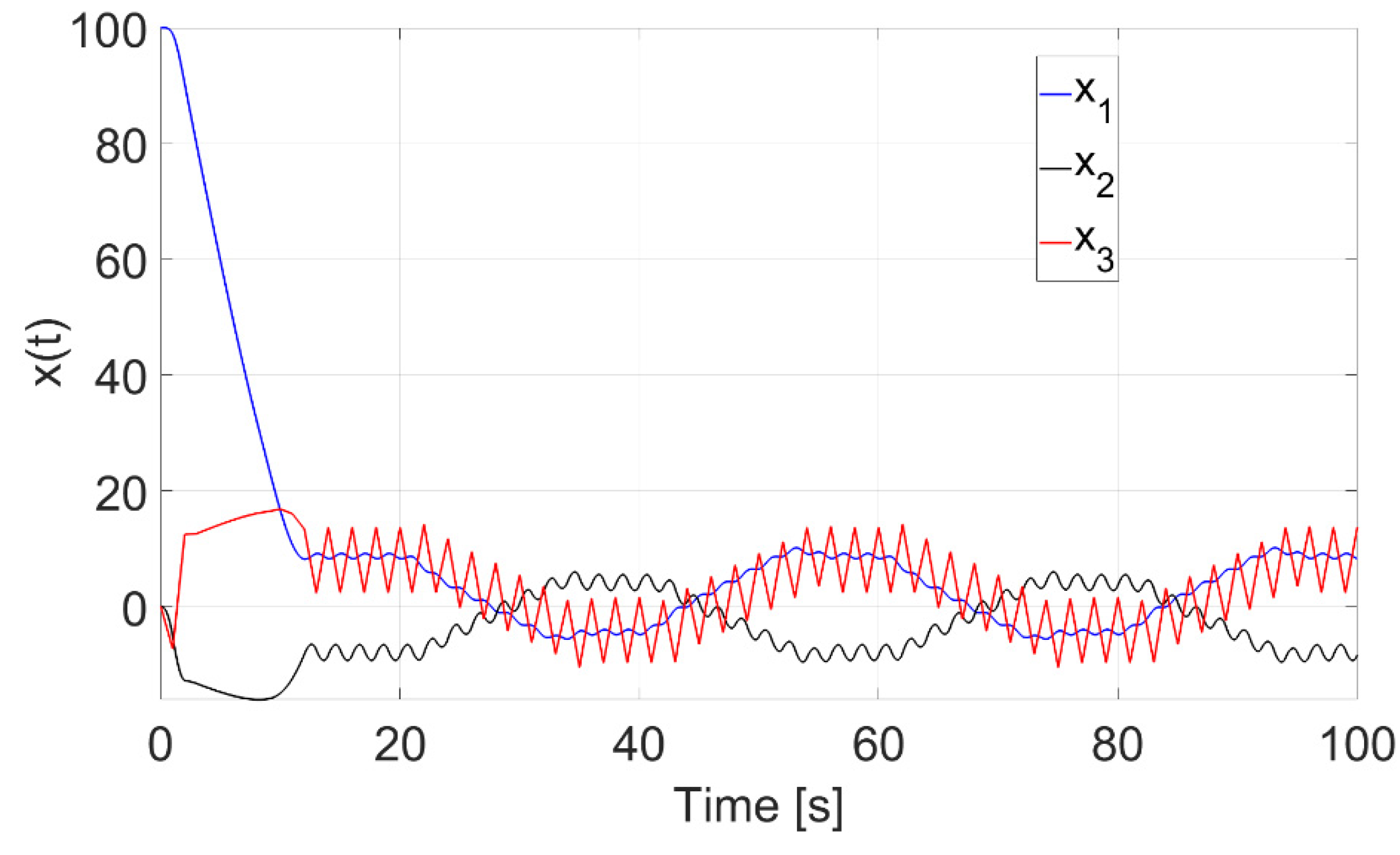
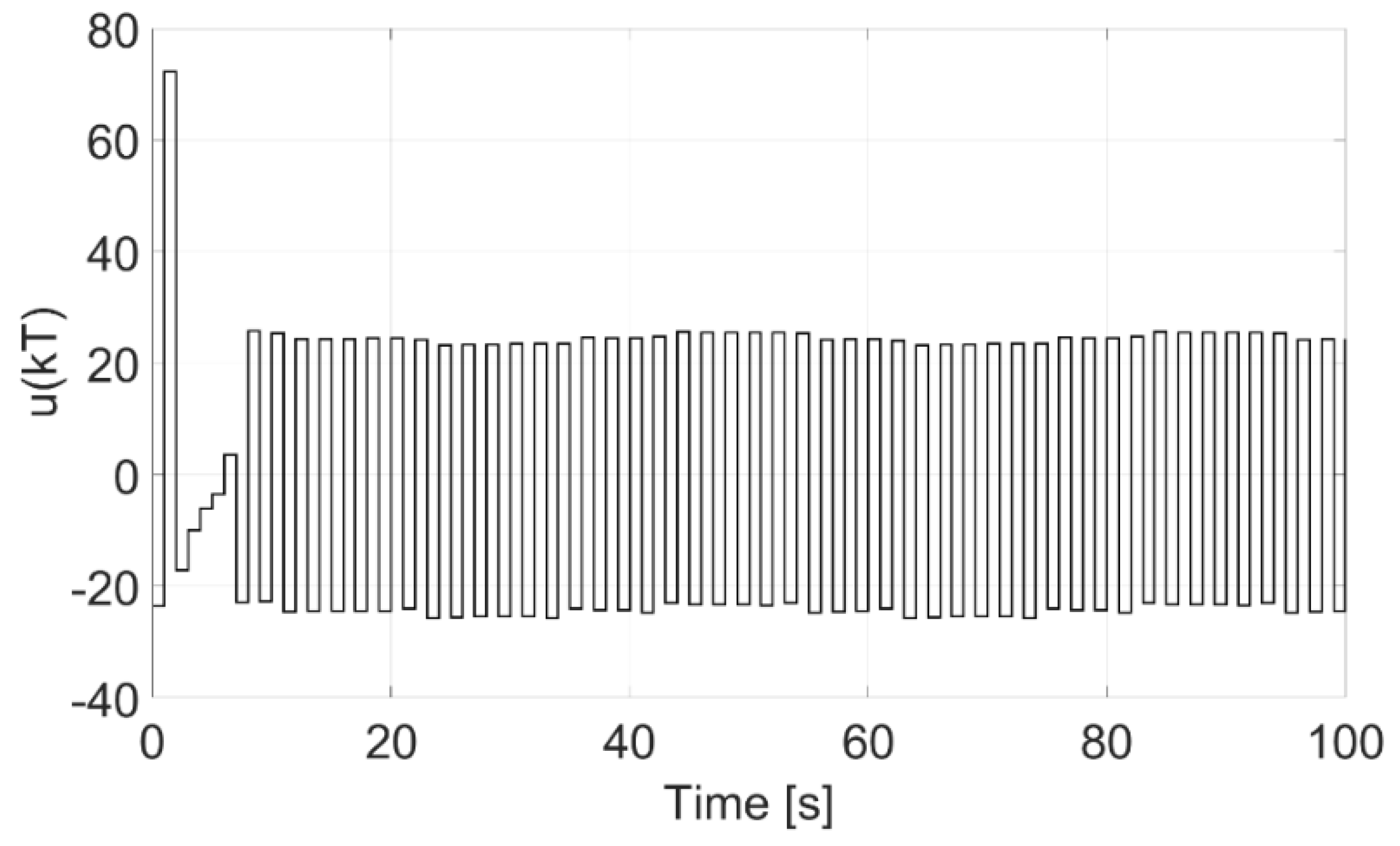
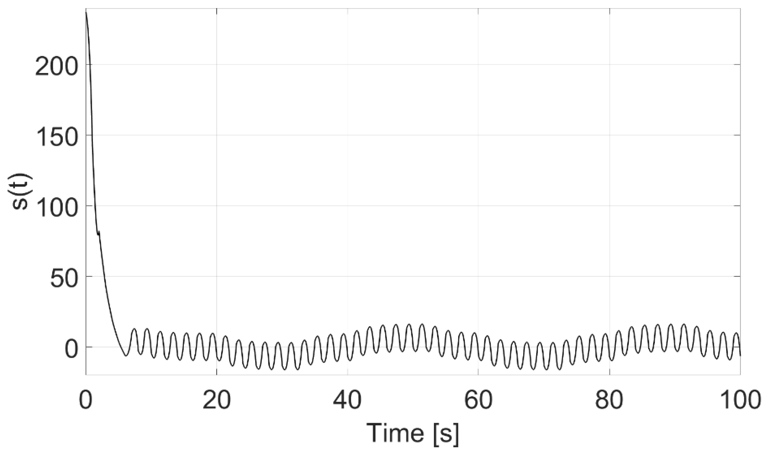
6.1. Switching Reaching Law Based Sliding Mode Controller

The results obtained with the switching type reaching law will be presented. The parameters s₀, ε must satisfy (15). They have been selected as s₀ = 30 and ε = 3.41, as a compromise between chattering and initial control signal value. The results of simulations are presented in Figure 2, Figure 3 and Figure 4.

As one can observe from the figures, the sliding variable converges to the band of a radius 5.78 obtained in Theorems 1 and 2 in finite time, and once it reaches this band it does not leave it for the rest of the control process. Using the switching reaching law based controller, the state is guaranteed to lie exactly on the sliding line, at least once in each discretization period, as was predicted in Theorem 3. Moreover, the convergence to the quasi-sliding mode band is faster. However, the drawback is a large magnitude of chattering. As one can observe, because the matching conditions are not satisfied, a constant disturbance leads to a steady state error. The impact of a constant disturbance could easily be removed by introducing an integral action into the switching hyperplane, which is not presented here for brevity. This error however is bounded, in accordance with Theorem 7.

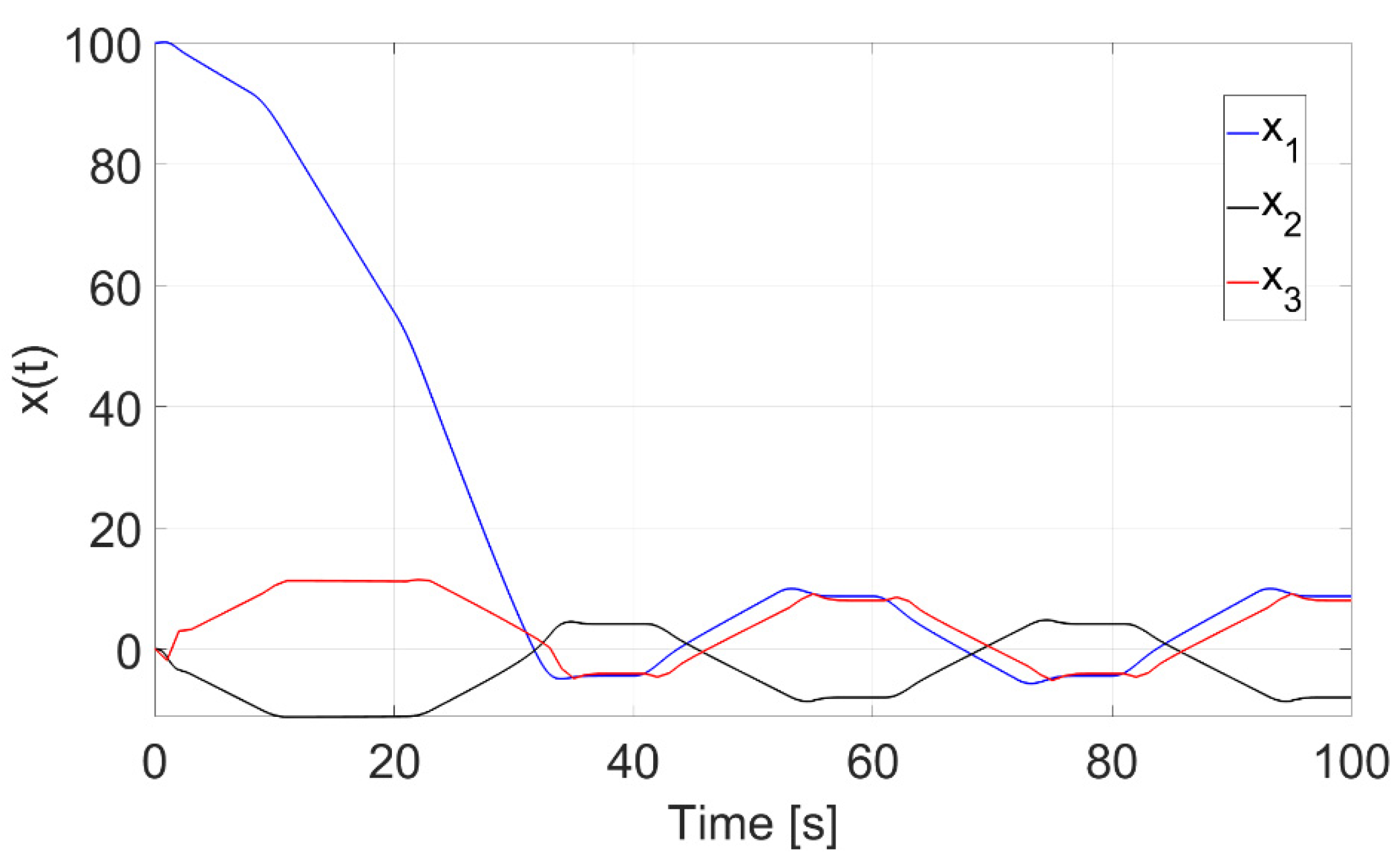
6.2. Non-Switching Reaching Law Based Sliding Mode Controller

Next, the results obtained with the non-switching reaching law will be presented. The single parameter s₀ must be selected as greater than s_d in order to ensure the existence of the sliding motion. Consequently it is selected as s₀ = 8 to obtain a compromise between initial value of the control signal and convergence speed. The results of simulations are presented in Figure 5, Figure 6 and Figure 7. As one can observe, the state converges to the vicinity of the sliding line. Moreover, once the quasi-sliding motion starts, the sliding variable never exceeds the value 3.36 predicted in Theorem 4. Similarly as in the previous case, the constant disturbance leads to a steady state error, which could be removed by introducing an integral action in the sliding variable equation. However, the state errors remain bounded, according to Theorem 7.

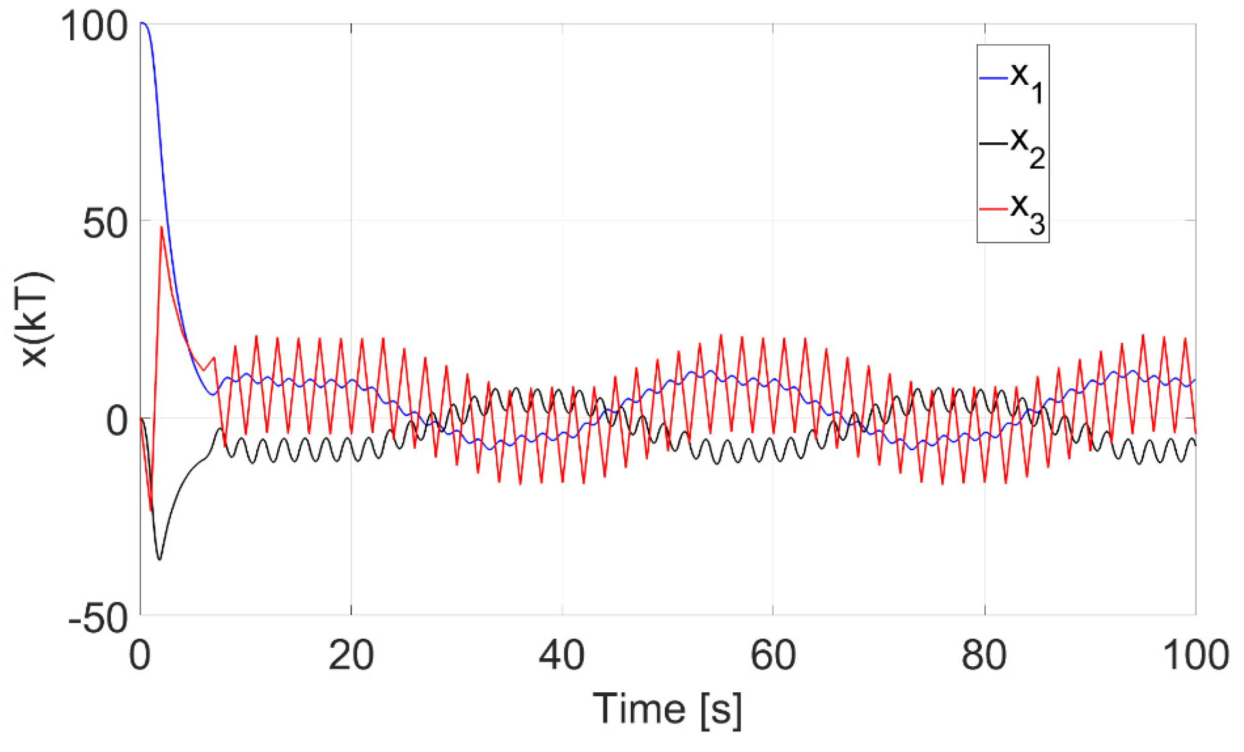
6.3. Gao’s Reaching Law Based Sliding Mode Controller

Next, we will compare our approach with the one proposed in the seminal work [16]. The reaching law developed in that paper is still widely used both in original as well as modified forms. Firstly, we have tried to apply Gao’s reaching law in its original form, however this resulted in significant chattering, as the discontinuous term had to compensate the whole disturbance magnitude. Therefore, to obtain a fair comparison with the reaching laws developed in this paper, we have modified the reaching law of Gao by introducing the disturbance compensation term. Thus the modified reaching law is:

$$s\left[\left(k+1\right)T\right]=\left(1-q\right)s\left(kT\right)-\epsilon \mathrm{sgn}\left[s\left(kT\right)\right]+c^T\left\{\mathit{d}\left(kT\right)-\mathit{d}\left[\left(k-1\right)T\right]\right\}.$$

(62)

The parameters q, ε have to be chosen in order to on one hand ensure the switching quasi-sliding motion, and on the other generating admissible control signal values. The parameter q mainly governs the initial rate of convergence, therefore it has a larger impact on the initial control signal. The value ε must be sufficiently large to ensure crossing the sliding hyperplane. These parameters were chosen as q = 0.36, ε = 11. The results are shown in Figure 8, Figure 9 and Figure 10.

Obviously, to ensure a fair comparison, the above parameters must be properly chosen. One can observe from Figure 10 that for the given value of q, the value of ε could not be decreased, as it is currently “just enough” to make the sliding variable change its sign in each consecutive step of the quasi-sliding motion. On the other hand, one could select a larger value of q, which would allow decreasing ε, and consequently reducing the chattering. This however would increase the initial values of the control signal, which are already significantly larger than the ones generated by the proposed controllers. Thus, one can notice, that both of the proposed reaching laws outperform Gao’s reaching law, not only in terms of smaller chattering but in reduced control effort as well.

6.4. Comparison of the Performance of the Controllers

When comparing the controllers, one of the most important aspects is the energy expenditure connected with the control signal. The sum of squared values was selected as a measure of this energy cost. On the other hand, every controller should minimize the state error. In the simulation scenario, the desired state is the origin of the state space, therefore minimizing the error is equivalent to minimizing the values of state variables. Thus, the sum of absolute values of the states given by ${\displaystyle \sum \left(\left|x_1\right|+\left|x_2\right|+\left|x_3\right|\right)}$ was used as a measure of control precision. The results are presented in

Table 1. Comparison of the controllers.

	Switching RL	Non-Switching RL	Gao’s RL
${\displaystyle \sum u^2\left(k\right)}$	11,259	437	61,589
${\displaystyle \sum \left(\left|x_1\right|+\left|x_2\right|+\left|x_3\right|\right)}$	2438	2371	2812

.

It is evident that both controllers proposed in this paper ensure reduced control effort and improved control precision, when compared to the reaching law developed by Gao, despite introducing the disturbance compensation term in it (without it, the difference would be even more significant). Moreover, the non-switching reaching law outperforms the switching one in both of the above-mentioned aspects.

7. Discussion

In this work, control of a continuous time plant by a discrete sliding mode controller was considered. Two reaching laws were proposed, one ensured the switching sliding motion, while the other the non-switching one. It has been shown, that the transition to a non-switching reaching law allows to significantly reduce the energy expenditure of the control signal. In both of the approaches, it was assumed that the external disturbance rate of change is bounded. It is worth pointing out, that the proposed approach does not require satisfying the matching conditions. Both controllers lead to a quasi-sliding mode band width (therefore also to control precision) proportional to T². It is also worth pointing out that both of the proposed methods ensure a priori known bounds of the state errors, not only at the sampling instants, but also in the intervals between them. This has clear practical advantages, as it can ensure that the states will not exceed values that could damage the plant. Moreover, as for the majority of systems, the greatest efficiency is achieved at the desired operating point, this property can also be used to optimize the efficiency. The analytical results were verified by computer simulations.

One drawback of the proposed method is the requirement of knowing the limits of the disturbance rate of change in advance. Our future research will focus on removing this requirement, which could be achieved with adaptive control methods. Moreover, tests in real power electronic systems are also planned.