A Procedure to Calculate First-Order Wave-Structure Interaction Loads in Wave Farms and Other Multi-Body Structures Subjected to Inhomogeneous Waves

Abstract

A typical assumption when performing analytical, numerical, and experimental studies in wave–structure interaction in multi-body problems such as for wave farms and very large floating structures is the homogeneity of the wave field. Important interactions between the floating elements are dependent on the direction, amplitude, and phase of the waves acting on each. Then, wave homogeneity is probably unrealistic in near-shore areas where these installations are to be deployed. In the present work, an existing interaction method, which allows the use of standard boundary element diffraction codes for solving the first order wave structure linear potential for each unique geometry in the problem, is shown to be able to account for inhomogeneous sea states across the domain of a multi-body problem requiring only minimal modification to its implementation. A procedure to use the method to include arbitrary incoming undisturbed wave conditions at each body is presented. A verification study was done by using an artificial numerical configuration to mimic an inhomogeneous wave field in a standard diffraction code, which was used as a reference. The results obtained using the interaction-method based procedure are shown to be in excellent agreement with the reference ones. Furthermore, an example of frequency inhomogeneity of the wave field in a wave farm is shown and the effects on the motion amplitudes and absorbed power are presented illustrating the applicability of the procedure.

1. Introduction

Computing the wave structure interaction in a multi-body problem has a wide range of applications in many offshore and coastal engineering problems configurations. It is particularly relevant for two engineering design problems: large floating structures and offshore wave energy farms. In both, an array of submerged body elements is present and wave structure multi-body interaction exists. This interaction is two-fold: (1) wave systems that are the result of scattering of incoming waves in individual submerged elements, which recursively excite all the elements of the array; and (2) wave systems that radiate away from each element as a result of the element motion, which excite the other elements of the array. Therefore, the wave excitation forces on each element differ from an element in isolation and so do the wave induced motions and derived quantities.

1.1. Array Interaction in Large Floating Structures

Very large floating structure (VLFS) designs are typically composed of several floating bodies that are connected above the waterline by continuous structural elements or connected through flexible elements such as cables or hinges, giving way for a modular component design. The generic floating bridge in [1] is an example of the former with its 35 floating pontoons supporting a continuous bridge girder, while the large floating hydrocarbon storage facility in [2] is an example of the latter. VLFSs also tend to include a large number of similar floating bodies such as in the floating airport design in [3,4] with tens of floating elements. Inter floater wave-structure interaction effects can lead to amplification of wave run-ups, the appearance of wave trapping modes, and excitation of natural modes. All these phenomena can significantly reduce the efficiency of the installation by impeding its operability, and even lead to catastrophic structural failures if not properly accounted for.

1.2. Array Interaction in Offshore Wave Energy Farms

Offshore wave energy exploitation is expected to be implemented in the form of wave farms composed of many wave energy converters (WECs). These farms should be compact to reduce area occupation and costs.

The layout of the farm affects the behavior of the units including the energy harvested due to the devices’ hydrodynamic interactions. These can be constructive or destructive, depending on the layout of the farm and the incoming wave system. The q-factor is the ratio between the absorbed power of the farm and the power absorbed by the same number of WECs, each one in isolation. Optimized array layouts can result in a q-factor higher than 1, effectively doubling or more the power output. In ideal conditions (e.g., in narrow banded sea-states and optimally tuned devices), the q-factor can increase dramatically. Unfortunately, the q-factor is extremely sensitive to wave period and direction. Optimal configurations appear as peaks in the optimization hyperspace surrounded by vast valleys of destructive interference ones [5]. Additionally, it has been proven that optimal configurations for a given wave direction are necessarily accompanied by destructive interactions for other wave headings [6]. Here, it is worth noting that, to the best of the author’s knowledge, wave farm studies so far do not take into account changes in the layout occurring from steady and low-frequency wave drift motions that may disturb optimal layouts. Nor do they consider variable local wave conditions throughout extensive wave farms. It is also important to bear in mind that dangerous phenomena similar to the ones described in Section 1.1 are also possible in wave farms.

1.3. The Direct Method

From the above, it should be evident that a proper identification of the interaction characteristics is paramount in the design spiral of VLFSs and wave farms for assuring an efficient and safe installation. Fast numerical methods are then needed and linear wave-structure diffraction codes implementing a boundary element approach (BEM) in the frequency domain are typically used, for example, WAMIT [7] and NEMOH [8] may be used when current is not considered, whereas HYDROSTAR [9] and MULDIF [10] can consider the effect of current with different degrees of accuracy.

The above codes solve the interaction problem by considering all the bodies as part of a boundary value problem for the oscillating potential flow solution–usually denominated the direct method. The computational burden can be reduced if one or two symmetry planes exist in the array of bodies, where only half or a quarter of the elements needs to be explicitly considered. However, in addition to the usually unrealistic restriction of symmetry limitation, this comes at the expense of redefining the problem into problem specific non-standard (symmetric or anti–symmetric) modes of motion. It then presents difficulties for further utilization of the results in time-domain codes (e.g., SIMO [11]) where nonlinear forces can be added under a weakly linear approach. When the number of bodies is in the order of tens or hundreds and the geometry of the bodies is not simple, the computational burden becomes prohibitive for a standard PC and inefficient for design optimization procedures when using a typical modern workstation.

1.4. Matrix Methods

In order to circumvent the aforementioned limitations, [12] developed an interaction theory for the computation of wave excitation forces for arrays of bodies that is exact within the limits of linear wave theory and accounts for both the evanescent and progressive wave systems. The method requires the knowledge of the hydrodynamic properties only for each unique body geometry as opposed to all the bodies in the direct method, giving way for significant computational savings. The interaction effects are introduced by resorting to algebraic relations that express the notion that waves scattered or radiated by one body are incident waves on the others. The procedure involves a diffraction transfer matrix, unique to each unique body geometry in the array in isolation, that transforms incident waves to the body in the corresponding scattered waves. However, both these wave systems are expressed as vectors of cylindrical partial-wave coefficients. This seriously undermines the applicability of the theory, as standard diffraction codes such as the ones mentioned in Section 1.3, which use planar waves in their formulation, cannot be used to compute the diffraction transfer matrix for bodies of arbitrary geometry. For this reason, application of this method is usually relegated in favor of the direct method, which is available in publicly available codes or commercial software. Despite this, important developments and applications of the method to arrays of bodies should be mentioned. Such are the ones by [13,14,15], considering the analytic solution of arrays of cylindrical bodies; and [16,17], considering axisymmetric and arbitrary body geometries, respectively, to compute the diffraction matrix.

More recently, ref. [18] presented a method to determine the necessary cylindrical partial-wave coefficients for an arbitrary geometry from information of the wave potential contained in a wet control surface surrounding the body. This method was then applied in [19] for deriving a diffraction transfer matrix from plane incident waves and where a new operator—the force transfer matrix—is formulated. The method presented in [19] effectively allows the usage of standard diffraction codes as input to the interaction methods originated by [12]. It does not account for the evanescent waves in the immediate vicinity of the bodies nor is it formulated for infinitely deep water, but for practical purposes, the method holds remarkably well, as shown in [20,21].

1.5. Inhomogeneous Wave Environment Conditions

Another fundamental drawback of the direct method is its inability to consider prescribed arbitrary inhomogeneous wave environments as input to individual bodies in a multi-body problem, while still accounting correctly for the hydrodynamic interactions between them. On the other hand, inhomogeneous wave conditions are a realistic assumption and its effects relevant for VLFSs, as demonstrated by [22].

Accounting for inhomogeneity and diffraction interaction using standard BEM diffraction codes is stated as an open challenge by [23] on the subject of near shore VLFSs. As an example, consider the work by [24], who presented a scheme to include individual arbitrary wave conditions on individual pontoons of an end-anchored floating bridge (but neglected interaction), together with the study by [25] on pontoon interaction of the same bridge design (but who did not consider inhomogeneity). Also worth mentioning is the variable bathymetry consideration throughout a WEC array in [26]; however, the methodology was based on a non-standard dedicated BEM formulation for computing the flow.

The need for accounting for inhomogeneous wave conditions in studies of WEC farms was reported in [19]. This is obviously particularly important when analyzing diffracted wave patterns in light of array layout analysis and optimization, as the coherent wave crest phases are artificial and lead to inaccurate outputs. Then, phase resolving models for wave climates become necessary as additional input if the study is purely numerical.

1.6. The Present Study

The need for considering inhomogeneous wave conditions in fast numerical simulations for some important multi-body problems has been identified. Irrespective of this, and to the best of the author’s knowledge, no methodology has been published in the literature explicitly demonstrating how to achieve it, or published studies where it has been applied.

In the work herein presented, it is shown that the interaction methodology in [19] can be exploited to account for wave inhomogeneity in multi-body problems with minimal modification of the procedure. The original method characteristics are kept, but there is a need to run the matrix method for each prescribed special distribution of local undisturbed incoming wave amplitude, direction, period, and phase, throughout the domain of interest, and change the implementation to account for inhomogeneous wave headings.

The problem formulation, interaction theory, and practical procedures are presented in Section 2. The verification and an illustrative example of application is given in Section 3 for a set of five bodies, which can be considered as wave energy converters. Discussion and overall conclusions, including further suggested work, are presented in Section 4.

2. Methodology

The problem formulation and methodology follow the ones presented in [7,12,19], but have been adapted to the consideration of inhomogeneous environmental waves, for which some nomenclature modification is required. Derivation of equations present already in the aforementioned references are omitted here to avoid repetition. Only the final expressions are presented and modified for the specific problem of the wave inhomogeneity, where necessary.

2.1. The Direct Method

Consider the problem of N bodies submerged in a fluid that is considered inviscid and incompressible. The fluid flow in the presence of waves is described by harmonically varying velocity potentials, ${\varphi }_j$, in the vicinity of each body j:

$${\varphi }_j\left(\mathit{x},t\right)=Re\left\{{\phi }_j\left(\mathit{x}\right)e^{i\omega t}\right\},$$

(1)

where $\omega$ is the angular frequency; $t$ denotes time; and $\phi$ is the complex potential at the point with cartesian coordinates $\mathit{x}=\left(x,y,z\right)$ satisfying the Laplace equation: ${\nabla }^2\phi = 0$. $\phi$ only needs to be valid in the interior of the domain delimited by the still water surface, the rigid bodies’ surfaces, the horizontal bottom, and an arbitrary cylindrical surface surrounding each body. The dispersion relation for linear progressive water waves is satisfied:

$$k_j=2\pi /{\lambda }_j={\omega }^2/\left(g·\tanh k_{j}h\right),$$

(2)

where ${\lambda }_j$ is the wavelength; $k_j$ is the wave number; $g$ stands for the standard gravity acceleration; and $h$ is the water depth. The total potential is obtained from the sum of the solutions of two boundary problems targeting the solution of the radiation potential, ${\phi }_j^R$ and the diffraction potential, ${\phi }_j^D$:

$${\phi }_j={\phi }^R+{\phi }_j^D={\phi }_j^R+\left({\phi }_j^0+{\phi }_j^S\right),$$

(3)

where ${\phi }_j^S$ is the disturbance potential, or scattering potential, due to the presence of all the bodies. ${\phi }_j^0$ is the undisturbed linear potential of a regular plane wave of amplitude $A_j$ propagating through body j at an angle ${\beta }_j$ with the $\mathit{x}=\left(1,0,0\right)$ vector and is expressed by:

$${\phi }_j^0=ig{A}_j/\omega ·\cosh k_j\left(z+h\right)/\cosh k_{j}h·\exp \left\{-ikx\cos {\beta }_j-iky\sin {\beta }_j\right\}.$$

(4)

The radiation potential is dependent on each ${\phi }_{q_j}$ potential, which denotes the potential corresponding to the flow induced by a unit amplitude harmonic velocity in the $q_j$ mode of the jth body. It is valid everywhere in the fluid and given by:

$${\phi }^R=i\omega {{\displaystyle \sum }}_{j=1}^{\mathit{n}}{{\displaystyle \sum }}_{q_j}^{Q_j}{\xi }_{q_j}{\phi }_{q_j}^R,$$

(5)

where ${\xi }_{q_j}$ is the complex amplitude in the $q_j$ mode. The following body boundary conditions for the two problems are applied to the mean wet surfaces of each body:

$$\partial {\phi }_j^D/\partial \mathit{n}=0 ; \partial {\phi }_{q_j}^R/\partial \mathit{n}={\mathsf{{\rm N}}}_{q_j},$$

(6)

where $\mathit{n}$ is the body surface normal and $n_{q_j}={\mathit{V}}_{{\mathit{q}}_{\mathit{j}}}·\mathit{n}$, with ${\mathit{V}}_{{\mathit{q}}_{\mathit{j}}}$ denoting the unit displacement vector of the mode $q_j$. If ${\beta }_j=\beta \wedge A_j=A$, $j=1,\dots ,N$, then ${\phi }_j^0={\phi }^0$ and ${\phi }_j^D={\phi }^D$, thus forming a consistent solution valid everywhere in the fluid. The problems can then be solved using Green’s second and third entities to formulate the following integral equations for the radiation and diffraction potentials:

$$2\pi {\phi }_{q_j}^R\left(\mathit{x}\right)+{{\displaystyle \int }}_{S_b}^{}{\phi }_{q_j}\left({\mathit{P}}_s\right)·\partial G\left(\mathit{x},{\mathit{P}}_s\right)/\partial n_{q_j}ds={{\displaystyle \int }}_{S_b}^{}{N}_{q_j}·G\left(\mathit{x},{\mathit{P}}_s\right)ds,$$

(7)

$$2\pi {\phi }_D\left(\mathit{x}\right)+{{\displaystyle \int }}_{S_b}^{}{\phi }_D\left({\mathit{P}}_s\right)·\partial G\left(\mathit{x},{\mathit{P}}_s\right)/\partial n_{q_j}ds=4\pi {\phi }_0.$$

(8)

In Equations (7) and (8), ${\mathit{P}}_s$ is a point in the surface $S_b$ of all the bodies together and $G\left(\mathit{x},{\mathit{P}}_s\right)$ is the green function denoting the potential at $\mathit{x}$ due to a point source of strength $-4\pi$ located at ${\mathit{P}}_s$. Then, using the linearized Bernoulli equation, the radiation and diffraction pressures are attained. From these, motions and other response amplitude operators can be obtained (see [7] for details).

Equations (7) and (8) are the integral equations used by standard boundary element method diffraction codes for the solution of the linear problem. It is evident that Equation (8) does not allow for different incoming wave amplitudes or directions to be prescribed to the different bodies. On the other hand, it is trivial to acknowledge that the problem can be solved for each body in isolation, which has been pursued by [24,27], but then no interaction is accounted for. Therefore, if one wishes to take advantage of these codes, an external inhomogenizing procedure must be applied while taking advantage of the computations for an isolated body: this can be achieved by the solution of an interaction problem.

2.2. The Interaction Problem

The potential of a planar wave hitting the body j can be expressed in cylindrical coordinates $\left(r_j,{\theta }_j,z\right)$ with the origin on the center of the body, using the relation ${\left(x-X,y-Y\right)}_j=r_j\left(\cos \theta ,\sin \theta \right)$, where ${\left(X,Y\right)}_j$ are the horizontal cartesian coordinates of the centre of body j. The representation is as follows:

$${\phi }_j^0\left(h,{\beta }_j,r_j,{\theta }_j,z\right)=ig/\omega \left({\mathit{a}}_{\mathit{j}}^{\mathbf{0}}·{\Psi }_{\mathit{j}}^{\mathbf{0}}\right),$$

(9)

where ${\mathit{a}}_{\mathit{j}}^{\mathbf{0}}$ and ${\Psi }_{\mathit{j}}^{\mathbf{0}}$ are vectors with an infinite number of m elements including m = 0. These are defined by:

$${\left\{{\mathit{a}}_{\mathit{j}}^{\mathbf{0}}\right\}}_m=\left[A_j·\exp \left\{-i{\epsilon }_j\right\}\right]·\exp \left\{-i\left[m\left({\beta }_j+\pi /2\right)\right]\right\}$$

(10)

$${\left\{{\Psi }_{\mathit{j}}^{\mathbf{0}}\right\}}_m=J_m\left(k_j{r}_j\right)·e^{\left(im\theta \right)}·\cosh k_j\left(h+z\right)/\cosh k_{j}h,$$

(11)

where $J_m$ is the mth order Bessel function of the first kind, rendering ${\Psi }_{\mathit{j}}^{\mathbf{0}}$ as a vector of (incoming) basis functions, and ${\epsilon }_j$ is the prescribed undisturbed wave phase angle at the center of body j. Note that ${\epsilon }_j$ is only a measure of the origin of the wave when there is only one body and that it is equal to ${\epsilon }_0=k\left(X_j\cos \beta +Y_j\sin \beta \right)$ for the case of homogeneous undisturbed plane waves. For the radiated and scattered potentials, one has:

$${\phi }_j^{R;S}\left(h,{\beta }_j,r_j,{\theta }_j,z\right)=ig/\omega \left({\mathit{a}}_{\mathit{j}}^{\mathit{S};\mathit{R}}·{\Psi }_{\mathit{j}}^{\mathit{S}}\right),$$

(12)

where ${\mathit{a}}_{\mathit{j}}^{\mathit{S}}$ depends on the geometry of each body and ${\mathit{a}}_{\mathit{j}}^{\mathit{R}}$ also on the mode of motion, being both infinite vectors of coefficients. ${\Psi }_{\mathit{j}}^{\mathit{S}}$ is a vector of (scattering) basis functions. While the phase information of the undisturbed waves is prescribed in Equation (10), the same needs to be solved for the radiation and scattering problems. Therefore, the Hankel function is used instead of the Bessel function to include both real and imaginary parts in the definition of ${\Psi }_{\mathit{j}}^{\mathit{S}}$:

$${\left\{{\Psi }_{\mathit{j}}^{\mathit{S}}\right\}}_m=H_j^{\left(2\right)}\left(k_j{r}_j\right)·e^{\left(im\theta \right)}·\cosh k_j\left(h+z\right)/\cosh k_j{h}_j,$$

(13)

where $H_j^{\left(2\right)}$ stands for the Hankel function of the second kind of order m. Note that the infinite vectors in Equation (9) through Equation (13) can be truncated to $-M<m<+M$, making way for an approximation with arbitrary precision, which is used herein.

From the sum of the undisturbed wave at body j with the incoming scattered waves at body j (from the other bodies), one defines the incident wave potential on body j:

$${\phi }_j^I=ig/\omega ·\left({\mathit{a}}_{\mathit{j}}^{\mathbf{0}}·{\Psi }_{\mathit{j}}^{\mathbf{0}}+{{\displaystyle \sum }}_{\begin{array}{c}p=1\\ j\ne p\end{array}}^N{\mathit{a}}_{\mathit{p}}^{\mathit{S}}·{\Psi }_{\mathit{p}}^{\mathit{S}}\right).$$

(14)

Introducing a transformation matrix ${\mathit{T}}_{\mathit{j}\mathit{p}}$, so that ${\Psi }_{\mathit{p}}^{\mathit{S}}={\mathit{T}}_{\mathit{j}\mathit{p}}\times {\Psi }_{\mathit{j}}^{\mathit{S}}$, Equation (14) becomes:

$${\phi }_j^I=ig/\omega ·\left({\mathit{a}}_{\mathit{j}}^{\mathbf{0}}+{{\displaystyle \sum }}_{\begin{array}{c}p=1\\ j\ne p\end{array}}^N{\mathit{T}}_{\mathit{j}\mathit{p}}{}^T\times {\mathit{a}}_{\mathit{p}}^{\mathit{S}}\right)·{\Psi }_{\mathit{j}}^{\mathbf{0}}.$$

(15)

It is important to note that ${\mathit{T}}_{\mathit{j}\mathit{p}}$ is the actual transformation matrix with shape $\left(2M+1\right)\times \left(2M+1\right)$, whereas the indexing $jp$ denotes the pair of bodies to which these elements are to be applied—the elements $\left(2M+1\right)\times \left(2M+1\right)$ are specific for each pair. Using Graf’s addition theorem ([19,28]), the mnth element of the matrix comes:

$${\left\{{\mathit{T}}_{\mathit{j}\mathit{p}}\right\}}_{\mathit{m}\mathit{n}}=H_{m-n}^{\left(2\right)}\left(k{L}_{jp}\right)·\exp \left\{i\left(m-\mathit{n}\right){\alpha }_{jp}\right\},$$

(16)

where:

$$L_{jp}=\sqrt{{\left(X_j-X_p\right)}^2+{\left(Y_j-Y_p\right)}^2},$$

(17)

$${\alpha }_{jp}=\mathrm{atan}\left(Y_j-Y_p\right)/\left({\mathit{x}}_j-{\mathit{x}}_p\right).$$

(18)

A diffraction transfer matrix ${\mathit{D}}_{\mathit{j}}$ can be defined that transforms incident wave amplitudes to body j into scattered wave amplitudes from the same body. Then, the scattered wave amplitudes that are required to determine the potential in Equation (15) can be obtained from the solution of the following system of linear equations:

$${\mathit{a}}_{\mathit{j}}^{\mathit{S}}={\mathit{D}}_{\mathit{j}}\times \left({\mathit{a}}_{\mathit{j}}^{\mathbf{0}}+{{\displaystyle \sum }}_{\begin{array}{c}p=1\\ j\ne p\end{array}}^N{\left[{\mathit{T}}_{\mathit{j}\mathit{p}}\right]}^T\times {\mathit{a}}_{\mathit{p}}^{\mathit{S}}\right),$$

(19)

where ${\mathit{D}}_{\mathit{j}}$ is a vector of N elements, each element being a matrix with the shape $\left(2M+1\right)\times \left(2M+1\right)$, corresponding to each jth body.

For the radiation problem, the formulation is similar, but replacing ${\mathit{a}}_{\mathit{j}}^{\mathbf{0}}$ with ${\mathit{a}}_{\mathit{j},{\mathit{q}}_{\mathit{p}}}^{\mathbf{0}}$ as follows:

$${\mathit{a}}_{\mathit{j},{\mathit{q}}_{\mathit{p}}}^{\mathbf{0}}=\left\{\begin{array}{cc}{\mathit{T}}_{\mathit{j}\mathit{p}}{}^T\times {\mathit{a}}_{{\mathit{q}}_{\mathit{p}}}^{\mathit{R}}& if j\ne p\\ \mathbf{0}& if j=p\end{array}\right..$$

(20)

At this point, it should be clear that at no point in the interaction theory presented does the undisturbed incident wave filled at the bodies needs to be equal in amplitude, direction, or the phase equal to ${\epsilon }_0$. The modification relative to [19,12] herein implemented is to consider prescribed and possibly independent $A_j$, ${\beta }_j$, and ${\epsilon }_j$ for each jth body, instead of $A,\beta$, and ${\epsilon }_0$ starting from Equation (9).

2.3. Excitation Forces and Hydrodynamic Coefficients

In a similar way to the diffraction transfer matrix, a force transfer matrix ${\mathit{G}}_{\mathit{j}}$ can be defined as a linear operator that transforms incident linear waves to body j into linear excitation forces in body j. Then, the excitation forces due to undisturbed incident planar waves on the jth body come:

$${\mathit{F}}_{\mathit{j}}^{\mathit{E}}={\mathit{G}}_{\mathit{j}}\times \left({\mathit{a}}_{\mathit{j}}^{\mathbf{0}}\left(A_j,{\beta }_j,{\epsilon }_j\right)+{{\displaystyle \sum }}_{\begin{array}{c}p=1\\ j\ne p\end{array}}^N{\mathit{T}}_{\mathit{j}\mathit{p}}{}^T\times {\mathit{a}}_{\mathit{p}}^{\mathit{S}}\right),$$

(21)

where ${\mathit{F}}_{\mathit{j}}^{\mathit{E}}$ is a $Q_j\times 1$ vector and ${\mathit{G}}_{\mathit{j}}$ is a $Q_j\times \left(2M+1\right)$ matrix. The radiation problem solution for computing the hydrodynamic coefficients does not depend on the incoming wave system, so the formulation is kept exactly the same as in [19]:

$${\left\{{\mathit{F}}_{\mathit{j}}^{\mathit{R}}\right\}}_{\ast q_p}=\left\{\begin{array}{cc}{\mathit{G}}_{\mathit{j}}\times \left({\mathit{T}}_{\mathit{j}\mathit{p}}{}^T\times {\mathit{a}}_{{\mathit{q}}_{\mathit{p}}}^{\mathit{R}}+{{\displaystyle \sum }}_{\begin{array}{c}p=1\\ j\ne p\end{array}}^N{\mathit{T}}_{\mathit{j}\mathit{p}}{}^T\times {\mathit{a}}_{\mathit{p}}^{\mathit{S}}\right)& if j\ne p\\ -{\omega }^2{\left[{\mathit{A}}_{\ast {\mathit{q}}_{\mathit{p}}}\right]}_{\mathit{p}}+i\omega {\left[{\mathit{B}}_{\ast {\mathit{q}}_{\mathit{p}}}\right]}_{\mathit{p}}+{\mathit{G}}_{\mathit{j}}\times {{\displaystyle \sum }}_{\begin{array}{c}p=1\\ j\ne p\end{array}}^N{\mathit{T}}_{\mathit{j}\mathit{p}}{}^T\times {\mathit{a}}_{\mathit{p}}^{\mathit{S}}& if j=p\end{array}\right.,$$

(22)

where ${\mathit{F}}_{\mathit{j}}^{\mathit{R}}$ is of shape $\left(Q_j\times Q\right)$ and ${\left\{{\mathit{F}}_{\mathit{j}}^{\mathit{R}}\right\}}_{\ast {\mathit{q}}_{\mathit{p}}}$ stands for its $q_p$th column. ${\left[A_{\ast q_p}\right]}_p$ and ${\left[B_{\ast q_p}\right]}_p$ correspond to the added mass and damping matrices q_pth columns of the body p in isolation. The complete radiation force matrix is then ${\mathit{F}}^{\mathit{R}}={\left\{{\mathit{F}}_{\mathbf{1}}^{\mathit{R}},{\mathit{F}}_{\mathbf{1}}^{\mathit{R}}, \dots , {\mathit{F}}_{\mathit{n}}^{\mathit{R}}\right\}}^T$ and the added mass matrix, $\mathit{A}$, and the wave radiation damping matrix, $\mathit{B}$, are given by:

$$\mathit{A}=-1/{\omega }^2·Re\left\{{\mathit{F}}^{\mathit{R}}\right\}$$

(23)

$$\mathit{B}=1/\omega ·Im\left\{{\mathit{F}}^{\mathit{R}}\right\}$$

(24)

2.4. Diffraction and Force Transfer Matrices from Standard Diffraction Codes

It is important to recall that these matrices are linear operators that transform incident cylindrical wave fields on a body into scattered wave fields, from the body, or forces, applied on the body. They are thus obviously independent of the wave field and are specified for each unique body geometry in isolation. Then, by considering a set of $\left(2M+1\right)$ incident plane wave directions on the jth body in isolation, ${\mathit{D}}_{\mathit{j}}$ and ${\mathit{G}}_{\mathit{j}}$ can be obtained from the systems of equations:

$$\left[\begin{array}{ccc}{a}_{{\beta }_1,-M}^S& \cdots & a_{{\beta }_{{\mathit{n}}^{\ast },-M}}^S\\ ⋮& \ddots & ⋮\\ a_{{\beta }_1,M}^S& \cdots & a_{{\beta }_{{\mathit{n}}^{\ast },M}}^S\end{array}\right]=\left[\begin{array}{ccc}{D}_{-M,0}& \cdots & D_{-M,M}\\ ⋮& \ddots & ⋮\\ D_{M,0}& \cdots & D_{M,M}\end{array}\right]\times \left[\begin{array}{ccc}{a}_{{\beta }_1,-M}^0& \cdots & a_{{\beta }_{{\mathit{n}}^{\ast }},-M}^0\\ ⋮& \ddots & ⋮\\ a_{{\beta }_1,M}^0& \cdots & a_{{\beta }_{{\mathit{n}}^{\ast }},M}^S\end{array}\right],$$

(25)

$$\left[\begin{array}{ccc}{F}_{q_1,{\beta }_1}^E& \cdots & F_{q_{1,{\beta }_{{\mathit{n}}^{\ast }}}}^E\\ ⋮& \ddots & ⋮\\ F_{{\beta }_1,M}^S& \cdots & a_{{\beta }_{{\mathit{n}}^{\ast },M}}^S\end{array}\right]=\left[\begin{array}{ccc}{G}_{q_1,-M}& \cdots & G_{q_1,M}\\ ⋮& \ddots & ⋮\\ G_{q_Q,-M}& \cdots & G_{q_Q,M}\end{array}\right]\times \left[\begin{array}{ccc}{a}_{{\beta }_1,-M}^0& \cdots & a_{{\beta }_{{\mathit{n}}^{\ast }},-M}^0\\ ⋮& \ddots & ⋮\\ a_{{\beta }_1,M}^0& \cdots & a_{{\beta }_{{\mathit{n}}^{\ast }},M}^S\end{array}\right],$$

(26)

where the body index has been dropped. In Equations (25) and (26), $a_{{\beta }_i,m}^{S;0}$ stands for the scattered, or incident, $m$th cylindrical partial wave amplitude coefficient resulting from an undisturbed incoming plane wave of unit amplitude with heading angle ${\beta }_i$. In Equation (26), $F_{q_i,{\beta }_j}^E$ stands for the excitation force in mode $q_i$ from an incoming undisturbed plane wave field with heading ${\beta }_i$. Equations (25) and (26) express a regression problem with both systems being underdetermined if $N^{\ast }<2M+1$ and overdetermined if $N^{\ast }>2M+1$. Realizing this, the actual angles to use should, in general, cover the range from 0 rad to $2\pi$ rad to avoid overfitting the coefficients within a small range. Furthermore, the larger is $N^{\ast }$, the better the quality of the obtained diffraction and force transfer matrices’ coefficients.

While $a_{{\beta }_i,j}^0$ can be determined from Equation (10), there is a need to have the information of the scattered wave amplitude coefficients to use in Equation (25). These are obtained from the following relation:

$$\begin{gathered} a_{{\beta }_j,m}^S=i\omega ·2\cosh \left(kh\right)/\left[2\pi gh·\left(1+\sinh \left(2kh\right)/2kh\right)·H_m^{\left(2\right)}\left(k{R}_i\right)\right] \\ \times {{\displaystyle \int }}_{-h}^0{{\displaystyle \int }}_0^{2\pi }{\phi }_{{\beta }_j}^S\left(R,\theta ,z\right)·\exp \left\{-im\theta \right\}·\cosh k\left(h+z\right)d\theta dz. \end{gathered}$$

(27)

${\phi }_{{\beta }_j}^S$ can be obtained numerically from the solution of Equation (8) and then determining the potential at a cylindrical surface centered at the body with radius $R$–denoted control surface from hereon. One should also bear in mind that only the progressive waves are taken into account, meaning that R should not be too close to the surface of the body for Equation (27) to be valid. Furthermore, the control surface of one body in the multi-body problem cannot intersect the surface of another body; on the other hand, control surfaces can intersect each other.

Finally, one needs the radiated wave coefficients to use in Equation (22). These are obtained from the radiation potential distribution on the same aforementioned control surface for each mode of motion $q_p$, as follows:

$$\begin{gathered} {\left\{{\mathit{a}}_{{\mathit{q}}_{\mathit{p}}}^{\mathit{R}}\right\}}_m=i\omega ·2\cosh \left(kh\right)/\left[2\pi gh·\left(1+\sinh \left(2kh\right)/2kh\right)·H_m^{\left(2\right)}\left(k{R}_i\right)\right] \\ \times {{\displaystyle \int }}_{-h}^0{{\displaystyle \int }}_0^{2\pi }{\phi }_{q_p}^S\left(R,\theta ,z\right)·\exp \left\{-im\theta \right\}·\cosh k\left(h+z\right)d\theta dz. \end{gathered}$$

(28)

The derivation of Equations (27) and (28) is essentially based on application of a Fourier transform to the velocity potential and consequent exploitation of the orthogonality of the depth dependent terms obtained. Details can be found in [18] and are not covered herein.

2.5. Practical Computational Procedures

Now that the theoretical aspects have been addressed, the practical steps involved in computation of the interaction problem are explained. Furthermore, a suggested stepwise approach for exploiting the results for arbitrary prescribed inhomogeneous spectra is presented.

The following lists the procedure to define a discrete inhomogeneous field for a multi-body diffraction problem using the interaction theory described in Section 2.2, Section 2.3 and Section 2.4:

• Impose an arbitrary directional wave variance spectrum at the location of each body including both amplitude and phase information.
• Optional: Define a reference location (e.g., the location of one of the bodies).
• Produce a 3-dimensional array $\widehat{\mathit{A}}$ with shape $N_b\times N_{\omega }\times N_{\beta }$, where $N_b$ is the number of bodies, $N_{\omega }$ is the number of frequencies, and $N_{\beta }$ is the number of wave headings in the entire spectral range of all bodies.

Populate $\widehat{\mathit{A}}$ with the complex incoming undisturbed wave amplitudes to each body (i.e., the complex vector representation of the term ${\left(A_j·\exp \left\{-i{\epsilon }_j\right\}\right)}_{b_j,{\omega }_k,{\beta }_m,}:j=1,\dots , N_b\wedge k=1,\dots , N_{\omega }\wedge m=1,\dots , N_{\beta }$,) in Equation (10).

Note that this defines the inhomogeneity of the wave environment and effectively produces a locked relation of the phases, amplitudes, and directions of the incoming undisturbed waves between all the bodies. If step 2 is implemented, the complex amplitudes can be made relative to a unit amplitude wave system with origin at the reference point.

The following lists the computational steps for acquiring the necessary single body hydrodynamic data for solving the interaction problem. All steps can be carried out using standard frequency domain diffraction codes:

4.

Compute the added mass, damping coefficients, and hydrostatic stiffness matrix (if motions are to be calculated) for each unique geometry in isolation. The hydrodynamic coefficients are used in Equation (22).

5.

Compute the excitation forces on each unique geometry in isolation considering a set of at least 2M + 1 (preferably more) incident wave headings covering the range 0 to $2\pi$ and the $N_{\omega }$ frequencies. The forces are used in Equation (26) to determine the force transfer matrix $\mathit{G}$.

6.

Compute the diffraction potential at a control surface surrounding each unique body geometry in isolation for a set of at least 2M + 1 (preferably more) incident wave headings covering the range 0 to $2\pi$ and the $N_{\omega }$ frequencies. The potential distribution at the control surface is used in Equation (27) to determine $a_{{\beta }_j,m}^S$, which then feeds Equation (25) to determine the diffraction transfer matrix $\mathit{D}$.

7.

Compute the radiation potential for each motion mode of each unique body geometry at the same control surface mentioned in the previous point. The potential distribution at the control surface is used in Equation (28) to determine ${\mathit{a}}_{{\mathit{q}}_{\mathit{p}}}^{\mathit{R}}$ to be applied in Equation (22).

The following lists the steps to acquire the multi-body hydrodynamic quantities:

8.

For each frequency ${\omega }_i, i=1,\dots , N_{\omega }$:

• Solve the system of linear equations in Equation (19) to determine the diffraction ${\mathit{a}}_{\mathit{j}}^{\mathit{S}}$ for each body and for each of the ${\beta }_N$ wave headings. Here, the corresponding element of $\widehat{\mathit{A}}$ needs to be used for each ${\mathit{a}}_{\mathit{j}}^{\mathit{0}}$.
• Compute the excitation forces for each body and for each of the ${\beta }_N$ wave headings using Equation (21).
• The excitation force on each body is the sum of the excitation forces applied on the body from all the ${\beta }_N$ angles.

9.

Solve the system of linear equations in Equation (19) with the substitution in Equation (20) to determine the radiation ${\mathit{a}}_{\mathit{j}}^{\mathit{S}}$ for each jth body and then compute the full multi-body added mass and damping coefficient matrices using Equations (22)–(24).

After step 9, the full coupled hydrodynamic quantities and excitation forces have been resolved for all the frequencies. Response amplitude operators can then be computed following the usual approaches, but it is important to stress that the amplitude relations between the incoming undisturbed wave fields between all the bodies must be maintained.

3. Results

This section presents the verification of the methodology presented in Section 2 using a special configuration of a diffraction problem using WAMIT for the inhomogeneous wave multi-body problem. An example of the case where frequency inhomogeneity is present is also shown and analyzed.

The freely available MATLAB code in [29] was modified to include wave inhomogeneity input and computation capability and then used for obtaining the interaction problem solution’s raw results in terms of hydrodynamic coefficients and excitation forces. Further pre- and post-processing and analysis were done using python scripts implemented by the author.

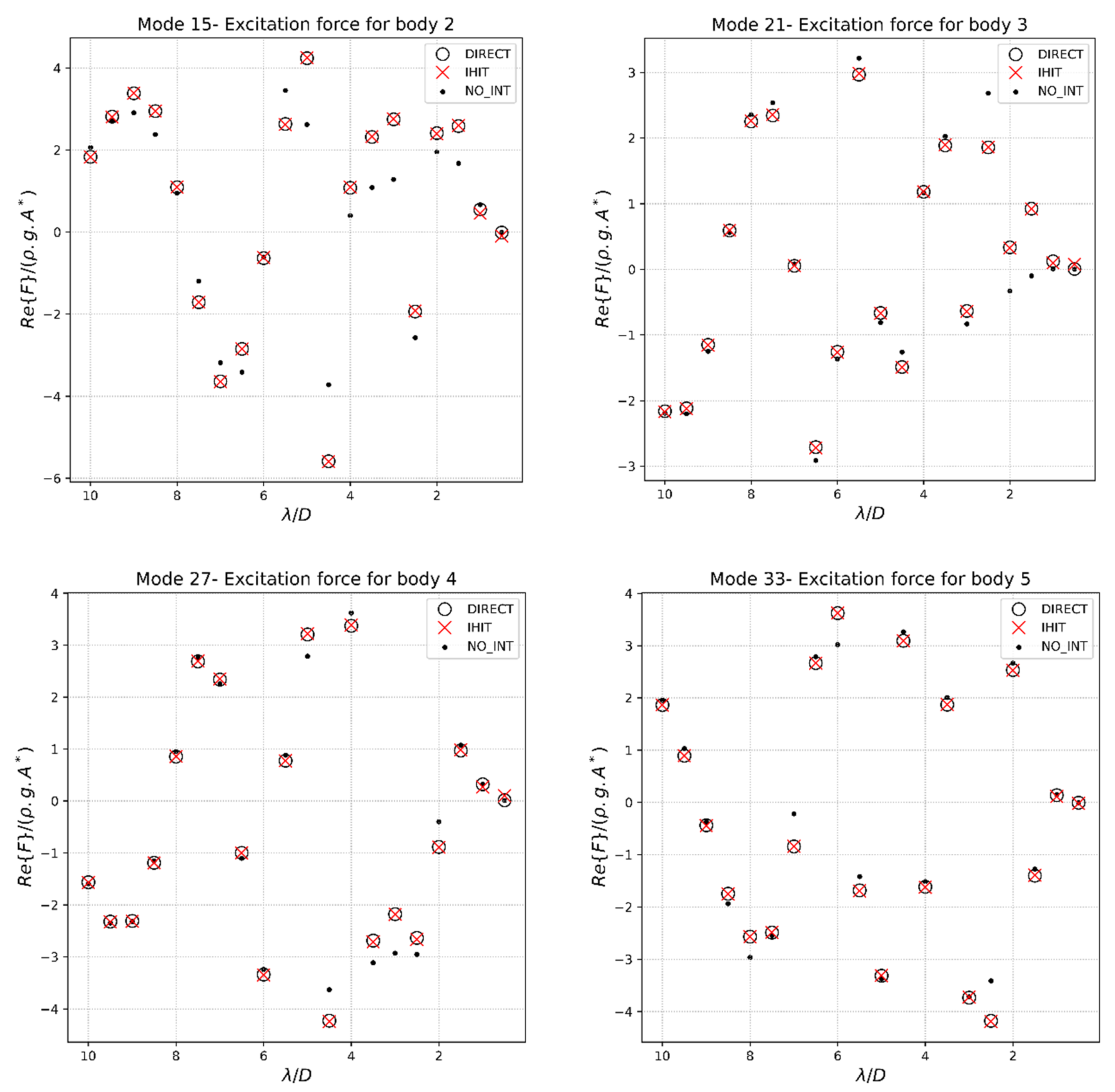
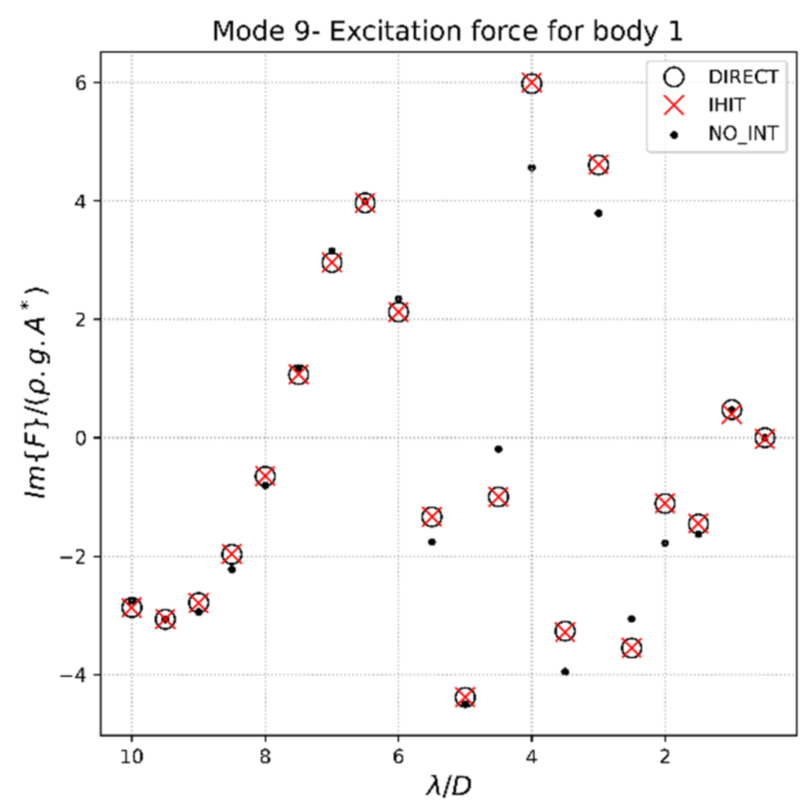
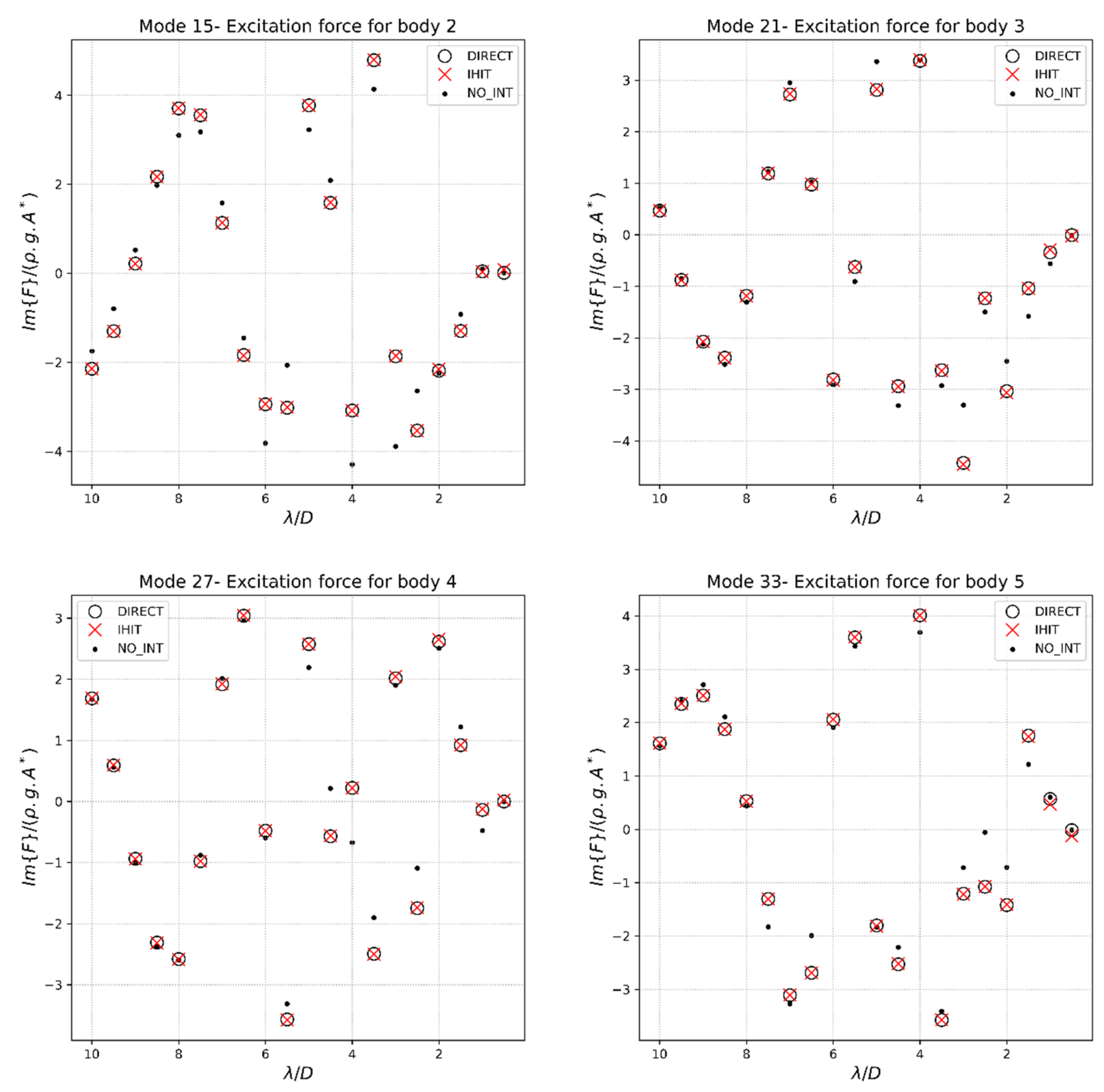
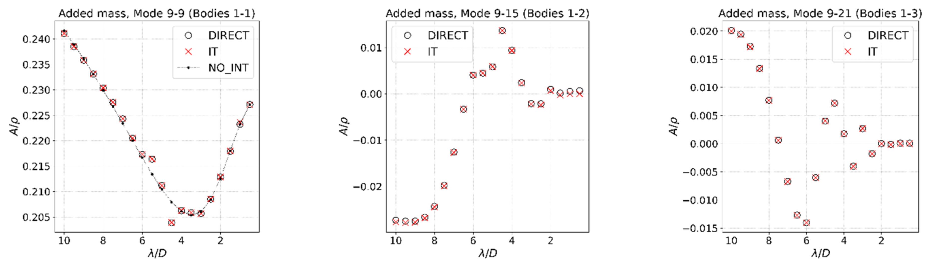
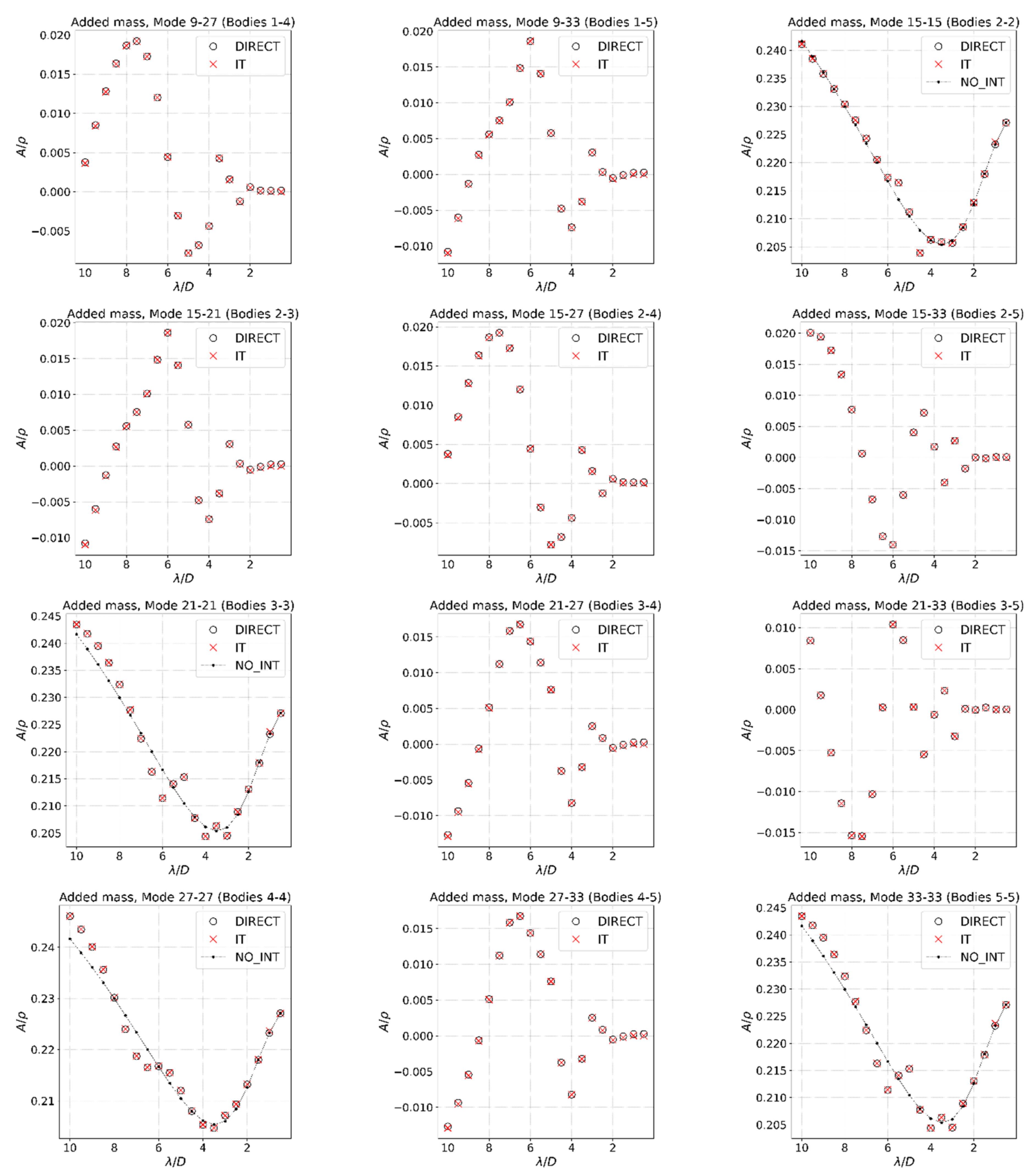
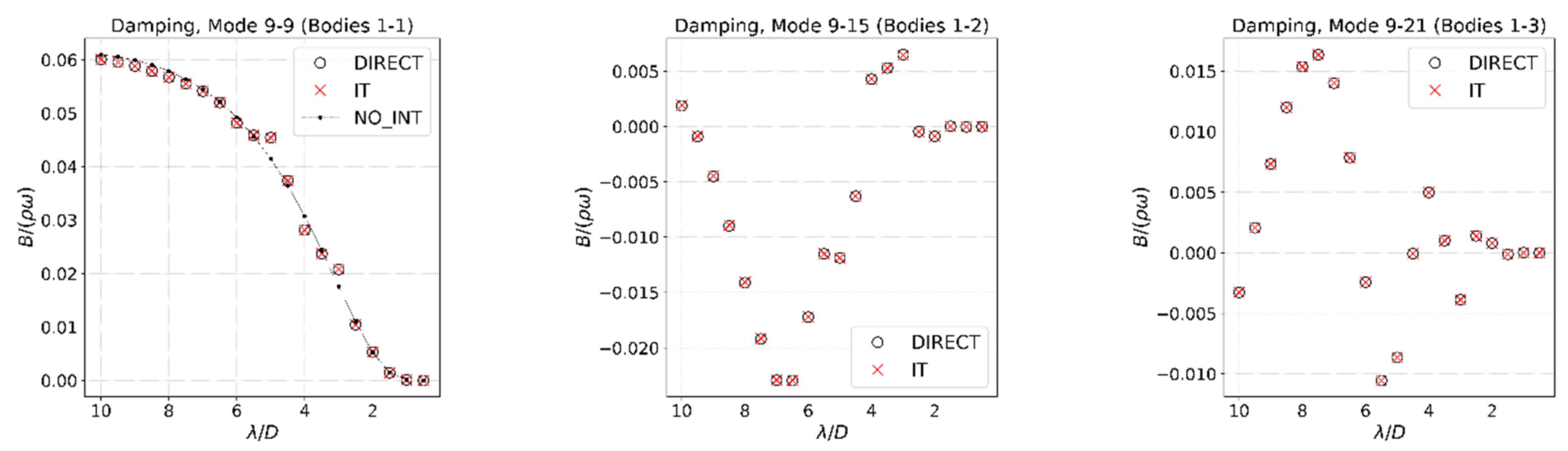
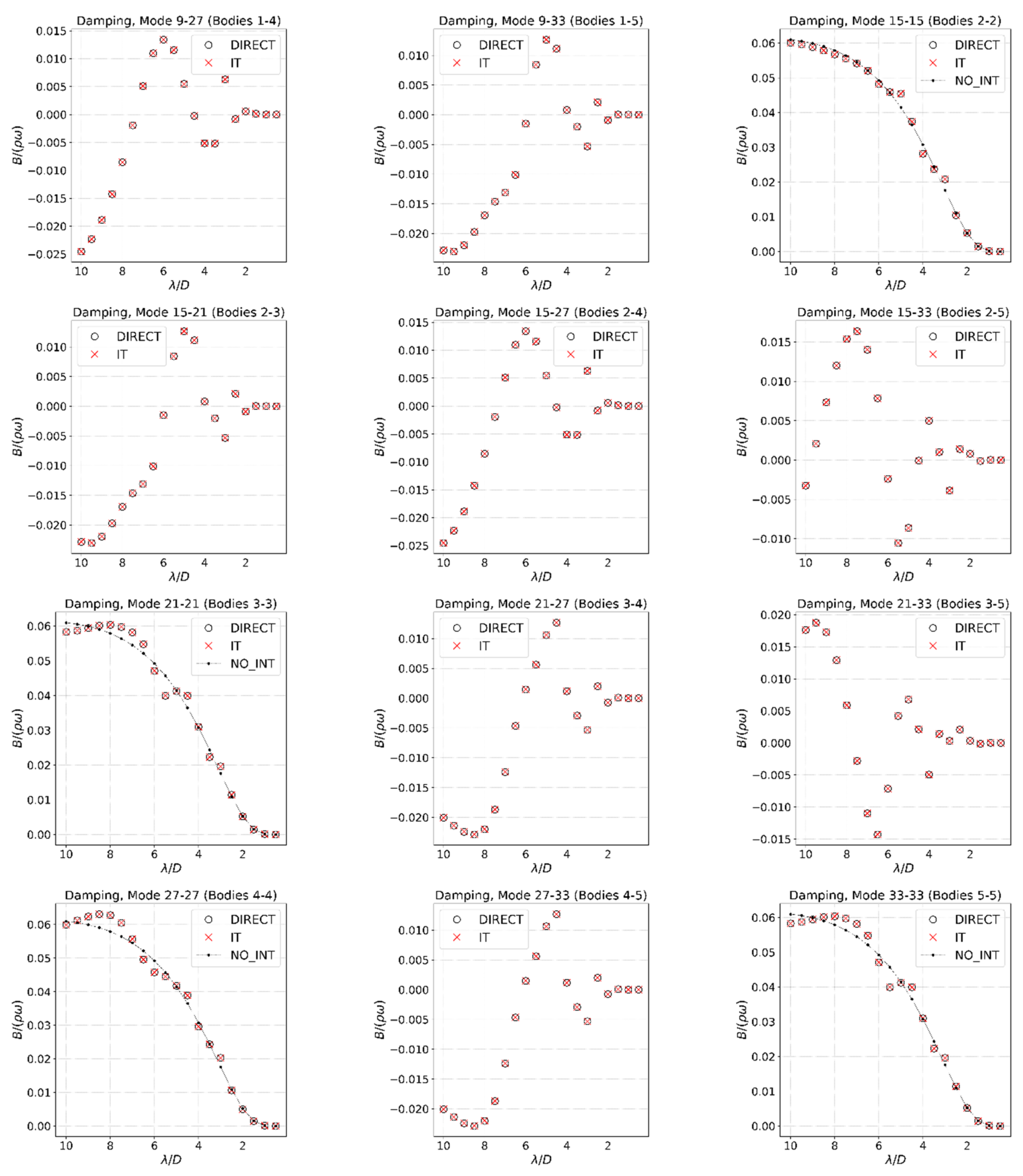
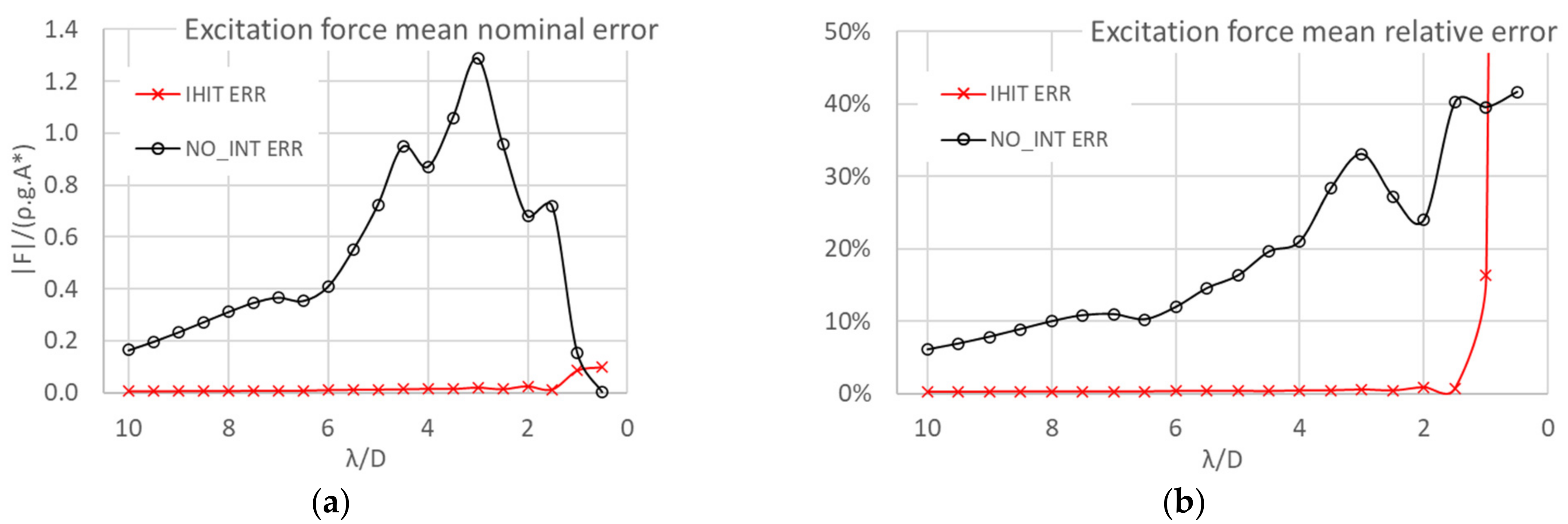
3.1. Verification

Consider the multi-body problem consisting of five identical bodies, each one free to oscillate only in heave (see Figure 1a). Each body is a cylinder with diameter $D$ and draft $T=D/2$. The bottom is flat and the water depth $h=20T=10D$. The bodies’ positions are symmetric about the $x$ axis.

One wishes to attain the added mass and damping matrices as well as the excitation forces on the array including the interaction effects considering different undisturbed wave conditions (amplitude, period, heading, and phase) on each body. One cannot arbitrarily introduce different incoming waves on different points in WAMIT’s Equation (8) for the diffraction problem, but Equation (9) can be used by making one or more bodies act as (numerical) wave generators. In Figure 1a, body W₁ is a small cylindrical body forced-oscillating with unit amplitude in heave at an angular frequency $\omega$. This body’s geometry is a 1/8 scaled down version of the remaining bodies. Note that Figure 1a represents a view from above and that the relative sizes of bodies 1 through 5 and W₁ are in scale.

Consider the set of $N$ problems where ${\omega }_j^2=g\frac{2\pi }{{\lambda }_j}\tanh \left(\frac{2\pi }{{\lambda }_j}h\right)\left(rad/s\right),j=1,\dots ,N_{\omega }$, with ${\lambda }_j/D$ as given in

Table 1. Undisturbed incoming wave conditions for oscillating body W₁ at each body.

λ/D	${\mathit{A}}_1$	${\mathit{\epsilon }}_1$	${\mathit{\beta }}_1$	${\mathit{A}}_2/{\mathit{A}}_1$	${\mathit{\epsilon }}_2$	${\mathit{\beta }}_2$	${\mathit{A}}_3/{\mathit{A}}_1$	${\mathit{\epsilon }}_3$	${\mathit{\beta }}_3$	${\mathit{A}}_4/{\mathit{A}}_1$	${\mathit{\epsilon }}_4$	${\mathit{\beta }}_4$	${\mathit{A}}_5/{\mathit{A}}_1$	${\mathit{\epsilon }}_5$	${\mathit{\beta }}_5$
	m	deg	deg	-	deg	deg	-	deg	deg	-	deg	deg	-	deg	deg
0.5	1.67 × 10−2	49.73	18	0.922	112.33	36	0.767	–52.89	36	0.786	–119.88	18	0.852	–23.37	0
1.0	1.14 × 10−2	–0.68	18	0.922	30.61	36	0.767	127.98	36	0.786	94.49	18	0.852	–37.25	0
1.5	7.83 × 10−3	–136.46	18	0.922	124.38	36	0.767	–170.73	36	0.786	46.95	18	0.852	–40.87	0
2.0	5.72 × 10−3	155.96	18	0.922	171.58	36	0.767	–139.77	36	0.786	23.48	18	0.852	137.63	0
2.5	4.39 × 10−3	–172.44	18	0.922	–87.95	36	0.767	166.94	36	0.786	–62.45	18	0.853	–43.12	0
3.0	3.50 × 10−3	88.70	18	0.922	–140.89	36	0.767	–108.51	36	0.786	0.33	18	0.852	–43.55	0
3.5	2.88 × 10−3	–84.68	18	0.922	78.47	36	0.767	–150.93	36	0.786	–57.63	18	0.852	–146.66	0
4.0	2.42 × 10−3	55.26	18	0.922	–116.94	36	0.767	87.28	36	0.786	168.92	18	0.852	46.02	0
4.5	2.06 × 10−3	164.16	18	0.923	11.06	36	0.767	–87.41	36	0.787	–14.85	18	0.853	–164.07	0
5.0	1.79 × 10−3	–108.65	18	0.922	113.47	36	0.767	60.83	36	0.786	126.14	18	0.853	–44.13	0
5.5	1.57 × 10−3	–37.35	18	0.921	–162.67	36	0.766	–177.85	36	0.786	–118.46	18	0.852	53.98	0
6.0	1.40 × 10−3	22.03	18	0.921	–92.78	36	0.766	–76.74	36	0.786	–22.31	18	0.851	135.77	0
6.5	1.25 × 10−3	72.29	18	0.923	–33.66	36	0.767	8.80	36	0.786	59.04	18	0.852	–154.97	0
7.0	1.13 × 10−3	115.41	18	0.924	16.98	36	0.768	82.13	36	0.787	128.79	18	0.853	–95.60	0
7.5	1.02 × 10−3	152.83	18	0.925	60.87	36	0.768	145.70	36	0.787	–170.72	18	0.855	-44.18	0
8.0	9.32 × 10−4	–174.39	18	0.924	99.30	36	0.768	–158.65	36	0.788	–117.79	18	0.855	0.80	0
8.5	8.55 × 10−4	–145.44	18	0.923	133.25	36	0.769	–109.54	36	0.788	–71.09	18	0.855	40.48	0
9.0	7.89 × 10−4	–119.71	18	0.922	163.46	36	0.769	–65.89	36	0.788	–29.60	18	0.854	75.77	0
9.5	7.31 × 10−4	–96.68	18	0.921	–169.49	36	0.768	–26.86	36	0.788	7.51	18	0.853	107.36	0
10.0	6.80 × 10−4	–75.98	18	0.920	–145.12	36	0.767	8.26	36	0.787	40.91	18	0.851	135.82	0

A_j, β_j and ε_j,(i = 1,…,5) stand for wave amplitude, heading angle, and phase angle at the jth body, respectively.

.

The resulting radiated wave patterns (real part of the wave elevation) for selected oscillation frequencies of W₁ are shown in Figure 2.

From visual observation, it is seen that the waves can be considered locally planar at a short distance from each body. Similar plots but where scattering due to presence of the other bodies is included are shown in Figure 3, where it is clear that the wave field is considerably disturbed within the wave frequency range studied, exhibiting significant array scattering phenomena.

In Table 1, the prescribed incoming undisturbed wave conditions at each body center location are listed for each forced-oscillating body frequency. In each, the amplitude of the waves $A_1$ and phases are relative to the motion of $W_1$. The amplitudes could have been normalized as suggested in Section 2.5 (step 3). However, these were left unchanged to deliberately have very small amplitudes of the incoming waves to verify possible numerical truncation errors within the implementation of the algebraic procedure in the interaction theory.

The values in Table 1 were obtained by running a simulation in WAMIT for the radiation problem of body $W_1$ oscillating in heave. The incoming undisturbed wave amplitudes at the points corresponding to the center of each body were extracted from WAMIT’s output and considered as local long-crested incident plane waves with headings as given in Figure 1a. Table 1 is the input to the inhomogeneous interaction procedure described in Section 2.5 (step 3). The mesh of each body and its panel distribution are presented in Figure 1b. The panel length is about 0.26 λ for the shortest wavelength considered. Therefore, the results for these high frequencies may not be accurate, but its relevance is negligible considering the focus of the present study.

The control surface surrounding the body, for performing steps 6 and 7 in Section 2.5, was the submerged surface of a truncated cylinder with radius 0.55 D extending from $z=0$ to $z=-h$. The surface is discretized with $N_z\times N_{\theta }$ panels, where $N_z=200$ is the number of points in the vertical direction and $N_{\theta }=2\times {10}^8$ is the number of points in the angular direction. Cosine spacing in the vertical direction was applied. The body mesh, mass characteristics, and water depth were kept the same as for the cylinder case in [19].

The results obtained are shown in Figure 4, Figure 5, Figure 6 and Figure 7. These correspond to the excitation forces’ real and imaginary components, the added mass, and the radiation damping, respectively.

The verification was clearly accomplished by observing Figure 4, Figure 5, Figure 6 and Figure 7, with all quantities showing excellent agreement between the interaction theory and the direct method. As a reference, the quantities relative to the bodies in isolation are also presented and demonstrate the need for properly accounting for both the diffraction under inhomogeneous wave conditions and radiation interaction within the frequency range considered. Naturally, the interactions become less important for very short waves, and wave scattering itself becomes negligible for very long waves. Both these assertions are straightforwardly verified in Figure 4, Figure 5, Figure 6 and Figure 7.

An overall nominal and relative error quantification is presented in Figure 8 for the excitation forces considering the interaction theory and the bodies in isolation. The values shown are averages, but the error variation between the different bodies is marginal, meaning that the plots are good indicators of the errors. In Figure 8a, one can see that the nominal error of the interaction theory is close to zero except for the two shortest wavelengths. The corresponding relative mean errors are, respectively, 16.3% and 748% for the two highest frequencies, which compares to 39.6% and 41.67% when neglecting interactions. The reason for this error amplification could be due to numerical truncation errors. Specifically, when using the interaction theory with input from WAMIT, which has only single precision, when the excitation forces, and the quantities from which they are derived from, become very small, as is the case for these two frequencies. Another possible explanation is that the consideration of local incoming undisturbed planar waves hitting each body loses its validity for wavelengths closer to the body diameter, and the circular crests cannot be neglected. One should realize that, in both cases, the source of the error is not related to the interaction theory.

Irrespective of the origin of the error amplification, it is important to bear in mind that for wavelengths of this order (or shorter), the diffraction forces are close to zero and the radiation couplings between the bodies are likewise negligible (see Figure 4, Figure 5, Figure 6 and Figure 7). Therefore, one can use the procedure herein described, deeming the verification excellent for practical cases. Here, it is worth to note that for the other frequencies studied, the error typically increased from about 0.1% to a maximum of 0.9% as the frequency increased, while the isolated body approximation had errors in the range of about 10–40% (see Figure 8b). It is also worth mentioning that it is always possible to simply use the no-interaction approach for wavelengths outside the range where multi-body interaction is significant.

3.2. Frequency Inhomogeneity in a WEC Farm

It is important to realize that even in the (unrealistic) case of the model used in Section 3.1 for verification, WAMIT cannot consider frequency inhomogeneity.

Consider the case of a wave farm deployed in a location where local conditions force short waves to break and dissipate in some areas, effectively acting as a low-pass filter in sections of the array. This situation is easily considered using the procedure presented herein. Using the same model of Section 3.1 for illustration purposes, one can simply remove the higher half of the incoming undisturbed wave frequency (λ/D < 6) components for bodies 1 and 4, deemed as WECs in a wave farm to impose such a condition.

In Figure 9, the motions of each body are plotted for the case similar to Section 3.1 and the one where the local frequency truncations have been applied to the incoming undisturbed waves with no Power Take Off (PTO) or viscous damping applied.

Likewise, the absorbed power in both configurations is shown in Figure 10, where a PTO damping equal to each body’s radiation damping at λ/D = 5.0 is applied.

Figure 9 is more interesting for the general case of multi-body interaction, while Figure 10 is more relevant for wave farms. In both figures, results pertaining to bodies 1 and 4 for the lower half of the frequency range are the response of the bodies solely due to the excitation forces originating from the scattering of the incoming undisturbed wave system in the other bodies, but where the presence of all bodies is considered for diffraction computation, plus the ones arising from the multi-body radiation. As expected, the results show that there are motions and absorbed power beyond the undisturbed incoming local wave system frequency range at these bodies.

It is interesting, although not surprising, to see how the absence of high frequency waves in bodies 1 and 4 led to amplification of motions and power iwo the resonant frequency for bodies 3 and 5, showing a destructive interaction that is no longer there. In fact, the difference between the sum of the product of squares of undisturbed wave amplitudes with frequency of undisturbed incoming waves between both cases shows a reduction of 43% in what can colloquially be defined as a measure of the total available wave power, whereas the power absorption is reduced by only 21%. Naturally, these assessments are but illustrative of the interaction phenomena, as the wave field and the characteristics of the wave farm used herein are not deemed to be of a real wave farm design.

4. Discussion

In the present study, it was shown that the interaction theory originally presented in [12], and modified in [19] to allow the use of standard diffraction codes for solving the linear potential, can also be used when accounting for inhomogeneous sea states across the domain of a multi-body problem without modifying its fundamental supporting algebraic relations. A procedure to include the inhomogeneous sea state in the implementation of the theory was presented, which avoids the need to modify the inner core functions of the code available in [29] considerably.

The new procedure should allow researchers to accurately include wave field inhomogeneity in numerical models of wave farms and accurately assess the sensitivity of the results to the perturbations on otherwise perfectly coherent long-crested wave components. These perturbations are realistic and will significantly influence the results of many published studies concerning optimal wave farm layout and wave farm power output in general, which, to the best of the author’s knowledge, have not considered such perturbations. In this respect, one should bear in mind that coastal or nearshore structures are more prone to be hit by inhomogeneous wave fields arising from shore reflections and bathymetric variations. Furthermore, near-shore wave climates tend to exhibit shorter peak periods, therefore exhibiting a relative higher energy for waves within the wavelength range where interaction effects are non-negligible.

Additionally, dangerous modes of operation including wave-trapping modes are dependent on the direction, frequency, and amplitude distribution at each body composing the structure or array of bodies. For the specific case of VLFSs such as floating bridges or wave farms composed of WECs connected through a structure, there is a need to properly account for inhomogeneity and interaction among floating elements, which can possibly excite natural flexural modes that are otherwise neglected if full diffraction interaction is not accounted for.

The focus of the present paper is to demonstrate the capability of the interaction theory to cope with inhomogeneous wave conditions and the results are shown only for regular waves. However, the generalization to irregular waves is straightforward and can be implemented following the steps listed in Section 2.5.

It is also worth noticing that the absence of the consideration of evanescent wave modes in the present theory did not show any effect on the results for the frequency range where multi-body interactions are non-negligible.

Regarding future work, perhaps the most interesting immediate step would be to include the output regarding mean second order drift forces. Work on delineating a possible strategy has been initiated by the author, with the considerable increase in complexity being the biggest challenge.

References

- Rodrigues, J.M.; Økland, O.; Fonseca, N.; Leira, B.; Alsos, H.S.; Abrahamsen, B.C.; Aksnes, V.; Lie, H. Design and verification of large floating coastal structures: Floating bridges for fjord crossings. In Proceedings of the Thirtieth International Ocean and Polar Engineering Conference, Shanghai, China, 11–16 October 2020. [Google Scholar]
- Fonseca, N.; Chi, Z.; Rodrigues, J.M.; Ren, N.X.; Hellan, O.; Magee, A.R. Hydrodynamic model tests with a large floating hydrocarbon storage facility. In Proceedings of the ASME 38th International Conference on Ocean, Offshore and Arctic Engineering, Glasgow, Scotland, 9–14 June 2019; Volume 6. [Google Scholar]
- Kagemoto, H.; Fujino, M.; Murai, M. Theoretical and experimental predictions of the hydroelastic response of a very large floating structure in waves. Appl. Ocean Res. 1998, 20, 135–144. [Google Scholar] [CrossRef]
- Kagemoto, H.; Yue, D.K.P. Hydrodynamic interaction analyses of very large floating structures. Mar. Struct. 1993, 6, 295–322. [Google Scholar] [CrossRef]
- Folley, M.; Whittaker, T.J.T. The effect of sub-optimal control and the spectral wave climate on the performance of wave energy converter arrays. Appl. Ocean Res. 2009, 31, 260–266. [Google Scholar] [CrossRef]
- Fitzgerald, C.; Thomas, G. A preliminary study on the optimal formation of an array of wave power devices. In Proceedings of the 7th European Wave and Tidal Energy Conference, Porto, Portugal, 11–13 September 2007. [Google Scholar]
- WAMIT INC. Wamit User Manual, v7.4.; WAMIT INC: Chestnut Hill, MA, USA, 2020. [Google Scholar]
- Babarit, A.; Delhommeau, G. Theoretical and numerical aspects of the open source bem solver nemoh. In Proceedings of the 11th European Wave and Tidal Energy Conference (EWTEC2015), Nantes, France, 6–11 September 2015. [Google Scholar]
- BUREAU VERITAS. 2021. Available online: https://marine-offshore.Bureauveritas.Com/hydrostar-software-powerful-hydrodynamic (accessed on 20 March 2021).
- SINTEF OCEAN. 2019. Available online: https://www.Sintef.No/globalassets/sintef-ocean/factsheets/muldif.Pdf (accessed on 20 March 2021).
- SINTEF OCEAN. 2021. Available online: https://www.Sintef.No/en/software/sima/ (accessed on 20 March 2021).
- Kagemoto, H.; Yue, D.K.P. Interactions among multiple three-dimensional bodies in water waves: An exact algebraic method. J. Fluid Mech. 1986, 166, 189–209. [Google Scholar] [CrossRef]
- Yilmaz, O.; Incecik, A. Analytical solutions of the diffraction problem of a group of truncated vertical cylinders. Ocean Eng. 1998, 25, 385–394. [Google Scholar] [CrossRef]
- Linton, C.M.; McIver, P. Handbook of Mathematical Techniques for Wave/Structure Interactions; Chapman & Hall/CRC: Boca Raton, FL, USA, 2001; p. 304. [Google Scholar]
- Child, B.F.M.; Venugopal, V. Optimal configurations of wave energy device arrays. Ocean Eng. 2010, 37, 1402–1417. [Google Scholar] [CrossRef]
- Yoshida, K.; Goo, J.-S. A numerical method for huge semisubmersible responses in waves. Trans. Soc. Naval Archit. Mar. Eng. 1990, 98, 365–387. [Google Scholar]
- Chakrabarti, S. Hydrodynamic interaction forces on multi-moduled structures. Ocean Eng. 2000, 27, 1037–1063. [Google Scholar] [CrossRef]
- McNatt, J.C.; Venugopal, V.; Forehand, D. The cylindrical wave field of wave energy converters. Int. J. Mar. Energy 2013, 3, e26–e39. [Google Scholar] [CrossRef]
- McNatt, J.C.; Venugopal, V.; Forehand, D. A novel method for deriving the diffraction transfer matrix and its application to multi-body interactions in water waves. Ocean Eng. 2015, 94, 173–185. [Google Scholar] [CrossRef] [Green Version]
- Flavia, F.F.; McNatt, C.; Rongere, F.; Babarit, A.; Clement, A.H. A numerical tool for the frequency domain simulation of large arrays of identical floating bodies in waves. Ocean Eng. 2018, 148, 299–311. [Google Scholar] [CrossRef] [Green Version]
- McNatt, J.C.; Porter, A.; Chartrand, C.; Roberts, J. The performance of a spectral wave model at predicting wave farm impacts. Energies 2020, 13, 5728. [Google Scholar] [CrossRef]
- Leira, B.J.; Dai, J. Extreme dynamic response of extended bridge structures subjected to inhomogeneous environmental loading. In Proceedings of the EURODYN 2020 XI International Conference on Structural Dynamics, Athens, Greece, 23–16 November 2020. [Google Scholar]
- Fonseca, N.; Bachynski, E.E. LFCS Review Report—Environmental Loads Methods for the Estimation of Loads on Large Floating Bridges; SINTEF Ocean: Trondheim, Norway, 2018. [Google Scholar]
- Cheng, Z.S.; Gao, Z.; Moan, T. Wave load effect analysis of a floating bridge in a fjord considering inhomogeneous wave conditions. Eng. Struct. 2018, 163, 197–214. [Google Scholar] [CrossRef]
- Xiang, X.; Viuff, T.; Leira, B.; Oiseth, O. Impact of hydrodynamic interaction between pontoons on global responses of a long floating bridge under wind waves. In Proceedings of the ASME 37th International Conference on Ocean, Offshore and Arctic Engineering, Madrid, Spain, 17–22 June 2018; Volume 7a. [Google Scholar]
- Belibassakis, K.; Bonovas, M.; Rusu, E. A novel method for estimating wave energy converter performance in variable bathymetry regions and applications. Energies 2018, 11, 2092. [Google Scholar] [CrossRef] [Green Version]
- Dai, J.; Leira, B.J.; Moan, T.; Kvittem, M.I. Inhomogeneous wave load effects on a long, straight and side-anchored floating pontoon bridge. Mar. Struct. 2020, 72, 102763. [Google Scholar] [CrossRef]
- Abramowitz, M.; Stegun, I.A. Handbook of Mathematical Functions with Formulas, Graphs, and Mathematical Tables; U.S. Department of Commerce: Washington, DC, USA, 1964; 1046p.
- McNatt, C. Mwave. 2014. Available online: https://github.com/cmcnatt/mwave (accessed on 20 March 2021).