Modelling of a Flow-Induced Oscillation, Two-Cylinder, Hydrokinetic Energy Converter Based on Experimental Data

Abstract

The VIVACE Converter consists of cylindrical oscillators in tandem subjected to transverse flow-induced oscillations (FIOs) that can be improved by varying the system parameters for a given in-flow velocity: damping, stiffness, and in-flow center-to-center spacing. Compared to a single isolated cylinder, tandem cylinders can harness more hydrokinetic energy due to synergy in FIO. Experimental and numerical methods have been utilized to analyze the FIO and energy harnessing of VIVACE. A surrogate-based model of two tandem cylinders is developed to predict the power harvesting and corresponding efficiency by introducing a backpropagation neural network. It is then utilized to reduce excessive experimental or computational testing. The effects of spacing, damping, and stiffness on harvested power and efficiency of the established prediction-model are analyzed. At each selected flow velocity, optimization results of power harvesting using the prediction-model are calculated under different combinations of damping and stiffness. The main conclusions are: (1) The surrogate model, built on extensive experimental data for tandem cylinders, can predict the cylinder oscillatory response accurately. (2) Increasing the damping ratio range from 0–0.24 to 0–0.30 is beneficial for improving power efficiency, but has no significant effect on power harvesting. (3) In galloping, a spacing ratio of 1.57 has the highest optimal harnessed power and efficiency compared with other spacing values. (4) Two tandem cylinders can harness 2.01–4.67 times the optimal power of an isolated cylinder. In addition, the former can achieve 1.46–4.01 times the efficiency of the latter. (5) The surrogate model is an efficient predictive tool defining parameters of the Converter for improved energy acquisition.

1. Introduction

The present trend towards clean renewable energy is very strong [1,2,3]. It is gaining momentum worldwide and it is unlikely to slow down despite the current low cost of fossil fuels. Consequently, the exploration and development of renewable energy sources are urgent. Marine energy, as a widely distributed sustainable energy source, with the characteristics of strong stability and predictability, and high-energy density, has been studied by a considerable number of scholars [4,5,6]. One of the major forms of marine energy is horizontal hydrokinetic energy in ocean currents, tides, and rivers [7]. In last decade, research on the utilization of ocean current energy for power generation is widespread [8,9], with the main power generation device being the underwater turbine [10,11]. Underwater turbines, which generate electricity by rotation of their impeller induced by the incoming flow, require a high flow velocity (2.0–2.5 m/s) to start. At most sea locations, however, the current velocity is low, with an average velocity of about 0.4–1.5 m/s and a maximum velocity generally not exceeding 2.5 m/s. Typical river flows are 1.0–1.5 m/s.

When current flows past a bluff elongated structure, the shed vortices formed behind the structure apply alternating forces which may induce vibration of the structure, in the form of nonlinear resonance called vortex-induced vibration (VIV) [12,13,14]. In addition to causing structural damage, VIV has been utilized for energy harvesting on account of the reason that it can be induced even than the ocean current is lower than 0.1 m/s [15]. In 2006, a new energy device named the Vortex-Induced Vibration for Aquatic Clean Energy (VIVACE) Converter, has been proposed by the team of Bernitsas at the University of Michigan [16]. VIVACE uses the flow-induced oscillation (i.e., VIV and galloping) of one or more cylindrical oscillators to convert the hydrokinetic energy to the electrical energy. Crucially, the FIO of rigid cylinders is driven by transverse alternating lift and results in oscillatory FIO motion [17]. Alternating lift technologies (ALT) [2,18], imitating the natural motion of fish, provides an environmentally compatible way of harnessing energy from the flow as low as 0.274 m/s [19,20], realizing the energy harvesting from low flow rate.

Since 2006, the VIVACE Converter has been continuously innovated and improved including extending the power generation nature of oscillation from vortex-induced vibration [21] to galloping [22] with high energy acquisition, high amplitude, and low vibration frequency. Additionally, the number of oscillators increased from a single isolated cylinder [22] to multiple cylinders [23]. The oscillator features have been extended from linear [24] to nonlinear [18]. So far, the two-cylinder VIVACE Converter has a maximum capture efficiency of 69% in lab setting [25]. It is noteworthy that the above improvements are based on a large number of experimental tests [23,26], and numerical simulations [24,27,28] conducted in the Marine Renewable Energy Laboratory (MRELab) at the University of Michigan, Ann Arbor, U.S. It took a decade for experiments to be carried out and continuously improve the Converter performance. Such experiments require expensive equipment and human resources [29]. Besides that, the correctness of numerical simulation is dependent on the selection of simulation methods. At high Reynolds number, the accuracy of numerical simulation is greatly reduced. In order to circumvent the problems inherent in experimental and numerical simulations, a modeling method named “surrogate model” has been widely used by researchers in recent years [30,31]. This surrogate model also can be considered as an effective substitute for experimental device and numerical software to predict the data for cases that have not be directly measured. Based on its modeling efficiency, predictive strength, and ability to explore unknown data, surrogate models have been utilized in many engineering fields [29,30,32,33,34].

Surrogate-based models can be constructed correctly by utilizing the corresponding predictive method. Several predictive approaches, such as polynomial regression [29], kriging model [33] and artificial neural network [35], have been used to establish a surrogate model for accurate prediction. Nevertheless, some published studies illustrate that the polynomial modeling has low accuracy for highly nonlinear cases [29,33]. Additionally, the Kriging model has relatively complex structure and is more difficult to build because it requires determining the maximum possible estimator and assuming the global function form [33]. Artificial neural network methods, such as back propagation neural network (BPNN) and the radial basis function neural network (RBFNN) method, have been widely used because they can effectively deal with nonlinear forecasting problems [35,36,37]. In 2018, Wu et al. established a model of VIVACE Converter with an isolated single cylinder by introducing the radial basis function neural network method based on the “Isight 5.0” (an integration platform for a simulation-based design process) [33]. This model can reasonably predict the effects of flow velocity, spring stiffness, and damping ratio on the harnessed power and corresponding efficiency [33]. In the case of a converter with multiple cylinders in tandem, the interaction of the cylinders generates more power and at higher efficiency. This has been proven in the lab [23,25] and tested in field-tests [38]. However, modeling of a FIO Converter with multiple oscillators has not been conducted before. Sun et al. showed that the VIVACE Converter with two tandem cylinders is conducive to improve the performance of power harvesting compared with a single oscillator converter [23]. This is the motivation to pursue modeling of a double cylinder converter in this paper. In [33], the relationship of influencing factors and power have not been directly built, but it is solved by the second-order linear differential equation and power equation [33], meaning that the probability of errors will increase. Therefore, this paper used the programming software to write neural networks instead of the “Isight 5.0”, and directly searched for the relationship between input variables and power. The BPNN and RBFNN both can build the nonlinear relationship between input variables and power. However, the structure of BPNN is simpler than that of RBFNN when solving the problems with the same precision requirements. Moreover, the number of hidden layer neurons of RBF neural network is much higher than that of BPNN when there are more training samples, which makes the complexity and computation of RBFNN increase greatly. Based on above two reasons, we selected the BPNN to establish the surrogate model of VIVACE Converter with two tandem cylinders.

In this paper, four different surrogate-based models, three for two tandem cylinders with different spacing and one for an isolated single cylinder are established by implementing the back propagation neural network method. This modeling implementation is based on sample training and testing of the experimental data. Based on the established surrogate model of the VIVACE Converter, this paper explores and analyzes the influences of harnessing damping ratio, spring stiffness, and spacing ratio on the harnessed power and the corresponding efficiency of the VIVACE Converter. Extending the selected range of harnessing damping ratio and spring stiffness is conducive to enhancing the oscillating responses, especially for the power efficiency. In addition, a tandem cylinder with reasonable combinations of various input parameters can harness more power at higher efficiency than that of the isolated single-cylinder due to the positive synergy between cylinders in close proximity.

2. Physical Model and Mathematical Model

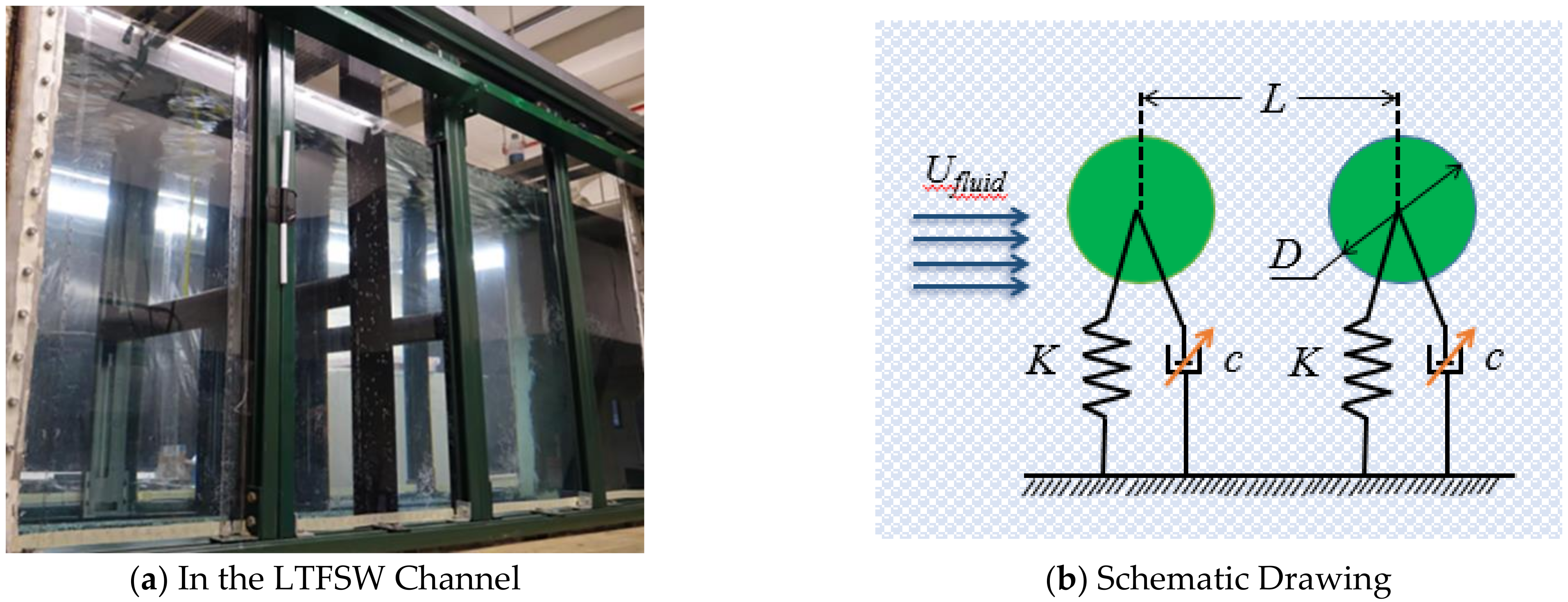
2.1. Experimental Facility: LTFSW Channel

All tests were conducted in the Low Turbulence Free Surface Water (LTFSW) Channel in the MRELab of the University of Michigan. In the LTFSW Channel, 10,000 gallons (37,854 lt) of freshwater are recirculated at speed up to 1.5 m/s realized by using an impeller powered by a 20 hp induction motor. The test section is 2.44 m long and 1.0 m wide and is made of transparent plexiglass, which allows for visualization of both cylinders in FIO using argon lasers of 5 W and adding aluminum oxide particles of 100 μm. Figure 1 shows the VIVACE Converter with a two cylinder-oscillator system in the Channel. The water depth of the test section is 1.17 m and the maximum flow velocity is kept lower than 1.35 m/s to prevent damage due to the galloping instability.

2.2. Cylinders with Distributed Roughness

Passive turbulence control (PTC) [23] consists of two roughness strips on the surface of the smooth cylinder. It was introduced in the VIVACE Converter and extensively studied in the MRELab [19,20,24,27] in order to harvest more marine hydrokinetic energy from the steady flow using FIO of cylinders. As shown in Figure 2, the total height of the PTC consists of double-sided tape at the bottom, sandpaper in the middle, and coarse sand on top. In addition, the total height of PTC is set to be about equal to the boundary layer thickness of the fluid around the cylinder. Attaching the PTC on the surface of the cylinder results in geometric asymmetry of the cross-section of the oscillator inducing the galloping, which is characterized by unstable oscillation and high energy acquisition. A secondary benefit is that PTC fixes the separation point in VIV, which for a smooth cylinder oscillates by about 5° to 10°. This seemingly minute detail is very important and difficult to predict numerically. A negative effect of PTC is that the surface roughness reduces the vortex strength in VIV and the response amplitude. This is corrected by introducing smooth PTC in the form of step surface elements like simple tape.

2.3. Vck System

Physical springs and dampers were applied to the early VIVACE Converter models in the MRELab. For systematic experiments, however, to test different combinations of spring stiffness and damping ratio, replacing the physical springs and dampers requires extensive design, fabrication, calibration, and alignment time. Besides that, the nonlinear viscous damping of a Converter is not easily modeled by a physical damper. To compensate for the above two challenges, the virtual spring-damping (Vck) system was developed and improved by the MRELab and was used to emulate physical springs and dampers. In 2011, Lee et al. [26] developed the first generation of Vck. In 2013, Sun et al. [39] developed the embedded second-generation Vck system, which reduced the controller response time by three orders of magnitude by eliminating LabView. It used digital instead of analogue signal and the damping model simplified significantly. The Vck system is a controller with a feedback loop that uses a servo motor encoder to track the position and speed of the cylindrical oscillator and to provide the necessary torque to simulate spring stiffness, as well as the required linear viscous damping. Further, it can emulate any nonlinear spring and damper function and its parametric values.

2.4. Mathematical Model of Harnessed Power and Harnessing Efficiency

To reasonably and systematically analyze the performance of the VIVACE Converter, the harnessed power P_harness and harnessed efficiency η_harness are proposed and introduced as two important evaluation metrics. As expressed in Equation (1), the harnessed power is positively correlated with the oscillating system mass, harnessing damping ratio ζ_harness, and natural frequency of oscillator in water f_n,water, respectively. A detailed description of ζ_harness and f_n,water is provided in [23].

$$P_{harness}=8{\mathit{\pi }}^3{m}_{sys}{\zeta }_{harness}{\left(A{f}_{osc}\right)}^2{f}_{n,water}$$

(1)

where A and f_osc are, respectively, the oscillating amplitude and frequency of the cylinder. The harnessed power can be calculated by averaging the instantaneous harnessed power. For a linear system, since Equation (1) depends explicitly on the oscillating mass of the system, m_sys, power can be calculated via the recorded amplitude and the frequency of oscillation. For either linear or nonlinear damping, the instantaneous power can be written as follows:

$$P_{harness}\left(t\right)=c_{harness}{\dot{y}}^2\left(t\right)$$

(2)

where $\dot{y}\left(t\right)$ is the oscillation speed of the cylinder as measured by the Vck system. Equation (2) does not depend on the specific way the added mass is calculated or even the value of the added mass explicitly; it cancels out, thus, eliminating the need to deal with modeling of the added mass [13].

The power of fluid-flow can be calculated as:

$$P_{Fluid}=\frac{1}{2}\rho U^3\left(2A_{\max }+D\right)L$$

(3)

where A_max represents the maximum amplitude, ρ is the fluid density, U is the incoming flow velocity, and D and L are the diameter and length of the cylinder, respectively. The Betz Limit is the theoretical maximum efficiency of power extracted from the flowing fluid. Therefore, the converter efficiency can be defined as:

$${\eta }_{harness}=\frac{P_{harness}}{P_{Fluid}\times BetzLimit}\times 100\%$$

(4)

3. Modeling of the Converter

In this section, four different surrogate models of the VIVACE Converter are established based on the BP neural network method by using the experimental data measured for flow velocity, spring stiffness, and harnessing damping ratio values uniformly distributed within the specified range [23,35]. These four models correspond to the isolated single-cylinder device and three double-cylinder devices with tandem spacing ratios of L/D = 1.57, 2.00, and 2.57. The surrogate models built in this section can construct the complex nonlinear mathematical relationship between input variables (U, spring stiffness K and ζ_harness) and objective variable (P_harness or η_harness). After the establishment of the prediction model, the power harvesting of the VIVACE Converter can be predicted by inputting appropriate and reasonable values of the input variables, which are not limited to the tested experimental data. The principle of BP neural network is described in Section 3.1. The construction and validation of surrogate models are presented in Section 3.2.

3.1. Principle of BP Neural Network

The BP neural network is a multi-layer feedforward network trained by an error inverse propagation algorithm. It is one of the most widely used neural network models [36,37]. As illustrated in Figure 3, a BP neural network is mainly composed of the input layer, middle layer, and output layer. The middle structure can be designed as single layer or multiple hidden layers. The node numbers of the neural network of the above three layers is set as p (1 ≤ i ≤ p), s (1 ≤ j ≤ s), r (1 ≤ k ≤ r), respectively. The neurons between the adjacent layers are connected in the form of weights and biases. In addition, the weights or biases of the input layer to the hidden layer and the hidden layer to the output layer are, respectively, w_ij and w_jk or a_j and b_k.

The BP neural network method consists of the forward-propagation of input signal and back-propagation of error. For the forward-propagation of the input signal, the neurons of the input layer receive the input signal x_i and transmit it to the neurons of the hidden layer. The hidden layer is the internal information processing layer and is responsible for information transformation. The output signal G_j of the hidden layer can be expressed as in Equation (5):

$$G_j=f\left({\displaystyle \sum }_{i=1}^p{w}_{ij}{x}_i+a_j\right)$$

(5)

where f is the nonlinear transfer function, also called the activation function. Then, the hidden layer transmits the signal G_j to the output layer. The output layer completes the signal processing and outputs it. The output signal Q_k is calculated by the Equation (6) as follows:

$$Q_k={\displaystyle \sum }_{j=1}^s{G}_j{w}_{jk}+b_k$$

(6)

The error E that exists between the expected output D_k (i.e., experimental data) and predicted output Q_k can be expressed as follows:

$$E=\frac{1}{2}{\displaystyle \sum }_{k=1}^r{\left(D_k-Q_k\right)}^2$$

(7)

In the process of the back-propagation, the error will continuously correct the network connection weights and biases of two adjacent layers by backward propagation along with the output layer, hidden layer, and input layer, respectively. The process will be completed when the output error E satisfies the step requirement or reaches the maximum training time of the neural network.

3.2. Construction and Validation of Surrogate Model

The correctness of the construction of the surrogate model is largely determined by the selection of input parameters. For the VIVACE Converter, the most easily changeable variable parameters are the incoming flow velocity, harnessing damping ratio, and spring stiffness, which would directly affect the acquisition of harnessed power and the formation of power efficiency. Due to the reason that there are only three groups of optional spacing ratios, the spacing ratio (L/D = 1.57, 2.00, 2.75) is not included in the input variables. In addition, the output objective is harnessed power measured experimentally in reference [23]. The modeling of power efficiency can be realized by utilizing the same approach as used for the power harvesting model. Nevertheless, in the following discussion, only the surrogate model of harnessed power is considered. The steps for the construction and validation of the surrogate model in order of occurrence are: determination of neural network structure, sample training, and sample testing.

3.2.1. Range of Input Variables

The selection range of input experimental design parameters is constrained by the geometry of the model converter (Figure 1), engineering applications, and mechanical properties of cylinder oscillators.

Incoming flow velocity (U): The incoming flow velocity is selected in the range from 0.39 to 1.31 m/s with an interval of 0.04 m/s, which covers to the actual ocean conditions of water current [40] and the experimental condition of Sun et al. [23,35].

Harnessing damping ratio (ζ_harness): In order to trigger FIO easier in VIV branches and harvest higher power in galloping, the values of ζ_harness chosen vary from 0.00 to 0.24 in intervals of 0.04.

Spring stiffness (K): The five spring stiffness values are evenly chosen from 400 N/m to 1200 N/m in increments of 200 N/m. Low stiffness with low damping induce high oscillating amplitude, resulting in reaching the amplitude limit of the water channel. Further, the highest value of K is chosen depending on the strength limit of the timing belts of the Vck controller system. The input experiment-design parameters and its constraint range for four different surrogate models are uniform and summarized in

Table 1. Values of experimental design variables (U, ζ_harness, K) for four different surrogate models.

Surrogate Model	Variables	Values
L/D = 1.57 L/D = 2.00 L/D = 2.57 Isolated cylinder	Incoming flow velocity (U)	0.39–1.31 m/s
	Spring stiffness (K)	400 N/m, 600 N/m, 800 N/m, 1000 N/m, 1200 N/m
	Harnessing damping ratio (ζharness)	0.00, 0.04, 0.08, 0.12, 0.16, 0.20, 0.24

.

3.2.2. Neural Network Structure

The number of input layer nodes and output layer nodes for all the four different models are selected as 3 and 1, respectively, according to the number of input and output variables. Accordingly, in order to avoid the phenomenon of excessive training time caused by multiple hidden layers, a single hidden layer is set in this paper. Additionally, for the process from input layer to hidden layer and from hidden layer to output layer, the selected activation function was set as ‘purline’ and ‘tansig’, respectively.

The determination of the number of hidden layer nodes is of pivotal importance for establishing a correct prediction model by using the BP neural network. Too few nodes result in insufficient training of the BP neural network, meaning that the prediction error of the neural network is unreasonably large. On the other hand, too many nodes will increase the learning time of neural network, leading to the phenomenon of “overfitting”. That is to say, even if the prediction accuracy of sample training is high, the prediction error of other samples may be large. Selecting the experimental data for spacing ratio L/D = 2.00 as the input or output parameter of BP neural network and introducing the root-mean-square error (RMSE, between predicted data and actual experimental data) as an evaluative criterion, the relationship between the RMSE of BP neural network and the number of hidden layer node is established. The corresponding curve of RMSE vs. the number of hidden layer nodes for the isolated single cylinder was added in Figure 4. Figure 4 shows that the minimum RMSE values of two tandem cylinders and isolated cylinder appear when l = 30 and l = 24, respectively. Accordingly, the number of the hidden layer nodes is selected in this paper. To analyze the influence of the spacing ratio on FIO of two tandem cylinders, the node number of l = 30 is selected for all three spacing-ratio cases.

3.2.3. Sample Training

For sample training, the total sample set of experimental data (i.e., different combinations of U, K, and ζ_harness) for three double-cylinder devices and for isolated single cylinder are 816 and 809, respectively. The relative parameters including the number of hidden layer nodes and activation function were explored and determined in Section 3.2.2. The correlation coefficient R² [41], which can be expressed as Equation (8), was introduced to evaluate the modeling quality and fitting result of the surrogate model. The closer R² is to 1, the higher the modeling quality is:

$$R^2=1-\frac{SSE}{SST}$$

(8)

As shown in Equation (8), SSE represents the sum of the squares of errors between the predicted output Q_k and the actual experimental data, and SST is the sum of the squares of the difference between the actual experimental data and its mean. As shown in Figure 5, it can be observed that the values of R² for the four different models are all higher than 0.97 and close to 1. Moreover, the RMSE values are far smaller than the corresponding mean value of the experimental data M. Therefore, the modeling quality and fitting accuracy of effectiveness are both high.

3.2.4. Sample Testing

For sample testing, a random combination of K and ζ_harness (K = 1200 N/m, ζ_harness = 0.16) was selected to calculate the variation trend of power acquisition with flow velocity so as to verify the predictive ability and modeling accuracy of the four different surrogate models developed in this paper. It should be noted that experimental sample data for this pair of K and ζ_harness have not been used for the sample training. Although the experimental data used for testing the accuracy of modeling did not reach 20% of the total experimental sample size, the testing samples selected is extensive and includes all flow velocity values. The flow velocity varies from 0.39 to 1.31 m/s in 0.04 m/s increments for a total of 21–23 velocity values. The purpose of doing so is that this paper mainly studies the power variation trend in the range of fluid-induced vibration at each flow velocity. It is essential to verify the energy at each flow velocity. That is, there’s a rational in selecting the “random samples”. Based on experience and reference [33] we concluded that the testing samples selected in this paper are reasonable and their number is adequate. A second abscissa axis, showing the reduced velocity U*, is provided in Figure 6 because it makes the results easier to interpret for a reader with background in VIV. For constant spring-stiffness K, the reduced velocity U* defined by Equation (9) is proportional to the flow velocity:

$$U^{*}=\frac{U}{f_{n,water}D}$$

(9)

where f_n,water is the natural frequency of the oscillator in quiescent water. Figure 6 shows the comparison between the harnessed power as measured experimentally and as predicted by the surrogate model. It can be observed that, in these four cases, the corresponding power curves of prediction and experiment fit well. In addition, except for the VIV to galloping transition region, the relative error between prediction and experiment is low. Combined with the results in Figure 6, it can be concluded that the BP neural network method utilized in this paper is suitable for modeling of two tandem cylinders and isolated single cylinder in flow-induced oscillation.

Based on the above analysis of sample training and sample testing, Figure 6 demonstrates that the present BP surrogate model can predict the corresponding harnessed power accurately within the range of the input parameters.

3.3. Modeling Prediction of the Harnessed Power

Figure 7 and Figure 8 represent three-dimensional diagrams of BP modeling of power harvesting versus ζ_harness and K for spacing L/D = 2.00 and for the single-cylinder, respectively. Four different flow velocities are selected as 0.584 m/s, 0.834 m/s, 1.084 m/s, and 1.324 m/s. The values of K range from 400 N/m to 1200 N/m in increments of 25 N/m. The values of ζ_harness chosen range from 0.02 to 0.24 with increments of 0.01.

As shown in Figure 7, for tandem cylinders with L/D = 2.00, when the flow velocity is 0.584 m/s, the power is obviously not a monotonic function and has several peak values under the different combinations of K and ζ_harness. In addition, with increasing flow velocity, the overall value of harnessed power increases but with some fluctuations. These two obvious phenomena are consistent with the experimental results [23], verifying the accuracy of the modeling. Besides that, the majority of P_harness of tandem cylinders is higher than 2.0 times the corresponding P_harness of the single-cylinder, indicating that in most instances, the interaction between two tandem oscillators has a positive influence on the improvement of harnessed power.

4. Prediction, and Discussion of Results

In Section 3, four predictive models of the VIVACE Converter with different combinations of oscillators were established and validated: One for an isolated single cylinder, and three for two tandem cylinders with spacing ratio L/D = 1.57, 2.00, 2.57. In this section, these four surrogate-based models are respectively utilized to predict and compare the harnessed power and power efficiency under different combinations of harnessing damping ratio, spring stiffness, and incoming flow velocity. It should be pointed out that the results shown in Section 4 are all the predictions of the established predictive models.

4.1. Effect of Harnessing Damping Ratio on Power and Efficiency

Figure 9, Figure 10 and Figure 11 show the distribution of predicted P_harness or η_harness with incoming flow velocity as the independent variable (0.39 m/s < U < 1.31 m/s), for two tandem cylinder with spacing ratio L/D = 1.57, 2.00, 2.57, respectively. The other parameters are ζ_harness and K. In addition, the corresponding information for an isolated single cylinder can be found in Figure 12. Considering the structural feasibility and actual engineering situation, ζ_harness selected has a wider range of 0.00–0.30 rather than 0.00–0.24. According to the experimental results in [23], when the spacing ratio is L/D = 1.57, 2.00, and 2.57, the corresponding optimal P_harness appears in the cases of K = 1200 N/m, 800 N/m, and 400 N/m, respectively. Likewise, the optimal spring stiffness for an isolated single cylinder is K = 1200 N/m. Thus, in this section, these four stiffness values are selected respectively as the fixed values for the four different surrogate models established above. This reduces the variable and controls parameters to better analyze the impact of ζ_harness on P_harness. The following results can be observed:

(a)

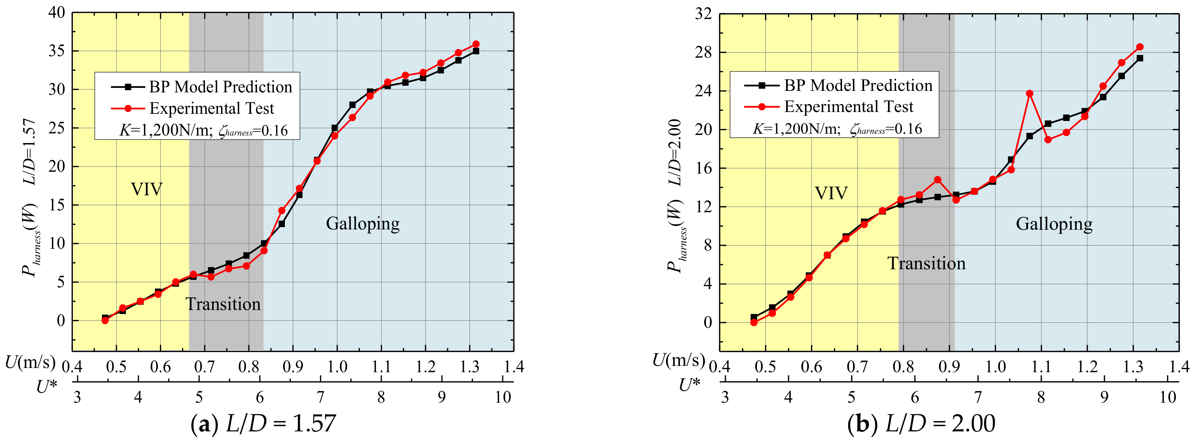
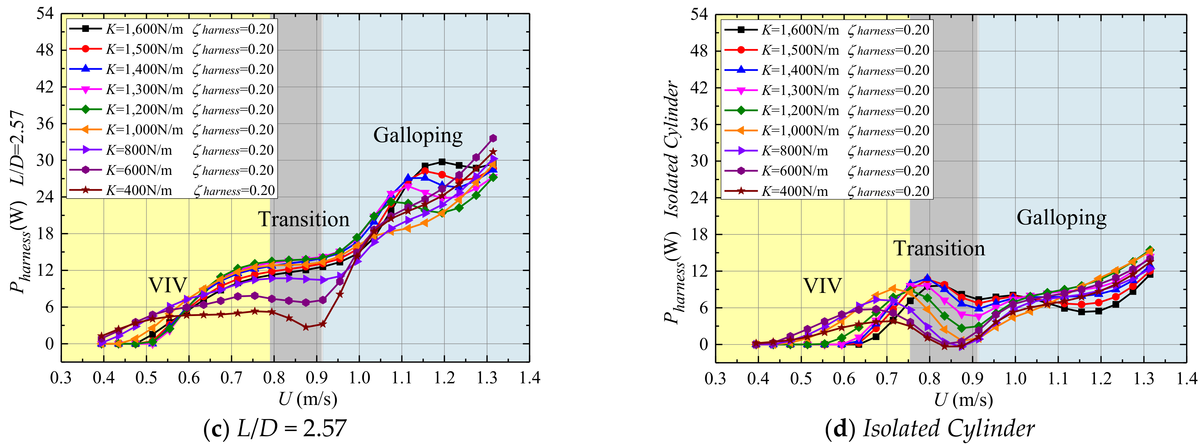
The velocity range of the VIV region for all surrogate models is: 0.39 m/s < U < 0.67 m/s for L/D = 1.57, 0.39 m/s < U < 0.79 m/s for L/D = 2.00 and 2.57, and 0.39 < U < 0.75 m/s for isolated cylinder. As can be seen in Figure 9a, Figure 10a, Figure 11a and Figure 12a, for almost every ζ_harness within the range of 0.04–0.30, increasing the flow velocity in VIV is accompanied by an increase in P_harness. In addition, the coverage range of the VIV-galloping transition region is: 0.79 m/s < U < 0.91 m/s for L/D = 2.57, 0.75 m/s < U < 0.87 m/s for the isolated single cylinder. An interesting phenomenon is that the cases of spacing ratio L/D = 1.57 and 2.00 both have no obvious transition region owing to the positive synergy between two closely spaced oscillators. Nevertheless, the same phenomenon that occurs with a single-cylinder is that for L/D = 2.57, the dropping tendency of P_harness becomes obvious in the transition region. In galloping, for all spacing ratios, P_harness continually increases with the increase of velocity. The above results are highly consistent with the experimental results in [23], indicating that these surrogate models have high accuracy. It should be pointed out that the area covered in gray in Figure 9, Figure 10, Figure 11 and Figure 12 represents the transition region.

(b)

For L/D = 1.57, Figure 9a shows that, with the increase of damping within the range of 0.20–0.30, the variation of P_harness is negligible. Figure 9b illustrates that, in the VIV range, increasing the damping from 0.20 to 0.30 will translate the curve of η_harness to higher velocity and is followed by a significant decrease in η_harness. The above phenomenon is owing to the negative interaction between two tandem cylinders in the sense that the higher damping limits the oscillating amplitude of the downstream cylinder, which is then shielded by the upstream cylinder. As shown in Figure 9b, the optimal η_harness occurs at the upper branch of VIV, and as the damping ratio increases from 0.2 to 0.3, the optimal efficiency increases as well. For instance, the optimal efficiency changes from 40.82% (K = 1200 N/m, ζ_harness = 0.20, U = 0.59 m/s) to 50.51% (K = 1200 N/m, ζ_harness = 0.30, U = 0.71 m/s). Additionally, for U > 0.71 m/s, increasing ζ_harness results in an obvious increase in η_harness on account of the decrease of the amplitude of oscillation. According to Equation (3), the lower amplitude reduces the value of P_Fluid in the denominator of the efficiency.

(c)

For L/D = 2.00: Different from the variation trend of P_harness in Figure 9a, as shown in Figure 10a, increase of ζ_harness in the range of 0.20–0.30 has an obvious influence on the variation of P_harness. Specifically, in the VIV upper branch (0.59 m/s < U < 0.79 m/s), as ζ_harness increases, the corresponding P_harness decreases. However, using the transition region as a turning point, in galloping (U > 0.91 m/s), increasing ζ_harness increases the harnessed power with the maximum predicted value of P_harness is 34.73W (K = 800 N/m, ζ_harness = 0.30, U = 1.31 m/s). Figure 10b shows that, except for the initial VIV branch, in all selected FIO regions, as ζ_harness increases within the range 0.04 < ζ_harness < 0.30, the corresponding η_harness increases. As the harnessing damping ratio increases from 0.20 to 0.30, the increment rate of harnessing efficiency will reach up to 59.52% at U = 0.71 m/s, and the maximum harnessing efficiency is 68.78% at U = 0.63 m/s.

(d)

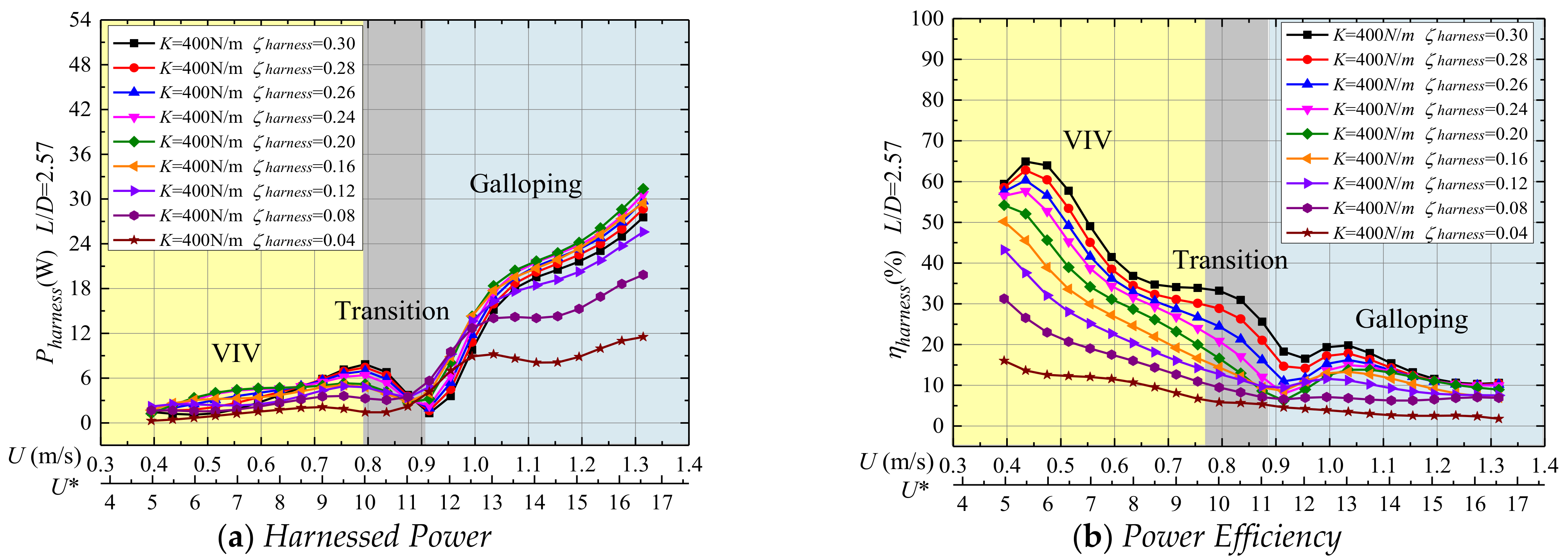
For L/D = 2.57: Being different from the predicted results for L/D = 1.57 and 2.00, for L/D = 2.57, in the VIV initial stage and the entire galloping region, the value of P_harness shows a drop downtrend as ζ_harness increases from 0.20 to 0.30, as shown in Figure 11a. Here, the optimal harnessed power changes from 31.37 W (K = 400 N/m, ζ_harness = 0.20) to 27.54 W (K = 400 N/m, ζ_harness = 0.30) at U = 1.31 m/s. In contrast, it is found that increasing the harnessing damping ratio from 0.20 to 0.30 is followed by an increase of power efficiency in the whole FIO region except at the end region of galloping. For instance, the efficiency changes from 52.09% (K = 400 N/m, ζ_harness = 0.20) to 64.92% (K = 400 N/m, ζ_harness = 0.30) at U = 0.43 m/s. Due to the low spring stiffness (K = 400 N/m), the initial velocity of power harvesting is lower than 0.39m/s. Besides that, the amplitude at low velocity has a relative low value, resulting in high efficiency. As mentioned above, for two tandem cylinders with spacing ratio L/D = 2.57 and K = 400 N/m, it can be observed that increasing the damping ratio from 0.20 to 0.30 will decrease the harnessed power; however, it enhances the power efficiency of the VIVACE Converter.

(e)

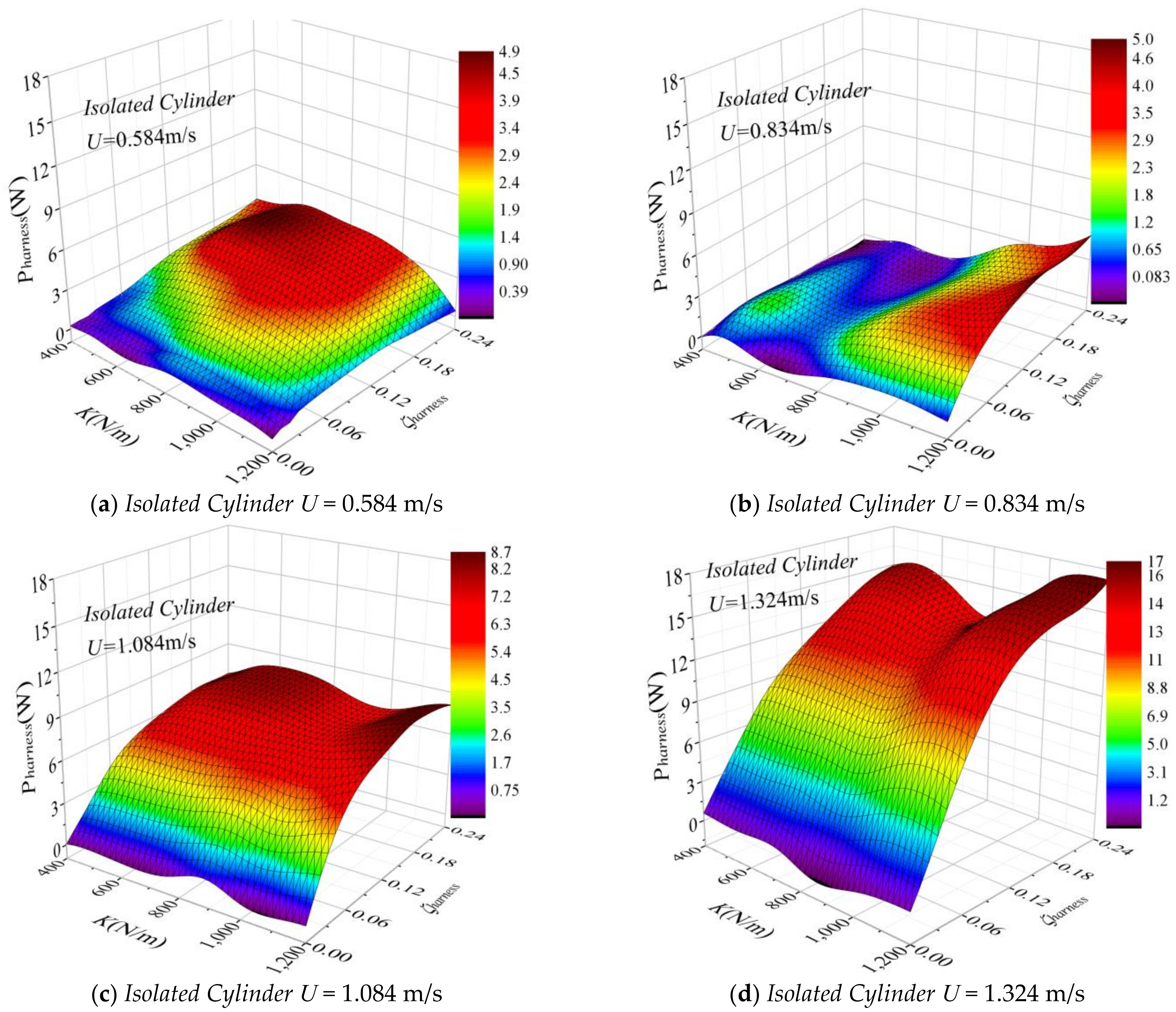
For an isolated cylinder in general, with the increase of spacing ratio, the interaction between the upstream cylinder and downstream cylinder becomes weaker. Therefore, the changes of curves of harnessed power between the spacing ratio of L/D = 2.57 and the isolated single-cylinder cases are similar. However, in this section, the selected fixed stiffness for isolated cylinder and two cylinders with tandem spacing ratio L/D = 2.57 are different. Thus, a large difference in oscillating response exists between these two cases. As we can see in Figure 12a, except for the initial galloping region, the value of P_harness decreases with the increase of harnessing damping ratio (0.2 < ζ_harness < 0.30). Moreover, as ζ_harness increases, the reduction between two adjacent damping ratios increases. Because of the large decrease in P_harness, the corresponding η_harness decreases as well when the damping ratio increases.

(f)

Comparing the power efficiency between the four cases (spacing ratio of L/D = 1.57, 2.00, 2.57 and isolated single cylinder), it is observed that the efficiency of tandem cylinders is much larger than that of the isolated cylinder. For L/D = 2.00, the optimal efficiency for K = 800 N/m and ζ_harness = 0.04–0.30, reaches 1.91 times the hydrokinetic power efficiency of one isolated cylinder. As the spacing ratio increases from 1.57 to 2.00 to 2.57, the optimal efficiency increases from 50.51% to 68.78% to 64.92%, indicating that the smaller spacing of 1.57 induces a negative effect on the power efficiency due to the strong interaction between the two cylinders.

4.2. Effect of Spring Stiffness on Power and Efficiency

Figure 13, shows the two-dimensional diagrams of prediction-results of P_harness with incoming flow velocity (0.39 m/s < U < 1.31 m/s), for the three spacing values of L/D = 1.57, 2.00, 2.57 and the isolated single-cylinder case, respectively. K is the parameter in Figure 13. In order to prevent excessive load on the timing belt of the Vck system, the spring stiffness was allowed to expand from 400–1200 N/m to 400–1600 N/m only. As demonstrated by Sun et al. [23], the harnessing damping ratio of 0.20 is conducive to obtaining the highest values of P_harness for the cases of these three spacing ratios. Therefore, ζ_harness = 0.20 is chosen as a fixed value in order to reduce the variable and control parameter so as to better analyze the impact of K on P_harness. The following results can be observed:

(a)

As shown in Figure 13a–d, in the VIV region, with the increase of flow velocity, the value of P_harness increases. An important finding is that, for the spacing ratio L/D = 1.57 and 2.00, the transition region is not apparent due to the close spacing between the cylinders. Contrary, the spacing ratio L/D = 2.57 and the isolated single-cylinder have a relatively obvious transition. Therefore, the correctness of surrogate models has verified again.

(b)

For L/D = 1.57: As shown in Figure 13a, the power for K = 400–1200 N/m in the VIV region (0.39 m/s ≤ U ≤ 0.67 m/s) and the galloping region have, respectively, approximate and lower values than that of the K = 1200–1600 N/m. More concretely, when U > 0.71 m/s, as K increases from 1200 N/m to 1600 N/m, the power increases; and the optimal power changes from 39 W (K = 1200 N/m, ζ_harness = 0.20, U = 1.31 m/s) to 44.74 W (K = 1600 N/m, ζ_harness = 0.20, U = 1.11 m/s). However, when U > 1.27 m/s, the power of high stiffness case have the approximate values. Considering the above analysis, selecting the stiffness in the range of 1200 N/m < K < 1,600N/m in galloping improves power harvesting. It is also observed that, for L/D = 1.57, increasing K increases power harvesting.

(c)

For L/D = 2.00: As shown in Figure 13b, considering the spring stiffness, all the curves of P_harness show a similar tendency. Moreover, in galloping, two local peaks of P_harness appear at the K = 800 N/m and 1000 N/m, respectively. This phenomenon of K = 800 N/m is in good agreement with the experimental data [23]. Almost in all cases, in the VIV upper branch and the galloping region, the harnessed power shows the downward trend with increase of K in the range 1200 N/m < K < 1600 N/m. Nevertheless, in galloping, the decrement of P_harness between adjacent stiffness values is small. In consequence, for a given harnessing damping ratio of 0.20, increasing K from 1200 N/m to 1600 N/m is adverse to the value of P_harness.

(d)

For L/D = 2.57: As shown in Figure 13c, at low flow velocity (0.39 m/s < U < 0.51 m/s), the VIVACE Converter cannot initiate FIO and, thus, cannot harvest any power at high spring stiffness (1200 N/m < K < 1600 N/m). FIO initiates with VIV a little before the natural frequency of the system in quiescent water; thus, higher stiffness values start FIO at higher flow velocity. This phenomenon is different from that of the low spacing ratio values of L/D = 1.57 and 2.00. From the VIV upper branch to the initial stage of galloping, as K increases within the range 1200 N/m < K < 1600 N/m, the harnessed power decreases. In the end galloping (1.11 m/s ≤ U ≤ 1.31 m/s), when U = 1.19 m/s, the value of P_harness rapidly increases from 21.40W (K = 1200 N/m, ζ_harness = 0.20) to 29.73 W (K = 1600 N/m, ζ_harness = 0.20) as stiffness increases. However, combined with the variable trend of harnessed power when K = 400–1200 N/m in Figure 13c, it can be concluded that expanding the K from 400–1200 N/m to 400–1600 N/m is not conducive to increase the power harvesting at low flow velocities. Increase can be observed in the end region of galloping (1.07 m/s < U < 1.23 m/s).

(e)

For an isolated cylinder, as shown in Figure 13d, an isolated single-cylinder with high spring stiffness cannot induce VIV at low flow velocity due to the high natural frequency of the oscillator in quiescent water, f_n,water. This is due to the strong restoring force provided by the hard spring. For the same reason, as K increases from 600 N/m to 1600 N/m, the initial flow velocity of power harvesting increases as well. This increase is expected to follow the square root of K as in f_n,water. Of course, the curve of P_harness of the isolated single cylinder will shift to higher velocity. Therefore, in the VIV region, expanding the selected range of K from 400–1200 N/m to 400–1600 N/m has no effect on the increase of P_harness. On the contrary, in the transition region and initial galloping, expanding the selected range of K is beneficial for enhancing the power harvesting. The range of synchronization in VIV shifts to the right proportionally to the square root of K while galloping initiation is independent of K. When U = 0.83–1.11 m/s, as K increases from 1200 N/m to 1600 N/m, P_harness increases. In the transition region, the optimal harnessed power can reach up to 10.82W (K = 1400 N/m, ζ_harness = 0.20, U = 0.79 m/s), which is 10.3 times the harnessed power for K = 400 N/m (P_harness = 1.05W, ζ_harness = 0.20, U = 0.79 m/s). Besides that, taking U = 1.03 m/s as the turning point, when U > 1.03 m/s, P_harness shows a drop tendency as K increases from 1200 to 1600 N/m.

4.3. Optimal Power and Efficiency Envelope for Two Cylinders in Tandem

To further analyze the performance of this Current Energy Converter (CEC) consisting of two cylinders in tandem, the above established four surrogate models are used to find the optimal harnessed power and optimal power efficiency. This is done for each available flow velocity: i.e., U = 0.39–1.31 m/s, in increments of 0.04 m/s. It should be pointed out that the optimal values of P_harness and η_harness can be found by introducing the traditional method of grid searching based on the modeling of power and efficiency in a series of spring stiffness and harnessing damping ratio values. The spring stiffness and harnessing damping ratio are, respectively, selected in the ranges of K = 400–1200 N/m in 10N/m intervals and ζ_harness = 0.00–0.30 in 0.005 increments. Selecting too large an interval would reduce the accuracy of the optimal value. On the other hand, selecting too small an interval would result in unnecessary calculations as the power and efficiency of the original experimental data were not measured in such small increments. The optimal power and efficiency for each velocity are shown in Figure 14a,b, respectively. The corresponding optimal parameters are presented in Appendix A,

Table A1. Parameters for optimal harnessed power for two tandem cylinders with spacing: L/D = 1.57, 2.00 and 2.57.

	Optimal Harvested Power (W)			Stiffness K [N/m]			Harnessing Damping Ratio ζharness
U [m/s]	L/D = 1.57	L/D = 2.00	L/D = 2.57	L/D = 1.57	L/D = 2.00	L/D = 2.57	L/D = 1.57	L/D = 2.00	L/D = 2.57
0.39	1.23	4.18	2.38	700	400	500	0.01	0.3	0.105
0.43	2.21	5.26	3.02	680	400	540	0.13	0.3	0.12
0.47	3.34	5.88	3.67	680	420	580	0.13	0.3	0.16
0.51	4.15	6.41	5.01	680	440	720	0.135	0.3	0.2
0.55	5.13	7.19	6.53	720	660	740	0.24	0.225	0.21
0.59	6.42	8.37	7.88	720	600	760	0.24	0.3	0.225
0.63	7.32	10.81	9.42	700	580	960	0.23	0.3	0.23
0.67	8.05	12.94	11.29	680	580	980	0.22	0.3	0.24
0.71	8.82	14.54	12.88	660	600	1080	0.21	0.3	0.235
0.75	9.65	15.78	13.76	660	620	1120	0.205	0.3	0.24
0.79	10.64	16.89	14.27	680	640	1200	0.205	0.3	0.255
0.83	12.11	17.89	14.37	820	660	1200	0.165	0.3	0.255
0.87	15.00	18.74	14.18	840	680	1200	0.165	0.3	0.25
0.91	18.61	19.65	14.08	860	680	1200	0.165	0.3	0.21
0.95	22.19	21.03	15.41	880	700	1080	0.17	0.3	0.175
0.99	25.82	23.23	18.07	1200	700	1100	0.25	0.3	0.17
1.03	29.34	24.75	21.13	1200	700	1180	0.25	0.3	0.18
1.07	31.83	25.00	23.36	1200	700	1200	0.255	0.3	0.19
1.11	33.88	24.90	23.08	1200	720	1200	0.265	0.3	0.19
1.15	35.96	25.45	23.84	1200	760	640	0.28	0.3	0.2
1.19	38.01	26.94	25.50	1200	760	620	0.29	0.3	0.185
1.23	39.50	29.65	27.77	1200	780	600	0.295	0.3	0.185
1.27	40.28	32.73	30.58	1200	780	600	0.285	0.3	0.19
1.31	40.62	34.99	33.61	1200	780	600	0.275	0.3	0.2

and

Table A2. Parameters for optimal converted efficiency for two tandem cylinders with spacing: L/D = 1.57, 2.00 and 2.57.

	Optimal Converted Efficiency (%)			Stiffness K [N/m]			Harnessing Damping Ratio ζharness
U [m/s]	L/D = 1.57	L/D = 2.00	L/D = 2.57	L/D = 1.57	L/D = 2.00	L/D = 2.57	L/D = 1.57	L/D = 2.00	L/D = 2.57
0.39	29.95	46.86	54.03	460	400	400	0.16	0.195	0.235
0.43	33.70	51.65	57.71	460	440	400	0.215	0.22	0.3
0.47	38.87	53.72	58.37	480	460	400	0.25	0.235	0.3
0.51	42.94	58.74	60.04	820	640	720	0.23	0.3	0.23
0.55	48.06	70.50	62.00	740	660	800	0.295	0.3	0.245
0.59	50.33	73.14	64.24	800	680	1000	0.3	0.3	0.3
0.63	49.54	68.92	67.61	980	680	1060	0.3	0.3	0.3
0.67	49.41	62.04	68.84	1120	680	1140	0.3	0.3	0.3
0.71	50.51	59.31	69.44	1200	1200	1200	0.3	0.3	0.3
0.75	49.05	56.81	68.26	1200	1200	1200	0.3	0.3	0.3
0.79	45.74	52.07	64.15	1200	1200	1200	0.3	0.3	0.3
0.83	41.95	47.33	55.98	1200	1200	1200	0.3	0.3	0.3
0.87	38.50	43.07	45.14	1200	1200	1200	0.3	0.3	0.3
0.91	35.75	38.97	34.66	1200	1200	1200	0.3	0.3	0.3
0.95	33.71	34.78	29.64	1200	1200	1180	0.3	0.3	0.21
0.99	32.24	30.61	27.56	1200	1200	1180	0.3	0.3	0.215
1.03	31.12	26.76	25.70	1200	1200	1200	0.3	0.3	0.22
1.07	30.62	24.14	23.84	1200	680	1200	0.255	0.23	0.225
1.11	30.19	22.51	22.29	1200	700	980	0.25	0.23	0.3
1.15	29.61	21.38	21.20	1200	760	1000	0.25	0.3	0.3
1.19	28.79	21.59	19.91	1200	780	1020	0.25	0.3	0.3
1.23	27.67	22.30	18.61	1200	800	1000	0.255	0.3	0.3
1.27	26.22	22.92	18.51	1200	800	660	0.265	0.3	0.3
1.31	24.61	23.29	19.37	1200	820	640	0.285	0.3	0.3

.

The following observations can be made:

(a)

In the VIV region (0.39 m/s < U < 0.79 m/s), a continuous growth of harnessed power can be observed for spacing L/D = 1.57, 2.00 and 2.57. Besides that, the power for L/D = 2.00 is higher than that of the other two spacing ratios, as shown in Figure 14a. In this region, the maximum power is: P_harness = 10.64 W (L/D = 1.57, K = 680 N/m, ζ_harness = 0.205), P_harness = 16.89 W (L/D = 2.00, K = 640 N/m, ζ_harness = 0.30), P_harness = 14.27 W (L/D = 2.57, K = 1200 N/m, ζ_harness = 0.255).

(b)

In the initial VIV branch (U < 0.47 m/s), as shown in Table A1, the combination of lower stiffness with lower harnessing damping ratio stimulates the onset of VIV for lower velocity U < 0.39 m/s, which is consistent with the conclusion in Ref. [23]. Additionally, for spacing L/D = 2.00 and 2.57, increasing the flow velocity is accompanied by an increase in power efficiency. The efficiency exhibits a local maximum after which it decreases as shown in Figure 14b. The maximum efficiency for L/D = 2.00 and 2.57 are, respectively, η_harness = 73.14% (L/D = 2.00, K = 680 N/m, ζ_harness = 0.30, U = 0.59 m/s) and η_harness = 69.44% (L/D = 2.57, K = 1200 N/m, ζ_harness = 0.30, U = 0.71 m/s), as shown in Table A2. That optimum is located near the end of the VIV upper branch. An interesting phenomenon can be observed that there are two local maxima for spacing L/D = 1.57. The higher one is η_harness = 50.51% (L/D = 1.57, K = 1200 N/m, ζ_harness = 0.30, U = 0.71 m/s). The local optima can be explained by studying carefully Equations (4)–(6). The swept area dominating the denominator in Equation (3) changes at a different rate than the cylinder velocity square dominating the numerator in Equation (4).

(c)

In the transition region from VIV to galloping (0.79 m/s < U < 0.91 m/s), power harvesting for spacing L/D = 1.57 and 2.00 almost have a direct proportional relation with flow velocity. For spacing L/D = 2.57, however, a downward trend is observed. With increasing flow velocity, the efficiency decreases. Before the onset of galloping, the power efficiency for L/D = 1.57 is lower than that of the other two spacing ratios.

(d)

In galloping (U > 0.91 m/s), increasing the flow velocity is beneficial for power harvesting; however, it is detrimental to the power efficiency due to the dramatic increase in amplitude and thus, swept area. When U > 0.95 m/s, the lowest spacing results in highest power or efficiency with higher spring stiffness. In this region, the maximum power is: P_harness = 40.62 W (L/D = 1.57, K = 1200 N/m, ζ_harness = 0.275, U = 1.31 m/s), P_harness = 34.99 W (L/D = 2.00, K = 780 N/m, ζ_harness = 0.30, U = 1.31 m/s), P_harness = 33.61 W (L/D = 2.57, K = 600 N/m, ζ_harness = 0.20, U = 1.31 m/s).

(e)

To better analyze the synergy effect of the two tandem cylinders, the optimal harnessed power and efficiency of the isolated single cylinder are also modeled, and are added in Figure 14a,b, respectively. The corresponding optimal parameters for an isolated cylinder are presented in Appendix A,

Table A3. Parameters of optimal harnessed power and efficiency for single cylinder.

	Parameters for Optimal Pharness			Parameters for Optimal ηharness
U [m/s]	Pharness [W]	K [N/m]	ζharness	ηharness [%]	K [N/m]	ζharness
0.43	1.13	400	0.155	25.83	780	0.3
0.47	1.51	400	0.15	26.36	820	0.3
0.51	2.55	600	0.185	33.40	620	0.22
0.55	3.89	600	0.18	41.34	680	0.22
0.59	5.15	640	0.185	45.09	720	0.24
0.63	6.41	880	0.225	46.10	880	0.24
0.67	8.50	940	0.245	47.06	920	0.28
0.71	10.00	980	0.26	45.56	960	0.3
0.75	9.66	1020	0.275	39.22	1020	0.3
0.79	7.63	1200	0.22	31.07	1200	0.24
0.83	5.91	1200	0.3	21.10	1200	0.28
0.87	4.20	1200	0.3	12.47	1200	0.3
0.91	5.22	1200	0.105	9.72	1200	0.3
0.95	6.70	1200	0.115	11.97	1200	0.3
0.99	7.43	1200	0.125	15.20	1200	0.3
1.03	7.94	1200	0.165	16.55	1200	0.3
1.07	8.56	1200	0.175	16.08	1200	0.3
1.11	9.15	1200	0.17	14.85	1200	0.3
1.15	10.14	1080	0.175	13.57	1200	0.3
1.19	11.61	1080	0.18	12.50	1200	0.3
1.23	13.35	1140	0.3	11.70	1200	0.3
1.27	16.61	1180	0.3	11.35	1040	0.3
1.31	19.93	1200	0.3	11.19	1060	0.3

. Specifically, the green line in Figure 14 represents the maximum optimal value at each velocity for three cases of the tandem cylinder. As shown in Figure 14a, it can be observed that at almost every selected flow velocity, the optimal harnessed power of two tandem cylinders has a higher value than that of the isolated cylinder. More concretely, the two cylinders in tandem can harness 2.01–4.67 times the power of the isolated cylinder at the selected range of flow velocity except for the upper branch of VIV. Further, the two tandem cylinders can achieve 1.46–4.01 times the efficiency of the isolated one.

Based on the analysis in Section 4.1, in order to further verify that the wider range of damping ratio (0.00 < ζ_harness < 0.30) has better performance than that of the original range (0.00 < ζ_harness < 0.24) [23], a similar surrogate model as the one developed in Section 4.3 is established by replacing the wider range of ζ_harness by the narrower one. Figure 15a shows that extending the range from 0.00–0.24 to 0.00–0.30 has little impact on the optimal harnessed power for each flow velocity, except for the spacing L/D = 2.00. For L/D = 2.00, the maximum increment will reach up to 5.30 W at U = 0.95 m/s. However, this operation for ζ_harness obviously increases the optimal power efficiency, especially in the upper branch of the VIV region and a transition region between VIV and galloping, as shown in Figure 15b. Therefore, extending the harnessing damping ratio from 0.00–0.24 to 0.00–0.30 has a positive influence on optimal power harvesting and optimal power efficiency.

5. Conclusions

The harnessed power and converting efficiency of the VIVACE hydrokinetic energy Converter with two tandem cylinders were modeled by a surrogate-based model established by the BP neural network method. The design parameters are flow velocity, harnessing damping ratio, spring stiffness, and spacing ratio. Modeling is based on the experimental data from tests conducted in the LTFSW channel of the MRELab of the University of Michigan. The major conclusions can be summarized as follows:

(1)

The structure of BPNN is simpler than that of RBFNN when solving the problems with the same precision requirements, and the number of hidden layer neurons of RBF neural network is much higher than that of BPNN when there are more training samples, which makes the complexity and computation of RBFNN increase greatly. Therefore, this paper selected the BPNN to establish the surrogate model of the VIVACE Converter.

(2)

By training and testing experimental sample data, an efficient and accurate surrogate model of the VIVACE Converter was established. The harnessed power and corresponding efficiency of the Converter can be predicted accurately under different combinations of incoming flow velocity, spacing ratio, spring stiffness, and harnessing damping ratio.

(3)

Under a specified spring stiffness, expanding the selected range of harnessing damping ratio from 0–0.24 to 0–0.30 results in no appreciable power increase for the isolated single cylinder and two tandem cylinders for spacing (L/D = 1.57 and 2.57). On the contrary, the corresponding efficiency increases significantly due to the decreased oscillating amplitude, which directly results in decrease of P_Fluid. Specifically, for L/D = 2.57, the efficiency changes from 52.09% (K = 400 N/m, ζ_harness = 0.24) to 64.92% (K = 400 N/m, ζ_harness = 0.30) at U = 0.43 m/s.

(4)

Increasing the spring stiffness range from 400–1200 N/m to 400–1600 N/m improves the ability of power harvesting in galloping for the VIVACE Converter with two tandem cylinders (L/D = 1.57).

(5)

Due to synergy between two tandem cylinders, the VIVACE Converter with two tandem cylinders has a better performance of power harvesting compared to that of the isolated single cylinder. Analysis of the optimal harnessed power and efficiency shows that the two tandem cylinders can harness 2.01–4.67 times the power of the isolated cylinder. In addition, two tandem cylinders can achieve 1.46–4.01 times the efficiency of the isolated one.

The results provide valuable insight into the parametric dependence of power and efficiency of a two-oscillator converter on spacing, spring-stiffness, damping ratio, and flow velocity. What may be even more valuable though, is the potential implementation of the developed model in engineering applications. That is to say, at each flow velocity, selecting appropriate optimal spacing ratio, spring stiffness and harnessing damping ratio can induce the optimal harvested power or efficiency in the actual current. Specifically:

(a)

During field-tests or in commercial use of a two-cylinder VIVACE Converter, flow speed changes. To maintain near-optimal performance, parameters should be adjusted. The derived model can provide real-time guidance to that effect.

(b)

The model can be tested against field-data and be modified or expanded accordingly.

(c)

This Converter has been studied experimentally and with field-tests for over a decade using many different parameters and various size oscillators. One of the most powerful ways of increasing its harnessed power or its harnessing efficiency is an adaptive change of parameters. For example, in [18] the spring stiffness was adjusted based on response amplitude. In [25], the damping was adjusted based on the speed of the oscillating cylinder.

(d)

One of the greatest advantages of the VIVACE Converter is that it is fish-friendly because it operates on alternating lift like fish rather than steady lift like wings. Nevertheless, until recently [6], there was no physics-based mathematical model of the alternating lift force in VIV or galloping, which is required for proper control. The model developed in this paper serves as a guide for a numerical control model.

(e)

Recently [13], a physics-based force model was developed following the revealing of an eigen-relation at the interface between fluid and structure in VIV and galloping. The eigen-relation matched experimental results with extreme accuracy changing completely the modeling of VIV and galloping. On the other hand, an eigen-relation is amplitude and energy independent while control requires a specific amplitude input for modeling. That can be provided by the model developed in this paper.

(f)

It should be pointed out that in future research, RBFNN method can be considered to establish the surrogate model of VIVACE Converter with double series cylinder and compared with BPNN, it must have a certain research value.

References

1. Bull, S.R. Renewable Energy Today and Tomorrow. IEEE Proc. 2001, 89, 1216–1226. [Google Scholar] [CrossRef]
2. Lund, H. Renewable energy strategies for sustainable development. Energy 2007, 32, 912–919. [Google Scholar] [CrossRef] [Green Version]
3. Gielen, D.; Boshell, F.; Saygin, D.; Bazilian, M.D.; Wagner, N.; Gorini, R. The role of renewable energy in the global energy transformation. Energy Strategy Rev. 2019, 24, 38–50. [Google Scholar] [CrossRef]
4. Hongda, M. Research on Power Control Method of Oscillating Float Type Ocean Wave Energy Power Generation. IOP Conf. Ser. Earth Environ. Sci. 2020, 546, 022027. [Google Scholar] [CrossRef]
5. Wang, J.L.; Su, Z.; Li, H.; Ding, L.; Zhu, H.J.; Gaidai, O. Imposing a wake effect to improve clean marine energy harvesting by flow-induced vibrations. Ocean Eng. 2020, 208, 107455. [Google Scholar] [CrossRef]
6. You, Y.G.; Li, W.; Liu, W.M.; Li, X.Y.; Wu, F. Development Status and Perspective of Marine Energy Conversion Systems. Autom. Electr. Power Syst. 2010, 34, 1–12. [Google Scholar]
7. Bernitsas, M.M. Harvesting Energy by Flow Included Motions. In Springer Handbook of Ocean Engineering; Dhanak, M.R., Xiros, N.I., Eds.; Springer: Berlin/Heidelberg, Germany, 2016; Chapter 47; pp. 1163–1244. ISBN 978-3-319-16648-3. [Google Scholar]
8. VanZwieten, J.H.; Smentek-Duerr, A.E.; Alsenas, G.M.; Hanson, H.P. Global Ocean Current Energy Assennment: An Initial Look. In Proceedings of the 1st Marine Energy Technology Symposium, Washington, DC, USA, 10–11 April 2013. [Google Scholar]
9. Yang, L.F.; Haas, K.A.; Fritz, H.M. Theoretical Assessment of Ocean Current Energy Potential for the Gulf Stream System. Mar. Technol. Soc. J. 2013, 47, 101–112. [Google Scholar] [CrossRef]
10. Martinez, R.; Ordonez-Sanchez, S.; Matthem, A.; Catherine, L.; Tim, O.D.; Gregory, G.; Benoit, G.; Cameron, J. Analysis of the effects of control strategies and wave climates on the loading and performance of a laboratory scale horizontal axis tidal turbine. Ocean Eng. 2020, 212, 107713. [Google Scholar] [CrossRef]
11. Sleiti, A.K. Overview of Tidal Power Technology. Energy Sources Part B Econ. Plan. Policy 2015, 10, 8–13. [Google Scholar] [CrossRef]
12. Williamson, C.H.K.; Govardhan, R. Vortex-Induced Vibrations. Annu. Rev. Fluid Mech. 2004, 36, 413–455. [Google Scholar] [CrossRef] [Green Version]
13. Bernitsas, M.M.; Ofuegbe, J.; Chen, J.-U.; Sun, H. Eigen-Relation for Flow Induced Oscillations (VIV & Galloping) Revealed at the Fluid-Structure Interface. In Proceedings of the 38th OMAE 2019 Conference, Glasgow, Scotland, 9–14 June 2019. Paper #96823. [Google Scholar]
14. Jauvtis, N.; Williamson, C.H.K. Vortex-induced vibration of a cylinder with two degrees of freedom. J. Fluids Struct. 2003, 17, 1035–1042. [Google Scholar] [CrossRef]
15. Ji, C.N.; Li, F.F.; Chen, W.L.; Song, X.Y. Progress and Prospect of the Study on Vortex-Induced Vibration of Circular Cylinders. J. Ocean Technol. 2015, 34, 106–118. [Google Scholar]
16. Bernitsas, M.M.; Raghavan, K.; Ben-Simon, Y.; Garcia, E.M.H. VIVACE (vortex induced vibration aquatic clean energy): A new concept in generation of clean and renewable energy from fluid flow. In Proceedings of the 25th International Conference on Offshore Mechanicals and Arctic Engineering-OMAE, Hamburg, Gemany, 4–9 June 2006. [Google Scholar]
17. Prasanth, T.K.; Mittal, S. Flow-induced oscillation of two circular cylinders in tandem arrangement at low Re. J. Fluids Struct. 2009, 25, 1029–1048. [Google Scholar] [CrossRef]
18. Ma, C.H.; Sun, H.; Nowakowski, G.; Mauer, E.; Bernitsas, M.M. Nonlinear piecewise restoring force in hydrokinetic power conversion using flow induced motions of single cylinder. Ocean Eng. 2016, 128, 1–12. [Google Scholar] [CrossRef] [Green Version]
19. Park, H.; Bernitsas, M.M.; Kumar, A.R. Using the map of passive turbulence control to flow induced motions to suppress circular cylinder motion at 31,000 ≤ Re ≤ 120,000. J. Offshore Mech. Arctic Eng. Trans. ASME 2012, 134, V007T08A003. [Google Scholar]
20. Park, H.R.; Kumar, R.A.; Bernitsas, M.M. Enhancement of flow induced motions of rigid circular cylinder on springs by localized surface roughness at 3 × 10⁴ ≤ Re ≤ 1.2 × 10⁵. Ocean Eng. 2013, 72, 403–415. [Google Scholar] [CrossRef]
21. Raghavan, K.; Bernitsas, M.M. Enhancement of high damping VIV though roughness distribution for energy harnessing at 8 × 10³ < Re < 1.5 × 10⁵. In Proceedings of the 27th International Conference on Offshore Mechanicals and Arctic Engineering-OMAE, Estoril, Portugal, 15–20 June 2008. [Google Scholar]
22. Sun, H.; Kim, E.S.; Nowakowski, G.; Mauer, E.; Bernitsas, M.M. Effect of mass-ratio, damping, and stiffness on optimal kydrokinetic energy conversion of a single, rough cylinder in flow induced motions. Renew. Energy 2016, 99, 936–959. [Google Scholar] [CrossRef] [Green Version]
23. Sun, H.; Ma, C.H.; Kim, E.S.; Nowakowski, G.; Mauer, E.; Bernitsas, M.M. Hydrokinetic energy conversion by two rough tandem-cylinders in flow induced motions: Effect of spacing and stiffness. Renew. Energy 2017, 107, 61–80. [Google Scholar] [CrossRef] [Green Version]
24. Ding, L.; Zhang, L.; Bernitsas, M.M. Numerical simulation and experimental validation for energy harvesting of single-cylinder VIVACE converter with passive turbulence control. Renew. Energy 2016, 85, 1246–1259. [Google Scholar] [CrossRef] [Green Version]
25. Sun, H.; Bernitsas, M.M.; Turkol, M. Adaptive harnessing damping in hydrokinetic energy conversion by two rough tandem-cylinders using flow-induced vibrations. Renew. Energy 2020, 149, 828–860. [Google Scholar] [CrossRef]
26. Lee, J.H.; Bernitsas, M.M. High-damping, high-Reynolds VIV tests for energy harnessing using the VIVACE converter. Ocean Eng. 2011, 38, 1679–1712. [Google Scholar] [CrossRef]
27. Ding, L.; Zhang, L.; Kim, E.S.; Bernitsas, M.M. 2D-URANS vs. Experiments of Flow Induced Motions of Multiple Circular Cylinders with Passive Turbulence Control. J. Fluids Struct. 2015, 54, 612–628. [Google Scholar] [CrossRef] [Green Version]
28. Ding, L.; Zhang, L.; Wu, C.M.; Kim, E.S.; Bernitsas, M.M. Numerical study on the effect of tandem spacing on flow-induced motions of two cylinders with passive turbulence control. J. Offshore Mech. Arctic Eng. 2017, 139, 021801. [Google Scholar] [CrossRef]
29. Wang, G.G.; Shan, S. Review of Metamodeling Techniques in Support of Engineering Design Optimization. J. Mech. Des. 2016, 129, 370–380. [Google Scholar] [CrossRef]
30. Sultan, I.A.; Ahmed, M.R.; Gareth, L.F. Evaluation of slug flow-induced flexural loading in pipelines using a surrogate model. J. Offshore Mech. Arctic Eng. 2013, 135, 031703. [Google Scholar] [CrossRef]
31. Zhang, J.; Chowdhury, S.; Messac, A. An adaptive hybrid surrogate model. Struct. Multidiscip. 2012, 46, 223–238. [Google Scholar] [CrossRef]
32. Matias, S.; Nestor, R.G.; Yang, H.; Shen, W.Z. Aerodynamic wind-turbine rotor design using surrogate modeling and three-dimensional viscous-inviscid interaction technique. Renew. Energy 2016, 93, 620–635. [Google Scholar]
33. Wu, W.H.; Sun, H.; Lv, B.C.; Bernitsas, M.M. Modelling of a hydrokinetic energy converter for flow-induced vibration based on experimental data. Ocean Eng. 2018, 155, 392–410. [Google Scholar] [CrossRef]
34. Broomhead, D.S.; Lowe, D. Radial basis functions, multi-variable functional interpolation and adaptive networks. Royal Radar Est. 1988. [Google Scholar]
35. Yasav, A.K.; Sharma, V.; Malik, H.; Chandel, S.S. Daily array yield prediction of grid-interaction photovoltaic plant using relief attribute evaluator based Radial Basis Function Neural Network. Renew. Sustain. Energy Rev. 2018, 81, 2115–2127. [Google Scholar]
36. Jin, W.; Li, Z.J.; Wei, L.S.; Zhen, H. The improvements of BP neural network learning algorithm. In Proceedings of the 5th International Conference on Signal Processing Proceedings 16th World Computer Congress, Beijing, China, 21–25 August 2000. [Google Scholar]
37. Sadeghi, B.H.M. A BP-neural network predictor model for plastic injection molding process. J. Mater. Process. Technol. 2000, 103, 411–416. [Google Scholar] [CrossRef]
38. Kim, E.S.; Bernitsas, M.M.; Kumar, R.A. Multicylinder Flow-Induced Motions: Enhancement by Passive Turbulence Control at 28,000 < Re < 120,000. J. Offshore Mech. Arctic Eng. 2013, 135, 021802. [Google Scholar]
39. Sun, H.; Kim, E.S.; Bernitsas, P.M.; Bernitsas, M.M. Virtual spring–damping system for flow-induced vibration experiments. J. Offshore Mech. Arctic Eng. 2015, 137, 061801. [Google Scholar] [CrossRef]
40. Shi, Y.W.; Wang, C.K.; Shen, J.F. Utilization and prospect of ocean energy resource in china. Acta Energ. Sol. Sin. 2011, 6, 913–923. [Google Scholar]
41. Kohavi, R. A study of cross-validation and bootstrap for accuracy estimation and model selection. In Proceedings of the International Joint Conference on Artificial Intelligence-IJCAI, Montreal, QC, Canada, 20–25 August 1995; pp. 1137–1145. [Google Scholar]
Figure 1. Two-cylinder VIVACE Converter with Vck: (a) In the LTFSW Channel; (b) Schematic drawing.
Energies 14 00827 g001
Figure 2. Configuration of the turbulence stimulation (PTC) on the cylinder [23].
Energies 14 00827 g002
Figure 3. Schematic diagram of Back Propagation (BP) neural network.
Energies 14 00827 g003
Figure 4. Relation between the RMSE of BP neural network and the number of the hidden layer nodes.
Energies 14 00827 g004
Figure 5. Three evaluation measures of modeling accuracy.
Energies 14 00827 g005
Figure 6. Comparison of Pharness predicted numerically and measured experimentally: (a) L/D = 1.57; (b) L/D = 2.00; (c) L/D = 2.57; (d) Isolated Cylinder.
Energies 14 00827 g006aEnergies 14 00827 g006b
Figure 7. Power harvesting at various K and ζharness based on BP modeling for tandem cylinders with L/D = 2.00: (a) U = 0.584 m/s; (b) U = 0.834 m/s; (c) U = 1.084 m/s; (d) U = 1.324 m/s.
Energies 14 00827 g007aEnergies 14 00827 g007b
Figure 8. Power harvesting at various K and ζharness based on BP modeling for isolated cylinder: (a) U = 0.584 m/s; (b) U = 0.834 m/s; (c) U = 1.084 m/s; (d) U = 1.324 m/s.
Energies 14 00827 g008
Figure 9. (a) Harnessed power and (b) power efficiency of two tandem cylinders with spacing ratio L/D = 1.57; K = 1200 N/m; ζharness = 0.04–0.30.
Energies 14 00827 g009
Figure 10. (a) Harnessed power and (b) power efficiency of two tandem cylinders with spacing ratio L/D = 2.00; K = 800 N/m; ζharness = 0.04–0.30.
Energies 14 00827 g010
Figure 11. (a) Harnessed power and (b) power efficiency of two tandem cylinders with spacing ratio L/D = 2.57; K = 400 N/m, ζharness = 0.04–0.30.
Energies 14 00827 g011
Figure 12. (a) Harnessed power and (b) power efficiency of isolated single cylinder; K = 1200 N/m; ζharness = 0.04–0.30.
Energies 14 00827 g012
Figure 13. Harnessed power of two tandem cylinders with K = 400–1600 N/m and ζharness = 0.20: (a) L/D = 1.57; (b) L/D = 2.00; (c) L/D = 2.57; (d) isolated cylinder.
Energies 14 00827 g013aEnergies 14 00827 g013b
Figure 14. The optimal power and efficiency curves for spacing L/D = 1.57, 2.00 and 2.57: (a) Harnessed power; (b) Power efficiency. Model is based on K = 400–1200 N/m and 0.00 < ζharness < 0.30.
Energies 14 00827 g014
Figure 15. The optimal power and efficiency curves for spacing ratio L/D = 1.57, 2.00 and 2.57: (a) Harnessed power; (b) Power efficiency. Model is based on K = 400–1200 N/m and 0.00 < ζharness < 0.30.
Energies 14 00827 g015