Look Ahead Based Control Strategy for Hydro-Static Drive Wind Turbine Using Dynamic Programming

Abstract

This research paper presents a look-ahead optimal control strategy for a Hydro-static Drive Wind Turbine when look ahead wind speed information is available. The proposed predictive controller is a direct numerical optimizer based on the well established principles of Hamilton-Jacobi-Bellman (Dynamic Programming). Hydro-static transmission based, non-linear model of wind turbine is used in this optimization work. The optimal behavior of the turbine used the non-linearity of aerodynamic maps and hydro-static drive train by a convex combination of state space controller with measurable generator speed and hydraulic motor displacement as scheduling parameters. A comparative analysis between a optimal controller based on Maximum Power Point Tracking (MPPT) algorithm as published in literature and the proposed look ahead based predictive controller is presented. The simulation results show that proposed look ahead strategy offered optimal operation of the wind turbine by closely tracking the optimal tip-speed ratio to maximize capacity factor while also maintaining the hydraulic motor speed close to the desired value to ensure that the frequency of electrical output is constant. It is observed from the simulation results that the proposed predictive controller provided around 3.5% better performance in terms of improving total system losses and harvesting energy as compared to the MPPT algorithm.

1. Introduction

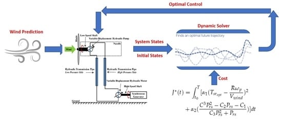
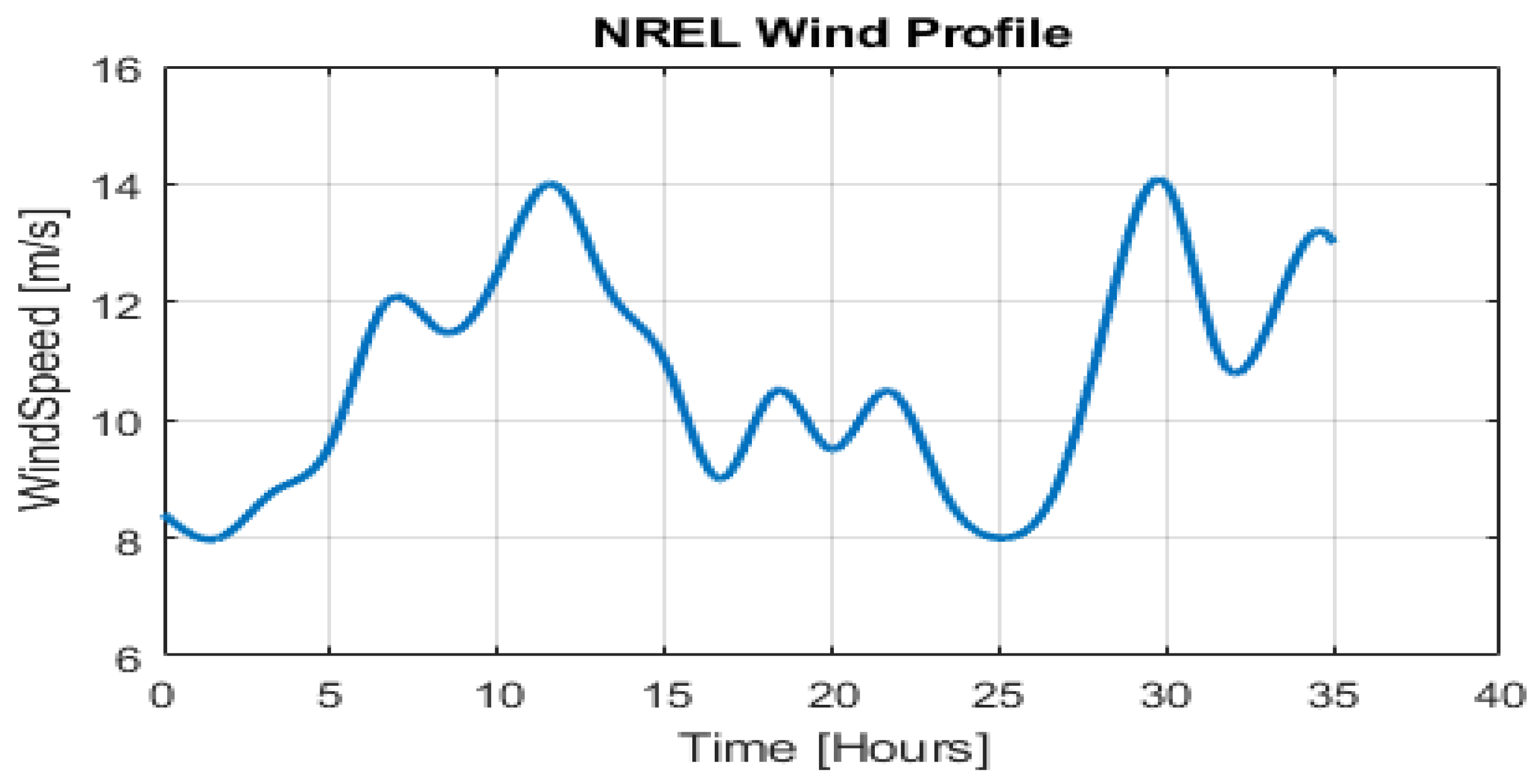
Wind energy harvesting is a key contributor to sustainable energy production in recent years. There is a number of different turbine configurations available with a variety of control methods for each. In this paper an innovative study is carried out to assess the global optimality of a hydro-static drive wind turbine performance using predictive techniques. It is assumed in this work that a reliable prediction of wind speed can be made over a time horizon looking well ahead in time. In this study a window of 35 H is used for simulation complexity. The wind profile is taken from National Renewable Energy Lab (NREL). With the knowledge of look ahead wind speed, a direct numerical method based optimizer is used to solve the problem as a trajectory optimization problem. Dynamic programming is used as the chosen numerical optimizer in this work since it guarantees global optimality based on the direct numerical approach. It is to be noted here that dynamic programming like many other numerical optimizer will not give the reasons for the improvement but rather will indicate that there is possibility of rule based or other controls methods that can be implemented to extract the benefits in embeddable solution. There are three major sections in this paper:

• Implementation and validation of the control oriented model of the hydro-static drive wind turbine based on published literature [1,2,3,4]. This control oriented model will be the baseline for comparison of benefits with the proposed controller. The baseline control oriented model also runs the traditional Pontryagins’s Minimum Principle based Maximum Power Point Tracking algorithm as the control strategy;
• The second section discusses the background of dynamic programming and the detailed problem formulation method for the proposed controller;
• Finally the last section analyzes and discusses the optimal behavior of the controls and the benefits.

To compare the benefits of the proposed predictive controller the results are analyzed against the traditional optimal controller based on Maximum Power Point Tracking algorithm as proposed in literature [3,4]. Comparing directly to the published results will help understand the benefits of the predictive optimal controller as against the traditional indirect method of trajectory optimization problems (PMP) [5]. The global optimization algorithm used in the paper is based on Hamilton-Jacobi-Bellman principle which dynamically optimizes the control effort to lower the operating cost over the entire duty cycle (time horizon over which the wind speed information is available). So dynamic programming is a powerful optimizer when it comes to finding the global optimality. Though it comes with a high price of computational complexity.

1.1. Modelling the Dynamical Plant

A Hydro-static Drive Wind Turbine is a modern approach to overcome some of the shortcomings of the prevalent conventional drive-train concept. Over the general operating power range the existing turbines are 25% heavier and 30% more expensive [2,6]. A less mechanically coupled operation along a wide wind speed range, less components usage and generator with less poles are some of the benefits of a Hydro-static Drive. A conventional wind turbine is shown in Figure 1. It consist of a gearbox, generator, power electronics and transmission all clubbed together in the nacelle next to the rotor blades. This causes numerous challenges to the maintenance and operation of the system which is more expensive. In contrast to the conventional structure, a variable displacement pump and motor is used in place of the mechanically coupled components found in traditional turbines. A slow turning rotor is connected to a shaft which is used to transfer power via the hydraulic oil pressure, to a high speed motor which is used to produce power at a particular frequency. Variable displacement pumps and motors can efficiently adjust for an infinite traditional gear ratios thereby maintaining a smooth power generator operation. Later in the problem formulation section it will be shown that the variable displacements for the slow speed rotor and the high speed motor will be the two control parameters in the problem.

The slow turning rotor is modelled to capture the wind energy. A lot of which is dependent on the pump coefficient and the displacement selected. The variable displacement for the high speed motor also has a constraint to maintain the motor speed at a given speed in order to generate electricity at a particular frequency. The conventional gear mechanism is handled by the hydraulic connection between the rotor and the motor in this case which acts as an infinite geared system. The details of the dynamics are described in the next section.

1.2. Description and Operating Principle

Static oil pressure and flow rate in the connected transmission lines between the rotor and the motor is used to transfer the wind power captured by the turbine blades. The Low Speed Shaft (LSS), High Speed Shaft (HSS), Transmission lines using the variable displacement can control the seamless transfer of power providing all gear ratios.

A configuration with both a variable pump and a motor is illustrated in Figure 2. Other configurations are investigated with a variable displacement pump and fixed motors and with a fixed pump and a variable displacement motor in [7,8]. The wind energy captured by the large blades are used to rotate the rotor and transfer power to the oil in terms of pressurized flow $Q_p$. The pressurized flow $Q_m$ on the output shaft is converted back into mechanical torque and speed by the hydraulic motor.

1.3. Wind Turbine Aerodynamics

The free wind energy captured by the large blades is modelled by the Equation (1).

$$P_{wind}=\frac{1}{2}{\rho }_{air}A{\nu }^3$$

(1)

where, $\nu$ is the wind speed and A is the blade swept area & ${\rho }_{air}$ is the air density. The power available at the rotor is determined by its efficiency,

$$P_{rotor}=P_{wind}{C}_p(\lambda ,\beta )$$

(2)

$P_{rotor}$ is the power available at the low speed shaft. $C_p(\lambda ,\beta )$ is the characteristic power coefficient or the capacity factor of the wind turbine, whose value depends on the tip-speed ratio $\lambda$ & blade pitch angle $\beta$. The Tip Speed Ratio (TSR) is modelled as,

$$\lambda =\frac{{\omega }_{r}R}{\nu }$$

(3)

where, ${\omega }_r$ is rotor rotational speed & “R” is blade length.

The aerodynamic torque of the wind turbine at the low speed shaft is modelled as [3,4]

$${\tau }_{rotor}=\frac{{\rho }_{air}}{2}\pi R^3{C}_q(\lambda ,\beta ){\nu }^2$$

(4)

where, $C_q$ is the characteristic coefficient and is defined as:

$$C_q(\lambda ,\beta )=\frac{C_p(\lambda ,\beta )}{\lambda }$$

(5)

The generic equation used to model $C_p(\lambda ,\beta )$, is taken from Sim Power Systems (Mathworks Model) and is defined as [9,10,11,12]

$$C_p(\lambda ,\beta )=c_1(\frac{c_2}{{\lambda }_i}-c_3\beta -c_4)e^{-\frac{c_5}{{\lambda }_i}}+c_6\lambda$$

(6)

with,

$$\begin{array}{cc}\hfill \frac{1}{{\lambda }_i(\lambda ,\beta )}& =\frac{1}{\lambda +0.08\beta }-\frac{0.035}{{\beta }^3+1}(\lambda >0).\hfill \end{array}$$

(7)

The coefficients $c_1$ to $c_6$ are: $c_1=0.5176$, $c_2=116$, $c_3=0.4$, $c_4=5$, $c_5=21$ and $c_6=0.0068$. The $c_p,\lambda$ characteristics, for different values of the pitch angle $\beta$, are illustrated in Figure 3. The maximum value of $c_p$ ($c_{p_{max}}=0.48$) is achieved for $\beta =0$ degree and for $\lambda =8.1$. This particular value of $\lambda$ is defined as the nominal value (${\lambda }_{nom}$).

1.4. Variable Displacement Hydraulic Pump

A pressurized fluid flow is generated by the hydraulic Variable Displacement Pump. Newton’s 2nd law provides, the first-order dynamic equation as [1,2].

$${\tau }_{rotor}-{\tau }_{pump}=J_r{\dot{\omega }}_r$$

(8)

where, $J_r$ is the Moment of Inertia of the rotor & ${\tau }_{pump}$ is the torque due to resistance in the rotor, which is modelled as [1,2]

$${\tau }_{pump}=\frac{{\tilde{V}}_p{\Delta }_{P_p}}{{\eta }_{mech,p}}$$

(9)

$\Delta P_p$ is the differential pressure in the transmission line which is also the two pump inlets. ${\eta }_{mech,p}$ is the Pump Mechanical Efficiency. ${\tilde{V}}_p$ is the Pump Displacement which in our study is a dynamic control parameter.

$${\omega }_r=\frac{1}{J_r}({\tau }_{rotor}-\frac{V_p\Delta P_p}{{\eta }_{mech,p}})$$

(10)

The Fluid Flow Rate at the pump is modelled as [1,2,3]

$$Q_p=V_p{\omega }_r-k_{leak,p}\Delta P_p$$

(11)

where, $Q_p$ is the Flow Rate in the high pressure side, $k_{leak,p}$ is the Leak Coefficient for the rotor and is modelled as [1,2,3]

$$k_{leak,p}=\frac{k_{HP,p}}{{\nu }_{fluid}{\rho }_{fluid}}$$

(12)

$$k_{HP,p}=\frac{V_{p,max}{\omega }_{p,nom}(1-{\eta }_{\nu ,pump}){\nu }_{p,nom}{\rho }_{p,nom}}{\Delta P_{p,pnom}}$$

(13)

${\nu }_{fluid}$ is Fluid Kinematic Viscosity. ${\rho }_{fluid}$ is Fluid Density. $k_{HP,p}$ is the Hagen-Poiseuille Coefficient for the pump, which depends on Maximum Pump Volumetric Displacement $V_{p,max}$, Nominal Angular Speed of Pump ${\omega }_{p,nom}$, Pump Volumetric Efficiency ${\eta }_{\nu ,pump}$, Nominal Fluid Kinematic Viscosity of Pump ${\nu }_{p,nom}$, Nominal Fluid Density of Pump ${\rho }_{p,nom}$, and Nominal Differential Pressure of Pump $\Delta P_{p,nom}$.

1.5. Hydraulic Transmission Line

Transmission line Differential Pressure and Flow Rates are calculated based on Equation (14), [1,2,3]

$$\dot{\Delta }{p}_x=\frac{{\beta }_{fluid}}{V_{fluid}}(Q_p-Q_m)$$

(14)

$\Delta p_x$ is the pressure difference between the high & low pressure side at the center of the transmission line. ${\beta }_{fluid}$ is Fluid Bulk Modulus. $V_{fluid}$ is the Volume of Fluid in Transmission Line. $Q_p$ and $Q_m$ are the Flow Rate at the Pump and Motor side, respectively. Pressure losses in the Transmission Line is modelled by Darcy equation and Haaland approximation which is modelled as Equation (15), [4]

$$\delta p=f\frac{L_{pipe}}{D_{pipe}}\frac{{\rho }_{fluid}}{2A_{pipe}^2}{Q}^2$$

(15)

${\delta }_p$ is the pressure loss in pipe due to friction. $L_{pipe}$ is the length of the pipe. $D_{pipe}$ is the cross-sectional diameter of the pipe. $A_{pipe}$ is the cross-sectional area of the pipe. Q is the flow rate in the pipe. f is the friction factor, which is modeled as in Equation (16), [4].

$$f\equiv f\left(Re\right)=\left\{\begin{array}{c}\frac{64}{Re}\hfill \\ f\left(2000\right)+\frac{f\left(4000\right)-f_L\left(2000\right)}{4000-2000}(Re-2000)\hfill \\ \frac{1}{{(-1.8{log}_{10}(\frac{6.9}{Re}+{\left(\frac{r_{Pipe}/D_{Pipe}}{3.7}\right)}^{1.11}))}^2}\hfill \end{array}\right.$$

(16)

In Equation (16), the 3 cases of friction factor are for $Re\le 2000$, $2000<Re<4000$ and $Re\ge 4000$. where, $Re$ is Reynolds Number.

1.6. Variable Displacement Hydraulic Motor

Transmission line output fluid pressure is converted back to rotational torque and speed by a variable displacement motor. A first order dynamical Equation (18) [1,2,3] is used to modelled the motor dynamics.

$${\eta }_{mech,m}{V}_m\Delta P_m=J_m{\dot{\omega }}_w+{\tau }_{load}$$

(17)

$${\omega }_m=\frac{1}{J_m}({\eta }_{mech,m}{V}_m\Delta P_m-{\tau }_{load})$$

(18)

${\eta }_{mech,m}$ is the motor mechanical efficiency. $V_m$ is the motor volumetric displacement. $\Delta P_m$ is the difference in pressure between the high and low side at the motor side. $J_m$ is the moment of inertia of the high-speed shaft and that of the generator rotor. ${\omega }_m$ is the motor rotational speed. ${\tau }_{load}$ is the torque produced by the load (i.e., synchronous generator). Fluid flow rate at the motor can be modeled as Equation (19), [1,2,3].

$$Q_m=V_m{\omega }_m+k_{leak,m}\Delta P_m$$

(19)

$Q_m$ is the fluid flow rate at the motor side. $k_{leak,m}$ is the leakage coefficient of the motor, which can be expressed by the following equations as [3,4].

$$k_{leak,m}=\frac{k_{HP,m}}{{\nu }_{fluid}{\rho }_{fluid}}$$

(20)

$$k_{HP,m}=\frac{V_{m,max}{\omega }_{m,nom}(1-{\eta }_{\nu ,motor}){\nu }_{m,nom}{\rho }_{m,nom}}{\Delta P_{m,pnom}}$$

(21)

$k_{HP,m}$ is the Hagen-Poiseuille Coefficient for the pump, which depends on maximum pump volumetric displacement $V_{m,max}$, Nominal Pump Angular Speed ${\omega }_{m,nom}$, Pump Volumetric Efficiency ${\eta }_{\nu ,motor}$, Nominal Pump Fluid Kinematic Viscosity ${\nu }_{m,nom}$, Nominal Pump Fluid Density ${\rho }_{m,nom}$, and Nominal Pump Differential Pressure $\Delta P_{m,nom}$.

1.7. Permanent Magnet Synchronous Generator

A simple second order synchronous generator is modelled to operate at a constant speed ${\omega }_{sync}$, as shown in Figure 4 and Equation (24). ${ϵ}_{angle}$ is the phase angle difference between the phase of the grid voltage and the synchronous generator’s electrical angle. Synchronizing torque coefficient ($K_s$) and damping torque coefficient ($K_d$) are chosen so that the generator model has a fast and stable response [1].

$$\begin{array}{cc}\hfill T_{load}& =sin\left(\delta \right)\frac{3V1V_p\left({\omega }_m\right)}{{\omega }_{sync}{X}_1},\delta ={\int }_0^t({\omega }_{sync}-{\omega }_m)dt\hfill \end{array}$$

(22)

with ${\omega }_{sync}=\frac{2\pi f_1}{p}$ as frequency of the rotating stator field (the synchronous frequency) and p as the number of pole pairs. $\delta$ denotes the torque angle, $V_1$ denotes the stator voltage (line-to-neutral), and $X_1$ as stator reactance. The rotor voltage (line-to-neutral) $V_P\left({\omega }_m\right)={\kappa }_{PM}{\omega }_m$ of PMSG is proportional to the generator speed. The above formulation is a complex analytical model of the generator load characteristics. In order to adapt to our work a simple reduced order model is used by rearranging the above equations as shown below,

$${ϵ}_{angle}={\theta }_{grid}-{\theta }_m$$

(23)

where, ${ϵ}_{angle}$ is the motor angular difference between the grid speed and motor speed. Figure 4 shows the design of the Permanent Magnet Synchronous Generator along with the simple PI gains.

$${\tau }_{load}=K_s{ϵ}_{angle}+K_d{\dot{ϵ}}_{angle}$$

(24)

where, $K_s$ and $K_d$ are simple gains for the PI controller on the angle and angular velocity (${\dot{ϵ}}_{angle}$) respectively. Output power ($P_{out}$) generated by the synchronous generator is given by Equation (25) neglecting generator losses.

$$P_{load}={\tau }_{load}{\omega }_m$$

(25)

2. Baseline Simulation Results—Maximum Power Point Tracking

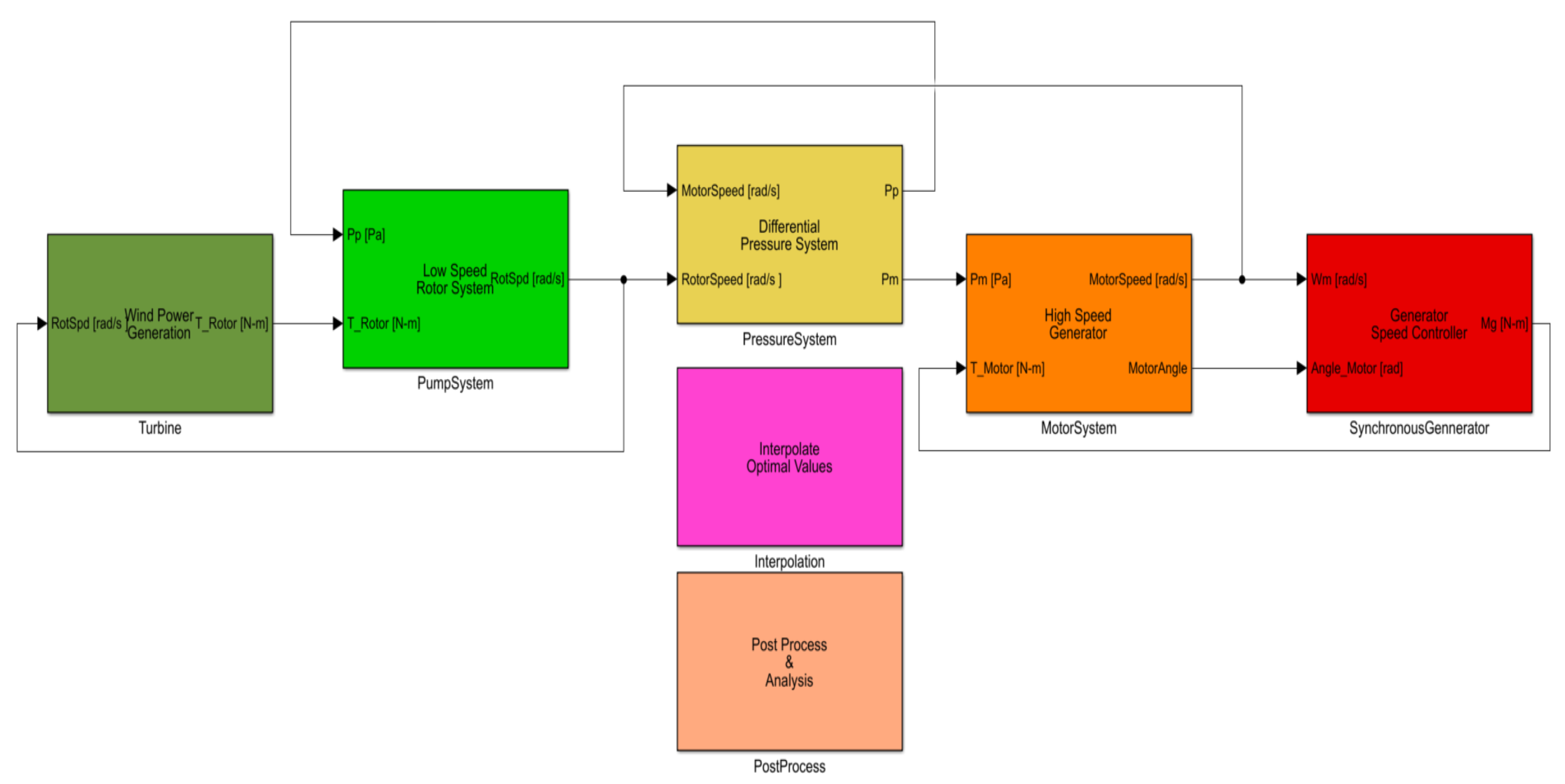
In this section, we present MPPT baseline simulation results. The dynamics of the Wind Turbine is designed in Matlab 2016b student version and is simulated for a 35 H NREL wind profile. The simulink block diagram of the wind turbine is shown in Figure 5.

The block Interpolate Optimal Values is not used in baseline simulation. It is only used for optimal reference generation for the control inputs in the proposed predictive controller.

Table 1. Wind Turbine Parameters.

Parameters	Symbols	Units	Value
Blade Radius	R	m	63
Blade Frontal Area	$\pi R^2$	m${}^2$	1.2469 × ${10}^4$
Air Density	$\rho$	kg/m${}^3$	1.225
Nominal Lambda	${\lambda }_i$	none	8.1
Nominal Rotor Efficiency	$C_p$	none	4.8
Power Coeff 1	$C_1$	-	0.5175
Power Coeff 2	$C_2$	-	116
Power Coeff 3	$C_3$	-	0.4
Power Coeff 4	$C_4$	-	5
Power Coeff 5	$C_5$	-	21
Power Coeff 6	$C_6$	-	0.0068
Max Efficiency	$C_{p_{Max}}$	-	0.48
Bulk Modulus	Pa	m	1.40403 × ${10}^9$
Pipe Diameter	$D_{Pipe}$	m	0.15
Pipe Length	$L_{Pipe}$	m	100
Pipe Volume	$C{h}_{Pipe}$	m${}^3$	1.7671
Cross-sectional Area	$A_{Pipe}$	m${}^2$	0.0177
Pipe Roughness	$R_{Pipe}$	m	1.5 × ${10}^{-5}$
Fluid Density	${\rho }_{fluid}$	Kg/m${}^3$	852.8
Fluid Kinematic Viscocity	${\nu }_{fluid}$	m${}^2/2$	18.786 × ${10}^{-6}$
Pump Inertia	$J_p$	Kg-m ${}^2$	38,759,228
Pump Mechanical Efficiency	${\eta }_{mec{h}_p}$	-	0.95
Pump Volumetric Efficiency	${\eta }_{vo{l}_p}$	-	0.95
Maximum Pump Volumetric Dispacement	$V_{p_{max}}$	m${}^3$/rad	0.3
Nominal Pump Speed	${\omega }_{p-nom}$	rad/s	1
Nominal Kinematic Viscosity	${\nu }_{p-nom}$	m${}^2$/s	18.876 ×${10}^{-6}$
Nominal Pump Pressure	$P_{p-nom}$	Pa	2 ×${10}^7$
Motor Inertia	$J_m$	Kg-m${}^2$	534.116
Motor Mechanical Efficiency	${\eta }_{mec{h}_m}$	-	0.95
Motor Volumetric Efficiency	${\eta }_{vo{l}_p}$	-	0.95
Maximum Motor Volumetric Disp	$V_{m_{max}}$	m${}^3$/rad	88
Nominal Motor Speed	${\omega }_{m_{nom}}$	rad/s	125.6637
Motor Fluid Kinematic Viscocity	${\nu }_{m_{nom}}$	m${}^2$/s	18.786 ×${10}^{-6}$
Genset Sync Speed	${\omega }_{m_{sync}}$	rad/s	125.6637
Sync Torque Coefficient	$K_S$	N-m/rad	$500\ast J_m$
Damping Torque Coefficient	$K_D$	N-m/(rad/s)	$20\ast J_m$

shows the nominal values of all the design parameters used in the design for simulation.

The wind data is not linearized and hence it has step change from wind speed to another and the dynamics see high speed switching in the synchronous generator. This causes a little spike in motor speed and hence with other signals within operational tolerance limits.

NREL Wind Data has a speed profile as shown in Figure 6. Baseline results which indicates the simulation performance of the dynamical system are shown in Figure 7, Figure 8, Figure 9 and Figure 10. These are the result from the system dynamics of the MATLAB simulink model as designed from the stated equations in the previous sections. The control action which is the pump and the motor displacements are based on the Pontryagin’s Minimum Principle based MPPT algorithm [3,4].

Figure 7 in particular shows the wind turbines performance in terms of its efficiency in capturing the wind power by the low moving blades and the final power capture by the high speed turbine to be supplied to the grids. The plot in GREEN is the actual power of the wind which is a direct function of the wind speed and the blade surface(swept) area. Now due to the pump capacity factor ($C_p$), which is maxed at a nominal value of $4.8$ the power at the rotor is almost halved, which is shown by the RED plot in Figure 7. The final power captured by the high speed motor is almost 80% of the power captured by the rotor which is shown by the BLUE plot in Figure 7. The two dashed rectangular boxes are the high wind speed regions where the maximum energy is harvested. Figure 8 shows the controlled high speed motor speed along with the optimal motor displacement as obtained by the Pontryagin’s Minimum Principle based Maximum Power Point Tracking (MPPT) algorithm. This optimal control is used for the baseline simulations as is published in literature [3,4]. The motor speed shows very good steady state behavior holding almost constant speed so as to generate electricity at the specified frequency. The load on the generator is adjusted by a simple Proportional/Derivative controller to maintain the generator speed at a constant RPM (125.63 rad/s) so that electricity is generated at rated frequency. The gains are applied to the motor speed and motor angle based on trial and error method which is shown in Figure 4.

Figure 9 shows the Pump Speed and Displacement plots. The optimal pump displacement is able to achieve quite a high degree of capacity factor. This will help to compare and understand the benefits when we look at the predictive controller results.

It is also observed and noted that a nominal value of 25 MPa for the transmission line pressure delta is achieved in baseline simulations. This pressure values are used as a constraint while solving for the predictive optimal problem. Figure 10 shows the base values of pump and turbine efficiency. $C_p$ is the Pump side efficiency or the capacity factor and $C_t$ is the efficiency on the high speed motor. The baseline optimal controller achieved a normalized capacity factor of close to 97% and the efficiency of the motor operation is around 88.5%. It is noted that the baseline non-predictive optimal controller performs quite well.

Later in the section Dynamic Programming based predictive controller will be evaluated and compared against these results to understand the benefits. Figure 11 shows the nominal values of the optimal pressure coefficients. The pressure coefficient states are initialized from a random initial value.

The optimal non-predictive controller which is based on the theory of Maximum Power Point Tracking using the Pontryagin’s Minimum Principle shows good performance under all wind speed regions. The motor speed tracking controller also indicates robust performance in maintaining steady state speed. Overall the baseline system as modelled based on published optimal control paper shows good metrics to compare against the proposed predictive controller results. In the next few sections the predictive controller structure will be discussed and the simulation results will be compared. All system constraints for the predictive optimal control problem is derived from the results obtained in the baseline optimal control.

3. Problem Formulation

The problem is formulated as a minimization problem to optimize the total system loss in the process. Minimizing total loss can be characterized as a maximization problem to increase efficiencies of Pump & Motor. Pump efficiency can attain a maximum value of 0.48 which is the nominal maximum capacity factor, for a nominal ${\lambda }_i$ of 8.1, which is a function, characterized by a polynomial fit between wind speed and blade pitch angle ($\beta$). Maximum value of Pump efficiency is obtained when the pitch angle ($\beta$) is 0.

The given optimal problem is formulated as a 5 states-2 controls problem with time being the other independent variable. The 5 states used in the admissible grid points are,

• Rotor Speed
• Differential Pressure
• Motor Speed
• Pump Flow Rae
• Motor Flow Rate

The objective cost is to maximize the pump and motor efficiencies together for a given set of control inputs at a given combination of state points. This is similar to discretizing the continuous time plant dynamics and then solving numerically for each discretized points to obtain the control parameters which maximises the cost function.

The inputs or the control factors are pump displacement and motor displacement in [m${}^3$/rad].

To maximize the efficiency we try to identify the losses in the system and how they can be minimized. There are two major loss components in the system, Aerodynamic loss & Hydro-static loss.

Aerodynamic efficiency which is directly co-related to the Aerodynamic loss is a direct measure of the Rotor Efficiency which indicates how much wind energy can be harvested by the rotor to be directly applied to the motor generator. The Aerodynamic loss can be defined as the difference between the actual tip-speed-ratio and the optimum tip-speed-ratio.

$$T_{s{r}_{opt}}-T_{s{r}_{act}}=T_{s{r}_{opt}}-\frac{R{\omega }_p}{V_{wind}}$$

(26)

The next big loss in the system is the hydro-static loss which is also known as the volumetric loss and is dependant on the pressure which is system state. Since viscous drag, coulomb friction and rotor/motor speed are functions of pressure the hydro-static loss can be formulated as:

$${\eta }_{tot-pump}=\frac{1-\frac{K_{S_p}}{A}}{1+A{C}_{vP}+C_{fP}},$$

(27)

$C_{vP}$ is viscous drag and $C_{fP}$ is Coulomb friction. $K_{S}p$ is pump slippage constant. A is a dimensionless factor which depends on the ratio of rotor speed and transmission line differential pressure: $A=\frac{\mu {\omega }_p}{P_{rs}}$ where $\mu$ is a system constant. Similarly for the motor, the loss can be termed as:

$${\eta }_{tot-mot}=\frac{1+\frac{C_1}{P_{rs}}+C_2}{1+C_3{P}_{rs}},$$

(28)

Hence using both the losses the the final efficiency can be attributed the below loss component:

$$h_{loss}=\frac{C_3{P}^2-C_2{P}_{rs}-C_1}{C_3{P}^2+P_{rs}}$$

(29)

Therefore combining the Aerodynamic loss and the the hydro-static loss component a final detailed performance index can be derived as [3,4,13]:

$$\begin{array}{cc}\hfill J^{*}\left(t\right)& ={\int }_{t_0}^T[{\alpha }_1{(T_{s{r}_{opt}}-\frac{R{\omega }_p}{V_{wind}})}^2\hfill \\ & +{\alpha }_2\left(\frac{C^3{P}_{rs}^2-C_2{P}_{rs}-C_1}{C_3{P}_{rs}^2+P_{rs}}\right)]\mathit{dt}\hfill \end{array}$$

(30)

where, $C_1$, $C_2$ & $C_3$ are pressure dependent constants, $J^{*}\left(t\right)$ is the accumulated cost-to-go for the entire prediction window starting from the end of the window.

The above equations states the two major contributors of losses in the system, one at the rotor and the other at the motor. Effectively reducing the losses means increasing the efficiencies of the rotor and the motor. Hence a reduced order cost function can be thought of in terms of the efficiencies. Since it is challenging to increase both the efficiencies in the same magnitude and tunable parameter ($\alpha$) is designed in order to adjust between the low speed rotor efficiency and the high speed motor efficiency. Hence the final computational ready performance index is reduced in terms of efficiencies, such as:

$$J^{*}\left(t\right)={\int }_{t_0}^T-[{\alpha }_1{c}_{rotor}+(1-{\alpha }_1)c_{motor}]\mathit{dt}$$

(31)

where, $c_{pump}$ & $c_{motor}$ are the respective rotor & motor efficiencies, $J^{*}\left(t\right)$ is the accumulated cost-to-go for the entire prediction window starting from the end of the window.

The negative sign before the integrand is due to the fact that minimizing losses is similar to maximizing efficiency.

Finally the individual constraints are applied on the states and controls to keep the dynamics within physical possible limits of operation. Constraints are applied in the form of high penalty to the cost function when they are violated.Typical constraints for this formulation are on Differential pressure ($P_{rs}$) less than 0 or going negative, motor speed (${\omega }_m$)too transient and rotor speed (${\omega }_p$) within certain tolerable zone.

4. Dynamic Programming Background

Once the performance measure of the system or the cost function is determined the next major task is to define a control function that would minimize the performance criteria.

Two widespread methodology to accomplish this task are minimum principle of Pontryagin and the method of Dynamic Programming. Pontryagin’s minimum principle is a variational approach that lead to a non-linear two point boundary value problem which is solved to get the optimal control.

Dynamic Programming (DP) is both a controls methodology and a computer programming method to numerically solve an optimization problem given a set of admissible controls and state space grid vectors. It always satisfies global optimality as it finds the minimum value of the cost/objective function from all admissible search space. Since it has to traverse a full factorial design of experiment (DOE) of search space for all the controls & states it is often challenged by the curse of dimensionality [14]. The next two sections discusses the principle of optimality and describes the step wise procedure for dynamic programming algorithm.

4.1. Principal of Optimality

In controls literature a general control law is defined by Equation (32),

$$u_i^{*}\left(t\right)=f(x_i\left(t\right),t)$$

(32)

where, $u_i^{*}$ is the optimal control effort, $x_i\left(t\right)$ are the states of the system. which is a closed loop or feedback optimal control. The functional relationship f is called the optimal control law or optimal policy. The control law specifies how to generate the control law from the states at a given time, since this is a time varying control formulation. Dynamic programming specifically solve the controls problem applying the principle of optimality.

Bellman’s original Optimality Principle, states:

An optimal policy has the property that whatever the initial state and initial decisions are, the remaining decision must constitute an optimal policy with regard to the state resulting from the first decision. In Figure 12, if $J_{abe}$ is the minimum cost to go from a-e, then from b-e the minimum cost has to be $J_{be}$ and $J_{bce}$ cannot be the optimal path.

That is $J_{bce}>J_{be}$.

Dynamic programming is based on the same principle to find the optimum cost at each time step traversing backwards and then figuring out the optimal cost to go in the forward simulation which by the principle of optimality is claimed to the global optimal result.

Figure 13 depicts such a condition of admissible control selection. An alternative notation for the computational formulation of the dynamic program algorithm is shown in Equation (33)

$$\begin{array}{cc}\hfill J_K^{*}\left(x(N-K)\right)& =\underset{\mathit{u}(\mathit{N}-\mathit{K})}{min}[g_D(x(N-K),u(N-K))\hfill \\ & +J_{K-1}^{*}(a_{D}x(N-K),u(N-K))]\hfill \end{array}$$

(33)

with, K being each stage during the search process and $J^{*}$ is calculated for each stage K, which is known as stage cost. N is the total number of discretized stages. $g_D$ & $a_D$ comes from the definition of the system model dynamics which can be ignored in this section. This in general illustrates that each stage the stage cost is calculated and is added on to the over all cost which is known as the cost-to-go and this cost-to-go is used for the forward simulation. This is a general design of objective cost function used by dynamic programming. This is not the cost function which is solved for the proposed controller in this paper.

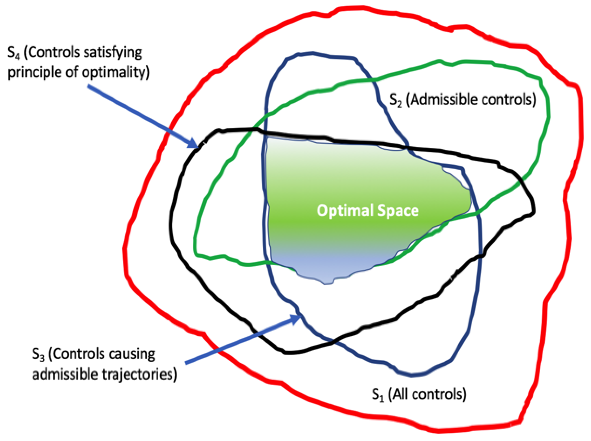
Since a direct search is used to solve the functional recurrence equation, the solution obtained is absolute (or global) minimum. Dynamic programming makes the direct search feasible because instead of searching among the set of all admissible that cause admissible trajectories, we consider only those controls that satisfy additional necessary condition—principle of optimality.

4.2. Dynamic Program Algorithm

Dynamic programming algorithm involves a complex and computationally challenging process which is described below.

• Baseline Run: Simulate the baseline plant to store results for comparison and gather data for dynamic program initialization
• Feasible Grid Search: This step is the most time consuming and computation heavy process. It loops through all the combinations of feasible grid points for states & controls, then store the next iterated value for each state & cost/performance metric parameters.
• Optimal Control Selection: This step is heart of dynamic programming where the minimum stage cost is calculated and the optimal cost-to-go is selected from the minimum stage cost. The corresponding minimum controls value for each optimal stage cost is also selected.
• Simulate Optimal Controls: The final step is to apply the optimal controls generated in the previous step to see the final outcome of the dynamical plant. The optimal controls is selected based on interpolated n-D look up tables since it is a function of the number of states and the independent time vector. Figure 14 shows the interpolation method used to select the optimal pump/motor displacements and the cost-to-go at each step.

Interpolation of the n-dimensional search space is done to select the optimal control values and the cost-to-go. It is required to do the interpolation since while going forward in simulation it is not necessary that the states coincide exactly with the grid points.

Figure 14 shows the propagation of state variables in every time step. The green paths at each time instant shows the possible path that the state can take but the red paths are the one which are the interpolated optimal path.

Table 2. Dynamic Programming Grid Setup.

Parameters	States	Controls	Units	Grid Points
Rotor Speed	Yes	No	rad/s	17
Differential Pressure	Yes	No	Pa	10
Motor Speed	Yes	No	rad/s	5
Pump Flow Rate	Yes	No	m${}^3$/s	5
Motor Flow Rate	Yes	No	m${}^3$/s	5
Pump Displacement	No	Yes	m${}^3$/rad	10
Motor Displacement	No	Yes	m${}^3$/rad	10

shows the discretized grid setup for the states and control variables. The grids are chosen such that the dynamics are still captured between the step size and the grid is not too large to challenge the computational cost. The grid size is decided based on the observed dynamics from the baseline optimal controller.

5. Optimal Control Strategy

The proposed dynamics of the wind turbine is modelled to be optimized with Dynamic Programming as described in the previous sections. In Figure 15, it is noted that the high level power profiles look very similar to the baseline optimal control results. It may be noted here that the wind power is same as the baseline wind power wind power since the wind power cannot change. The regions where the benefits come in the proposed predictive controller is during the high wind speed regions which is highlighted by the red dashed rectangles. It is also observed that the Rotor Speed & hence the efficiency is reduced during a sudden decrease in wind speed level at certain section of the wind profile. This is also sometimes the reason why there is a cut off limit for wind speed both on the high and low side to operate the turbine. We also see that the high speed switching spikes is there but with negligible effect to the optimization study.

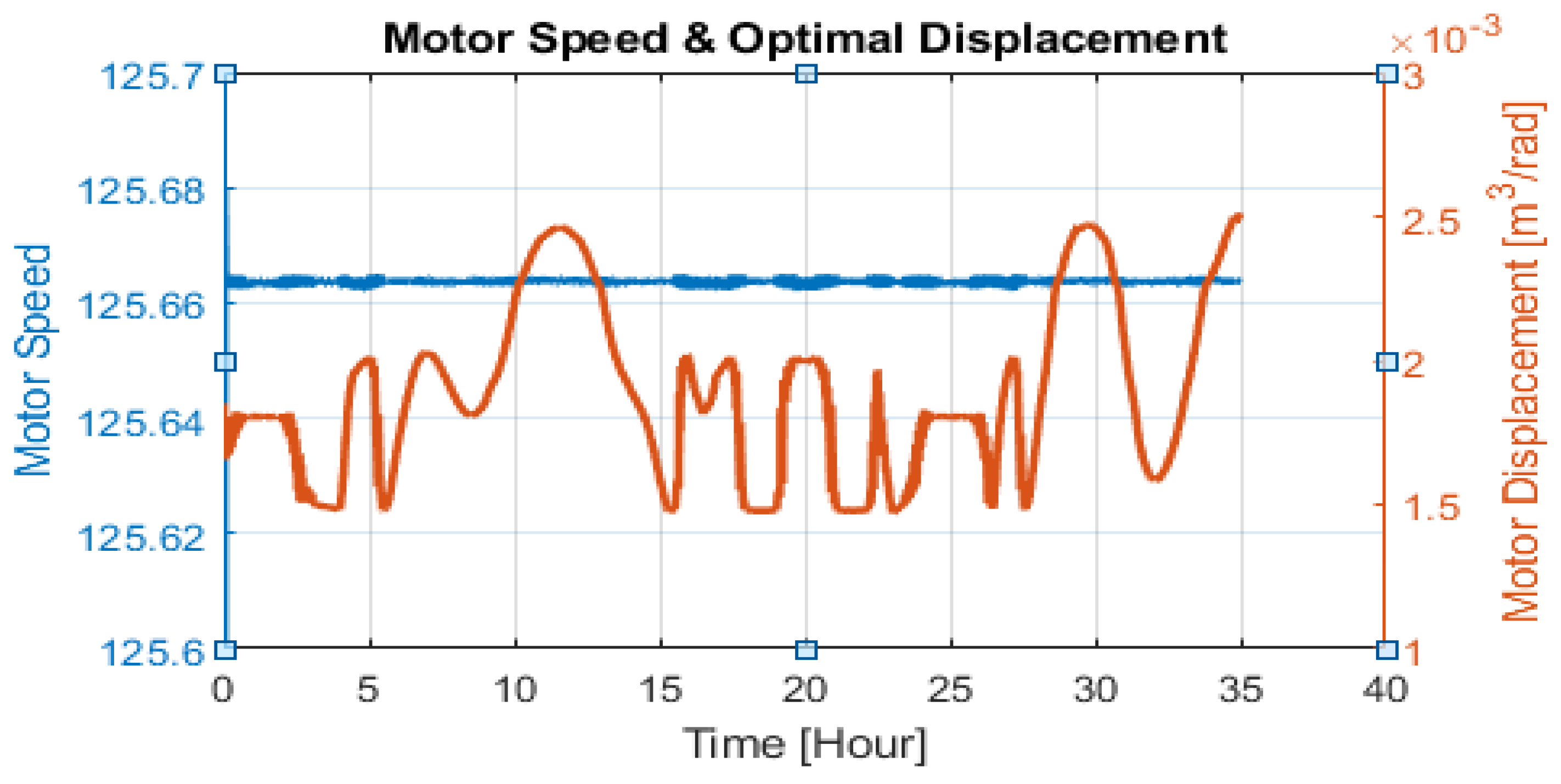
Figure 16 and Figure 17 shows the optimal control levers along with the respective rotor speed and motor speed. The results shows that the control actuation obeys constraints and there is not much oscillations in the control action. It is important to note that motor speed (${\omega }_m$) is very close to the operating synchronous generator speed for power generation at 60 Hz. We do see very minor spikes in the motor speed and that is because of high speed switching during a step change in the wind speed. The results indicate that it is hard to optimally capture the wind energy at low speeds and the optimal wind speed zone is close 12–14 m/s.

It is also worthwhile to note in Figure 17, that with the optimal control entitlement using Dynamic Programming the synchronous generator proportional plus derivative control does a good job of adjusting the load controller to maintain the motor speed within required specification for power generation at fixed supply line frequency.

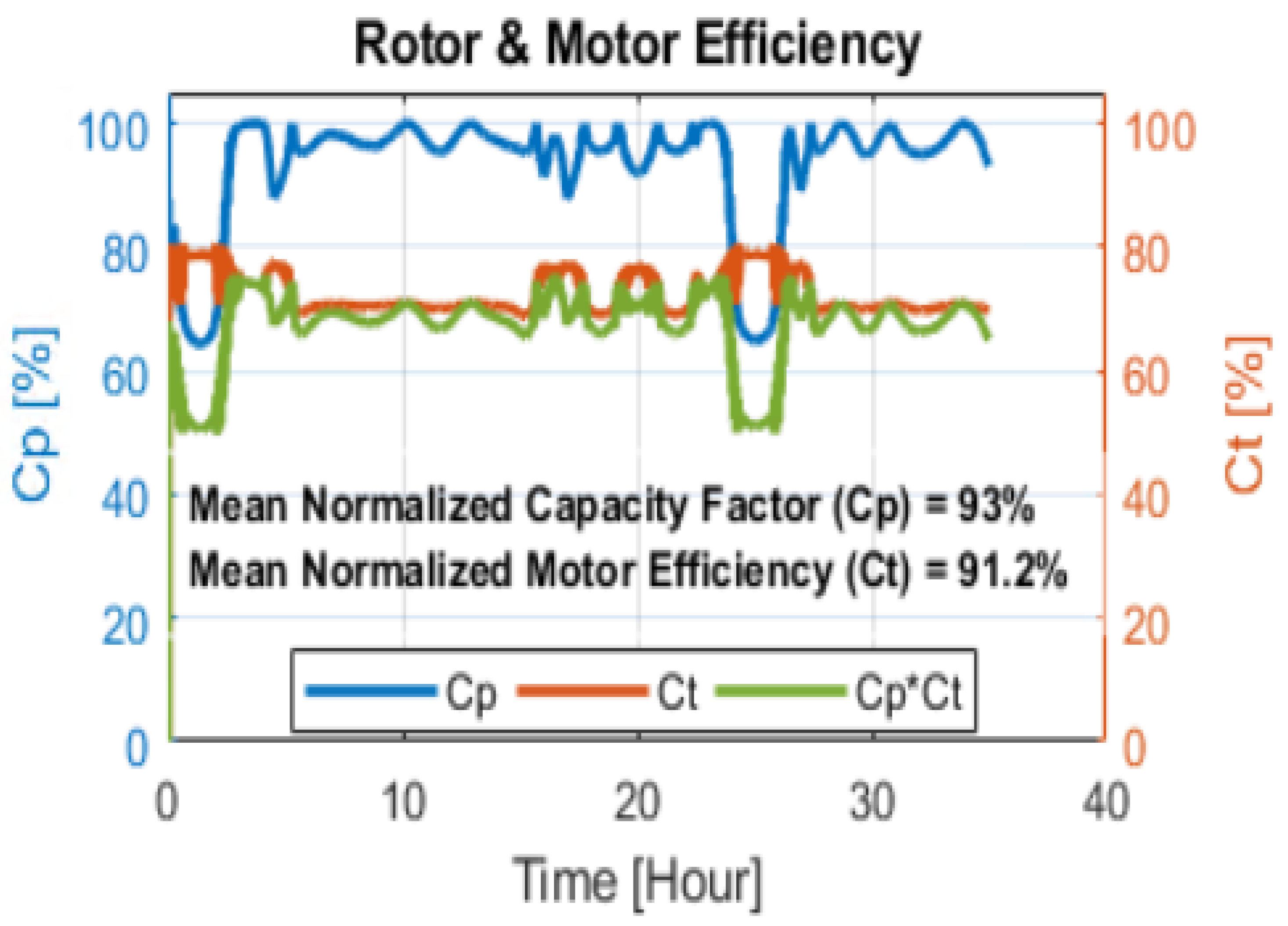
Figure 18 shows the individual efficiencies of the low speed pump and high speed turbine. It shows that knowing the wind profile in advance can better help to optimize the pump and motor displacements in m${}^3$/rad so that less actuation energy is utilized while capturing maximum power possible. Definitely the control rule has to be created which is a function of the wind speed as shown by the entitlement using dynamic programming. Since Dynamic programming is a global optimal solver within the admissible control/state space we conclude that this shall be the best optimal control. It is observed that a reduction in Pump Capacity factor took place with the predictive controller. The pump capacity factor is 93%. There is an increase in the high speed motor efficiency which went up to 91.2%.

It also shows that at certain section of the wind speed it is very difficult to capture the maximum available power which is also very obvious for transients in wind speed. We also saw some high speed switching glitches in motor speed but the Proportional-Derivative control permanent magnet synchronous generator (PMSG) control designed is well handling the situation and thereby keeping the variation in motor speed well within specifications.

Figure 19 shows the energy differences between the baseline optimal controller which is the Maximum Power Point Tracking algorithm and the Look Ahead based optimal strategy as discussed in this paper. It shows that the look ahead knowledge of the wind speed helps to achieve a 4 MWh of more energy harvest. This is a 3.5% increase over the baseline optimal controller. Looking at the power profile we notice that the maximum benefit of the look ahead based controller is achieved during the high wind speed zones. Figure 20 illustrates the benefits of the proposed predictive controller in terms of the energy captured in the form of a bar chart. It is observed that the proposed controller can achieve a $3.6\%$ better energy capture over a time period of 35 h. This is solely based on the look ahead knowledge of the wind speed over the entire duration of the cycle. It is also noted that the major benefits occurred during the high speed wind regions. It is also worth pointing out that the performance of the proposed controller is worse than the baseline optimal controller. It is observed that the new controller efficiency is almost half as the baseline controller during the low wind speed regions. This did not affect the results since at low wind speeds the power capture is extremely low and so overall there is no substantial gain in energy harvest. Hence the new proposed controller optimized the control effort knowing that it will have better wind speed regions to harvest more energy over the entire wind profile.

Figure 21 shows the optimized differential pressure in the hydraulic lines. It is observed that there are some high frequency noise within tolerable band due to the high speed switching in wind speed. The optimal problem also has a constrained setup for this state which is to restrict the pressure between 5 & 30 MPa and the plot shows that the constraint is well followed and also within system limits. A high value of around 24 MPa is achieved during a very high wind speed. These are the regions where maximum energy conversion is achieved.

Figure 22 shows the optimal pressure coefficients. As a last step, we analyzed the optimal controller performance when we do not have accurate prediction of the wind speed. To do this we introduced 2%, 5% and 20% inaccuracies in the prediction of the wind speed both on the positive and negative side. The inaccuracy is introduced as a constant offset to the actual wind speed. Figure 23, shows the performance of the controller for different inaccuracy levels. It is observed that a 2% inaccurate wind speed prediction does not change the result significantly. When we introduced inaccuracies of the order of 5% we see that if the prediction is inaccurate by positive offset (which means the predicted wind speed is 5% more than the actual wind speed), there is a loss in energy capture. However when we introduced the inaccuracy in the negative side we see an increase in the energy capture. This indicates that if we predicted the wind speed by 5% less than the actual value it provides better benefits. 20% inaccuracy is not at all suitable for predictive control, which in other words means if the prediction is not very accurate then it will not bring in true benefit.

6. Conclusions and Future Work

We presented a predictive look ahead knowledge based control methodology for a hydro-static drive wind turbine that optimizes the overall efficiencies under varying wind speed. The proposed control strategy optimally selects the control variables (Pump & Motor Displacements) more efficiently with less control actuation effort. Dynamic programming which is based on the well established principles of Hamilton-Jacobi-Bellman, chose global optimal values for the control parameters with the objective of minimizing the overall losses. The results of the proposed controller is compared against published literature based on Pontryagin’s Minimum Principle optimization algorithm for maximum power point tracking. It is observed that having a predictive controller can provide around 3.5% better performance in terms of improving total system losses and harvesting energy over MPPT. It is not always feasible to implement a complex numerical method such as dynamic programming, in embedded systems, so a rule based control often needs to be designed based on the analysis of the outcome of the dynamic programming results. The simulation results show that the proposed look-ahead strategy offered optimal operation of the wind turbine by closely tracking the optimal tip-speed ratio to maximize capacity factor while maintaining the hydraulic motor speed close to the desired value to ensure that the frequency of electrical output is nearly constant. This study indicates that there is potential in including look ahead information in optimal control design for a hydro-static drive wind turbine.