
Influence of Injection Well Location on CO2 Geological Storage Efficiency


Division of Geotechnology, Mineral and Energy Economy Research Institute of the Polish Academy of Sciences, 31-261 Kraków, Poland
Energies 2021, 14(24), 8604; https://doi.org/10.3390/en14248604
Submission received: 21 September 2021
/
Revised: 24 November 2021
/
Accepted: 15 December 2021
/
Published: 20 December 2021
(This article belongs to the Topic Carbon Capture, Storage and Utilisation Technologies (CCS/CCU))
Abstract
:An analysis of the influence of injection well location on CO2 storage efficiency was carried out for three well-known geological structures (traps) in deep aquifers of the Lower Jurassic Polish Lowlands. Geological models of the structures were used to simulate CO2 injection at fifty different injection well locations. A computer simulation showed that the dynamic CO2 storage capacity varies depending on the injection well location. It was found that the CO2 storage efficiency for structures with good reservoir properties increases with increasing distance of the injection well from the top of the structure and with increasing depth difference to the top of the structure. The opposite is true for a structure with poor reservoir properties. As the quality of the petrophysical reservoir parameters (porosity and permeability) improves, the location of the injection well becomes more important when assessing the CO2 storage efficiency. Maps of dynamic CO2 storage capacity and CO2 storage efficiency are interesting tools to determine the best location of a carbon dioxide injection well in terms of gas storage capacity.
1. Introduction
The concept of mitigating climate change using underground carbon dioxide storage technologies has attracted increasing attention in recent years. Identifying potential geological structures for underground CO2 storage and developing a methodology to estimate their capacity are essential elements that will determine the effectiveness of their application [1,2].
1.1. Capacity of Geological Structures for CO2 Storage
Estimates of CO2 storage capacity are made at different scales depending on the needs. They may refer to a country, basin, region, or a specific recognized geological structure. The estimation of theoretical CO2 storage capacity is based on calculating volumetric capacity and available pore volume. Several methods for the volumetric estimation of CO2 storage capacity in deep aquifers are presented in the literature [3,4,5,6]. It is possible to calculate the capacity as the mass of the stored CO2 while considering carbon dioxide density in reservoir pressure and temperature conditions [7]. For the calculations performed in this article, the CSLF method proposed by the Carbon Sequestration Leadership Forum was chosen. In this method, the estimation of the amount of CO2 stored in the geological trap is based on calculating the volume of stored CO2 depending on the geometric volume of the trap, porosity, the irreducible water saturation, and the CO2 density in reservoir conditions.
The generalized equation presented in the CSLF method was used to estimate the theoretical storage capacity of the Konary, Sierpc and Suliszewo structures [5,7,8,9]:
where:
—CO2 storage capacity calculated by the CSLF method, [kg],
—average CO2 density under given pressure and temperature conditions, [kg/m3],
—area of the structure (trap), [m2],
—average thickness of the structure (trap), [m],
—average porosity of the structure (trap), [-],
—irreducible water saturation, [-].
1.2. CO2 Storage Efficiency
The CO2 storage efficiency is understood as a fraction of the reservoir pore space volume that can be filled with CO2. In addition to the petrophysical properties of the rocks, it is influenced by: the geometry of the structure, the stratigraphic heterogeneity of the reservoir, the hydrogeological parameters of the reservoir, and other additional factors such as the number of injection wells, their location, and requirements related to the safety of the storage process [9]. The quality of the sealing and the geological structure of the reservoir are other important factors affecting the storage efficiency [10]. Their influence is difficult to estimate without detailed studies, including carbon dioxide injection simulations [11].
Bradshaw et al. [12] introduced the concept of primary CO2 storage capacity, understood as the total pore volume of the reservoir of the carbon dioxide storage structure. This volume is not likely to be filled with carbon dioxide. Therefore, the concept of storage efficiency, which is the ratio between the maximum storage volume and the actual injected volume, was introduced [13]. Depending on the aquifer hydrogeological parameters and the type of storage, storage efficiency is usually estimated between 2 and 17% [12,13,14].
The CSLF method for estimating the storage capacity of CO2 assumes that the value of the storage efficiency depends on whether the structure being considered for storage is a closed, partially closed, or open structure and on the quality of the reservoir petrophysical properties (porosity and permeability). A porosity above 20% and permeability above 300 mD are considered as good petrophysical properties [15,16], although other sources state that the porosity above 15% and permeability above 100 mD are required [17]. A porosity lower than 10% and permeability lower than 100 mD are considered poor petrophysical properties of the reservoir [16]. For structures where the trap and the aquifer are connected, the storage efficiency is 40% for structures with good reservoir parameters and 20% for structures with poor reservoir parameters. For partially closed structures, the storage efficiency is 10–20% for a reservoir with good quality and 5–10% for a reservoir with poor quality. For closed structures, this efficiency ranges from less than 3% for reservoirs with poor quality to 3–5% for reservoirs with good quality [15,18].
Vangkilde-Pedersen et al. [19] used the modified CSLF method to estimate CO2 storage capacity. They assumed a storage efficiency of 3–40% for open and semi-enclosed structures and 1–20% for enclosed structures. The latest CSLF report [20] shows that the storage efficiency, the proportion of pore space utilized, is very low. In the case of saline formations, CO2 storage efficiency represents 1–4% of the bulk volume (with 15–85% confidence).
The US DOE (United States Department of Energy) method is similar to the CSLF method of calculating CO2 storage capacity. The difference between them is that the expression with irreducible water saturation (1-Swirr) in the CSLF method is included in the main formula for calculating capacity. In contrast, the US DOE method is included in the storage efficiency factor. So, if we multiply the efficiency by (1-Swirr), we get a correspondingly reduced CO2 storage efficiency for the US DOE method. For example, Goodman et al. [6] found that, for the US DOE method, the efficiency for saline formations ranges from 0.40 to 5.5% for the three different lithologies over the 10 and 90 percent probability ranges.
1.3. Dynamic Storage Capacity
The most critical geomechanical parameters that determine the safety of storage are fracture pressure and capillary entry pressure (the critical pressure when supercritical CO2 “breaks” through the capillaries of the overlying seal) [16]. The capacity calculated using analytical modeling or numerical simulations, considering the mentioned parameters, is called dynamic capacity [9]. Van der Meer and Egberts [21] and van der Meer and Yavuz [22] drew attention to the fact that the very act of injecting CO2 into the aquifer causes an increase in pressure that can limit its capacity if permissible levels are exceeded.
The estimation of the dynamic storage capacity of CO2 takes into account such parameters as the allowable pressure increase in the structure due to injection, the number and location of gas injection wells, and the injection time. It is also essential that the CO2 does not exceed the spill point. This means that the injected CO2 does not exceed the defined structural boundary as a result the movement within the rock pores due to the pressure changes caused by the gas injection. The dynamic CO2 storage capacity is estimated by simulating the CO2 injection using reservoir simulation.
1.4. Previous Studies on CO2 Storage Capacity in Poland
The CO2 storage capacity in Poland has been the subject of several recent publications. Uliasz-Misiak [14] estimated storage capacity (theoretical, effective, and practical) for the most promising aquifers in Poland using a simplified methodology considering average porosity values, the average fraction of permeable layers, average CO2 density under reservoir conditions, and the storage efficiency. The effective and practical storage capacity was determined for three different storage efficiencies (1, 4, and 8%). Based on computer simulation, the author presented estimates of dynamic CO2 storage capacity for a selected aquifer (with efficiencies of 10, 20, and 40%) and compared the obtained results with estimates of theoretical storage capacity. Tarkowski [23] presented the results of the capacity estimations (volumetric and dissolution) for 48 structures located in the Mesozoic saline horizons of the Polish Lowlands with the assumed storage efficiency of 20%.
Within the framework of the EU GeoCapacity project, the CO2 storage capacity (resulting from structural trapping) was estimated (according to the methodology proposed in the EU GeoCapacity project) for the selected deep Mesozoic aquifers in Poland [24,25,26]. The CO2 storage capacity for the Mesozoic reservoirs of the Polish Lowlands was estimated: for the Lower Cretaceous—7647 Mt, Lower Jurassic—43,826 Mt, Lower Triassic—26,494 Mt, and for 18 selected geological structures—3522 Mt. The results showed that the storage of CO2 in the Mesozoic aquifers of the Polish Lowlands is the best possible option for the geological storage of this gas due to its large capacity [25]. Marek et al. [27] estimated the volumetric CO2 storage capacity of the Zaosie structure to be 340 Mt of CO2, with a storage efficiency of 10%. Tarkowski et al. [28] characterized in detail selected potential structures for CO2 storage in the Mesozoic formations of the Szczecin-Mogilno-Uniejów Trough and evaluated their usability and capacity for underground carbon dioxide storage. The Konary structure was characterized in terms of CO2 storage and based on the CO2 injection simulation, and the CO2 storage capacity for the Lower Jurassic was estimated [29,30]. Different locations of the CO2 injection well in the Konary structure, considering the capillary entry pressure of the caprock, [30] showed that the consideration of the capillary entry pressure at the top of the structure resulted in a significant reduction of the dynamic capacity by up to 60%. For selected aquifers in the Bełchatów region, Labus et al. [31] estimated the CO2 storage capacity by dissolution at 11.1 kg/m3 of the formation, while, for the Jurassic sandstones from the Chabowo anticline, the dissolution capacity was estimated between 9.19 and 12.0 kg/m3 [32].
1.5. Research Objective
The effect of the CO2 injection well location within the geological structure on the CO2 dynamic storage capacity, and further on the value of CO2 storage efficiency, is a crucial issue that has not been fully addressed in the literature. However, Stopa et al. [33] developed computational methods to optimize the location of the injection well for a different purpose, namely, to minimize the risk of CO2 leakage. Hajiabadi et al. [34] also emphasized that most models have focused on reservoir-level CO2 storage capacity rather than well injectivity and attempted to identify the gaps by examining the significant factors contributing to CO2 injectivity in deep saline aquifers. In turn, Okwen et al. [35] performed numerical simulations of CO2 injection to evaluate the gas storage efficiency for different sedimentation environments at five different CO2 injection well locations. It allowed them to find the difference in the magnitude of this efficiency for other well locations. However, this is another important issue that has not been substantially investigated, as only the average value of the results obtained at five CO2 injection well locations was calculated. Hu et al. [36] also noticed a difference in CO2 storage capacity due to the location of the injection well, although they studied storage at an oilfield. Jun et al. [37] analyzed four well patterns to define the optimal injection well pattern, placement, and operating conditions. The results showed the optimal location and fluid rate that enabled an almost eight times larger volume of CO2 to be stored compared to the base case. Urych and Smoliński [38] considered several simulation variants of CO2 injection into geological formations and determined the best reservoir for potential geological storage of CO2 from the three studied reservoirs, characterized by the most favorable geological and hydrogeological parameters. White [39] found that CO2 static capacity estimates from well-based mean values are less than comparable seismic-based estimates by <15% due to porosity differences and by <5% due to thickness differences. Variations in thickness of up to 25 m from the mean value could result in capacity estimate differences of up to 25% for alternate well locations.
In the present article, the research objective is to show the influence of the CO2 injection well location on the storage efficiency of the considered geological structure. For this purpose, three geological structures from the area of the Polish Lowlands were selected and characterized, assuming CO2 storage in Lower Jurassic aquifers. A set of theoretical and dynamic CO2 storage capacities for each of the selected structures was obtained by simulating CO2 injection with fifty different injection well locations to assess how storage efficiency depends on the injection well located concerning various geological structures.
2. Materials and Methods
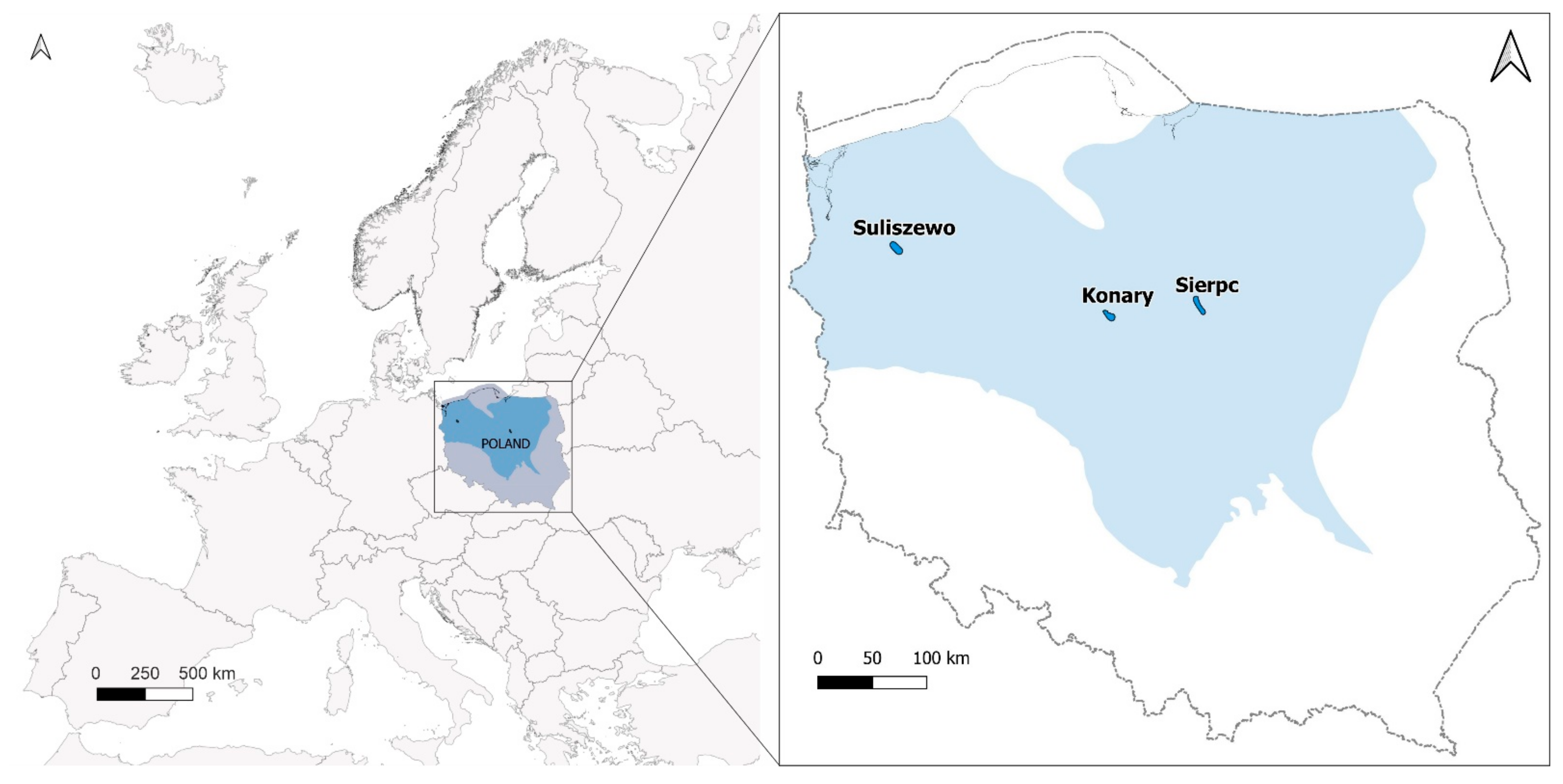
Three selected geological structures for CO2 storage in deep aquifers of the Lower Jurassic (Komorowo Beds or their equivalent), representing three different geological units of the Polish Lowlands, were analyzed in detail: the Konary anticline (Pomeranian-Kuyavian Swell), Sierpc anticline (Marginal Trough), and Suliszewo anticline (Szczecin-Łódź Trough) (Figure 1).
These structures were selected based on the availability of detailed geophysical data and their position in the geological structures of the Polish Lowlands ranking presented by Uliasz-Misiak and Tarkowski [40].
Spatial geological models were created for the Konary, Sierpc, and Suliszewo structures, and numerical modeling of CO2 injection was performed. The dynamic storage capacity was estimated separately for each structure and fifty CO2 injection well locations. The CO2 storage efficiency was then determined based on the dynamic storage capacity and the calculated theoretical storage capacity.
2.1. Geological Characteristics of the Considered Structures
The detailed geological characteristics of the considered structures were presented by Marek et al. [41] and supplemented with the results of well geophysical surveys (natural gamma-ray profiling, standard resistivity profiling) to determine the porosity and permeability of the reservoir rocks [42]. In recent years, the Konary structure has been examined in detail to assess the influence of the reservoir parameters [29] and cap rock capillary entry pressure [30] on the estimation of CO2 storage capacity. The Suliszewo structure was analyzed in the context of its use for hydrogen storage [43]. The Sierpc structure was also described to estimate and compare CO2 storage capacity and H2 storage capacity [44]. The data assumed for CO2 injection modeling concerning the analyzed structures are presented in Table 1.
2.1.1. Konary Structure
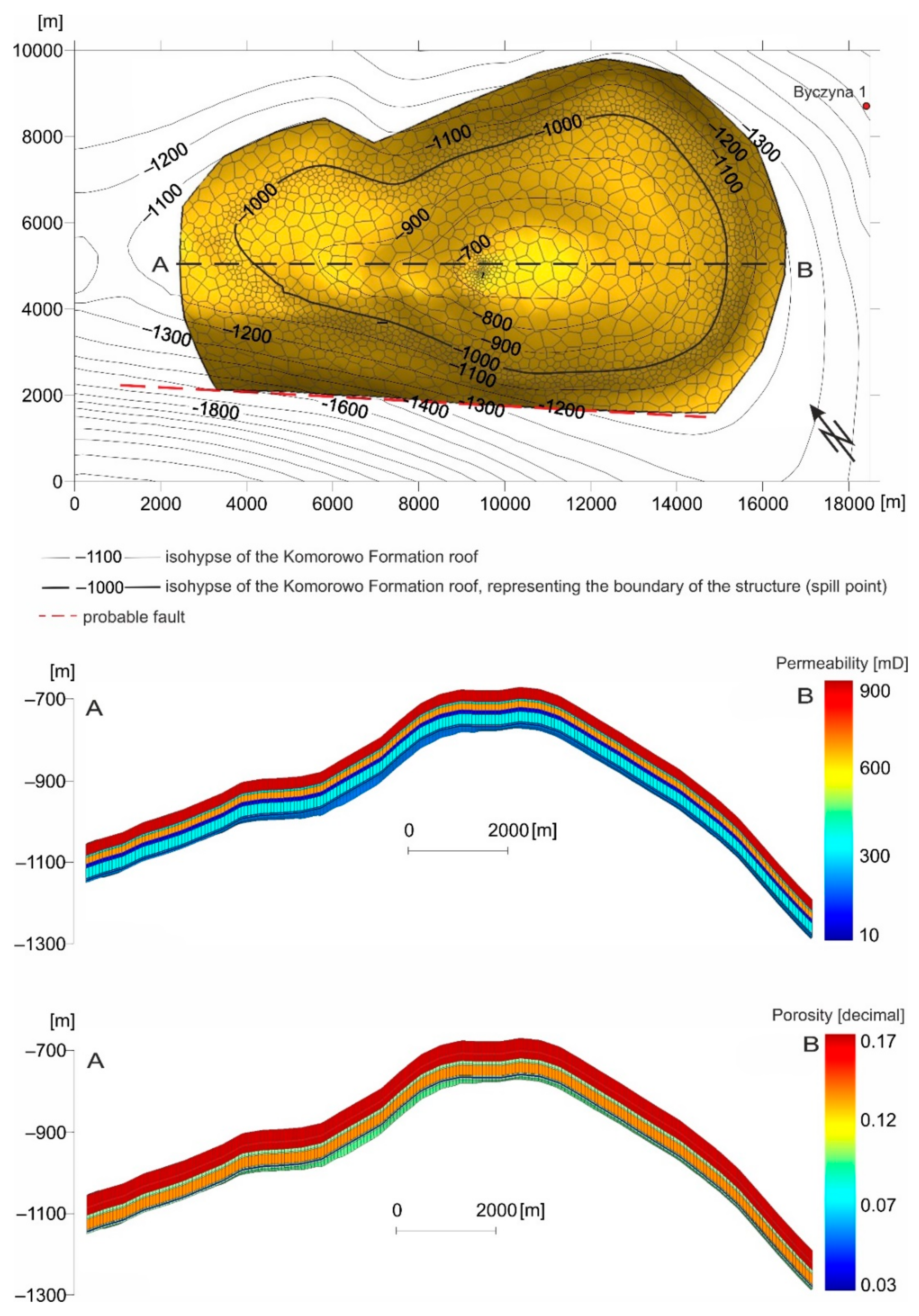
The Konary anticline was identified by a semi-detailed image of a reflection seismic survey and two wells: Konary IG-1, with a final depth of 3452.0 m (Zechstein) on the NE-wing, [45] and the research well Byczyna 1, with a final depth of 5728.0 m (Carbon Lower) on the SE-wing of the structure. The lithostratigraphic and hydrogeological analysis of the Mesozoic deposits of the Konary anticline showed that the upper Komorowo Formation of the Upper Pliensbachian reservoir is the most favorable for CO2 storage [46]. It was drilled in the Byczyna 1 well at 1832.0–1926.0 m (thickness 94 m). The Komorowo Formation in the upper part of the profile is represented by fine-, medium-, and coarse-grained sandstones with very good reservoir properties, with a maximum permeability of 1000 mD (average 900 mD) and a maximum porosity of up to 18% (average 16.75%). A higher proportion of claystones characterizes the lower part of the profile of this formation. The rocks of this formation are filled with class I calcium chloride brines with mineralization of 42–49 kg/m3 [47,48]. The Komorowo sandstone formation is sealed from above by clay and silt layers with thin inserts of fine-grained sandstones, sometimes with a calcareous-dolomitic or sideritic binder, with an average thickness of 125 m, contained to the Ciechocinek Formation of the Lower Toarcian. It was assumed that the elliptical-oval outline (spill point) of the anticline was determined by the Upper Jurassic Pliensbachian roof isohypse of −1000 m [41].
2.1.2. Sierpc Structure
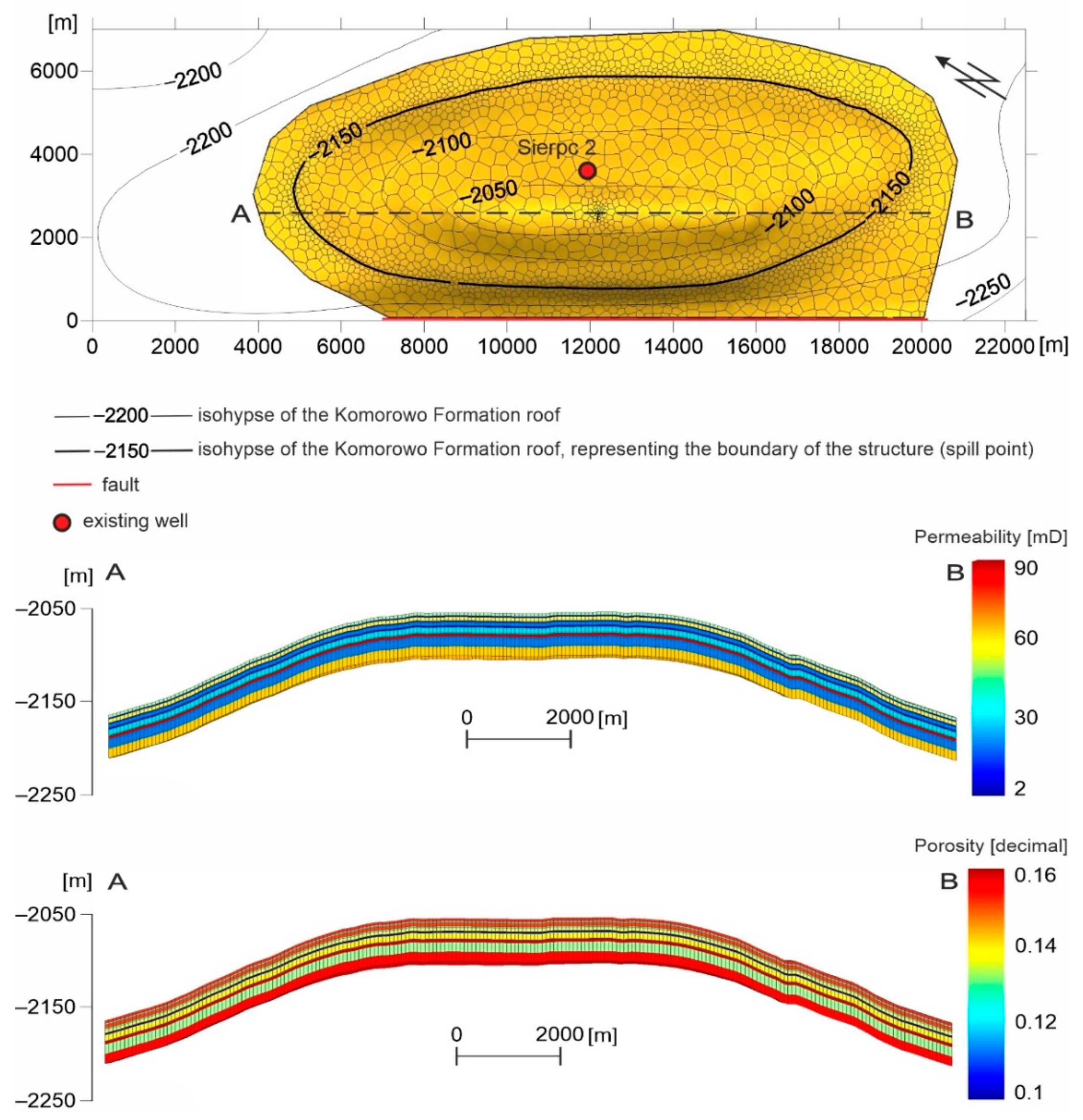
The Sierpc anticline was recognized by a regional image of a seismic reflection survey and two deep wells, Sierpc 1 (2100.5—Lower Jurassic, Lower Toarcian) and Sierpc 2 (4389.0 m—Carbon), located at the culmination of the structure. The selected Lower Jurassic reservoir [49,50,51] was drilled in the Sierpc 2 well at a depth of 2190.0–2236.0 (46 m). This level consists of fine and medium-grained light gray sandstones with an average permeability of 50 mD and an average porosity of 15% and clay-silt interbeds with an average permeability of 2 mD and an average porosity of 10%. This level includes Class I chloride-calcium brines with a mineralization of 100–200 kg/m3. The claystone Ciechocinek formation seals the reservoir of the Drzewice Formation. It was drilled in the Sierpc 2 well at 2112.0–2190.0 (78 m). It consists of clay and silt deposits with thin sandy interfaces, concretions, and iron streaks. The petrophysical properties of these formation rocks confirm their sealing ability [51]. It is assumed that the elliptical-oval outline (spill point) of the anticline was determined by the Lower Jurassic isohypse of the Upper Pliensbachian roof with a value of −2150 m.
2.1.3. Suliszewo Structure
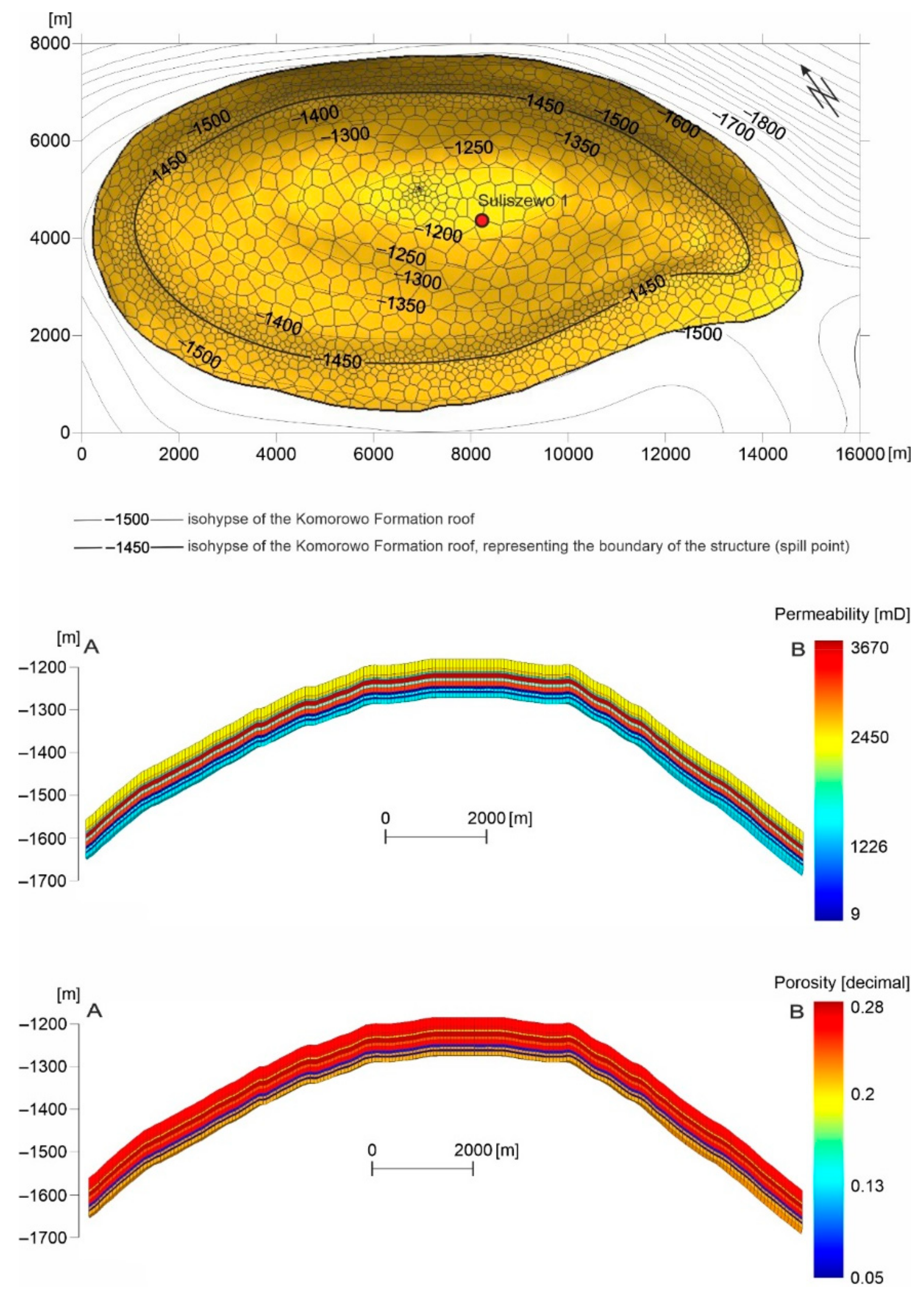
The Suliszewo anticline was identified by a semi-detailed image of a seismic reflection survey and the Suliszewo 1 well with a final depth of a 1726.0 m (Rhaetian) culmination point of the anticline. The reservoir for CO2 storage is made of the Komorowo Formation sandstones of the Upper Pliensbachian (Domerian), which occur within the Lower Jurassic deposits [40,52]. The reservoir was drilled in the Suliszewo 1 well at a depth of 1293.0–1382.0 m (89.0 m). It is represented by sandstones with very good reservoir properties, with an average permeability of about 1000–3000 mD and sometimes even 7000 mD. In addition, there are intermediate layers of mud and clay with an average permeability of about 10–20 mD and an average porosity of about 5–8%. First-class calcium chloride brine with a mineralization of about 100 kg/m3 filled rocks of this formation. The sealing series consists of the Gryfickie (Ciechocinek Formation) layers of the Lower Toarcian, made of claystones and siltstones with sandy and calcareous inclusions. In the Suliszewo 1 well, the thickness of this series is 67.5 m [52]. The elliptical-oval contour of the anticline (spill point) is assumed to be determined by the Lower Jurassic roof isohypse of the Upper Pliensbachian, with a value of −1450 m. The detailed geological data on the Suliszewo anticline are given in Table 1.
2.2. Modeling Approach
In the present study, PetraSim TOUGH2 software was used to simulate CO2 injection [54,55]. TOUGH2 is a general-purpose numerical simulation program for multi-dimensional fluid and heat flows of multiphase, multicomponent fluid mixtures in porous and fractured media [55]. The ECO2N fluid property module, designed for the geologic sequestration of CO2 in saline aquifers, was used. It includes a comprehensive description of the thermodynamics and thermophysical properties of H2O, NaCl and CO2 mixtures. The phase conditions represented may consist of single (aqueous or CO2-rich) phase and two-phase mixtures. Fluid phases may appear or disappear during a simulation, and solid salt may precipitate or dissolve [54].
To model the two-phase flow of supercritical CO2 and brine, the general liquid permeability and capillary pressure characteristics of van Genuchten and Corey relative gas permeability curves were used [56]. In addition, CO2 injection modeling was performed assuming isothermal conditions.
2.3. Spatial Geological Models
Spatial geological models were created for three analyzed structures. The depth of the roof and floor of the reservoir formation was determined based on available well data, cross-sections of structures, and structural maps of the Komorowo Formation and its counterparts. The way of creating the calculation grid is presented in the supplementary materials (Appendix S1). Since faults are located near the Konary and Sierpc structures, two variants of the geological models were created. In the first variant, it was assumed that the fault does not occur and that the boundaries of the entire model were open (variant I). In contrast, in the second variant (variant II), the occurrence of the fault is assumed, and the boundaries remain closed. In this case, it was assumed that the faults are wholly impermeable and can cause a faster pressure rise that can exceed the allowable pressure [57].
As a variation of the reservoir formation in terms of permeability and porosity was observed, ten layers were distinguished in the analyzed vertical profiles of the reservoir for each of the considered structures (Table 2, Table 3 and Table 4). They were separated for modeling using standard procedures with a series of averaging techniques. It allowed for the determination of the boundary structure with very good and very poor petrophysical reservoir properties (permeability and porosity) in the cross-section. In all models, permeability in the vertical direction was assumed to be one-tenth of the permeability in the horizontal direction. It was assumed that the overburden and lower layers are impermeable [18,58]. The thermal properties of the rocks for all layers were taken at the same level, namely: the thermal conductivity of rocks saturated with brine—2.51 W/m °C, specific heat—920 J/kg °C [59].
2.3.1. Numerical Model of the Konary Structure
The basis for creating the numerical model of the Konary structure was a static model covering the Lower Jurassic formations—the reservoir of the Komorowo Formation created based on the profile of the Byczyna 1 well, the structural map, and cross-sections [46]. Figure 2 shows the area of the Konary structure selected for modeling—a top view of the computational grid of this structural model created using PetraSim TOUGH2 software. The figure also shows the location of the Byczyna 1 well. The model boundary covers the entire structure defined by the isohypse −1000 m of the roof of the Komorowo Formation and reaches the fault, which is located near the structure. The computational grid was refined in the structure boundary area and an example injection well located at the top of the structure. With these assumptions, the size of the modeled domain is 91.92 km2, while the area of the structure outline defined by the isohypse −1000 m of the Komorowo Formation roof is 47.93 km2. The reservoir layer volume in the model was divided into ten layers according to the reservoir properties of the rocks (Table 2). Based on the model constructed in this way, the number of calculation cells in PetraSim TOUGH2 software is approximately 20,000.
Because there is a probable fault in the vicinity of the structure (marked as a red dashed line), two variants of the geological models of the structure were created (variants I and II). The first variant assumes that the fault is absent or permeable, while the second variant assumes that the fault is present and impermeable. The other properties of the model remained unchanged in both variants.
2.3.2. Numerical Model of the Sierpc Structure
The static numerical model of the Sierpc structure includes the Lower Jurassic formation—a reservoir of the Drzewice (=Komorowo) formation, based on the Sierpc-2 well profile, structural map, and cross-sections [53]. Figure 3 shows the area of the Sierpc structure selected for modeling—the top view of the structure computational grid model created in PetraSim TOUGH2 software. The figure also shows the location of the Sierpc 2 well. The model boundary covers the entire structure defined by the −2150 m isohypse of the reservoir roof and extends to the fault located near the structure. The computational grid was refined in the structure boundary area and an example injection well located at the top of the structure. With these assumptions, the area of the modeled domain is 97.98 km2, while the size of the structure outline defined by the isohypse −2150 m of the Komorowo formation roof is 59.76 km2. In the model, the thickness of the reservoir was divided into ten layers to distinguish between very good and very poor reservoir properties (Table 3). As a result of this model, the number of calculation cells in PetraSim TOUGH2 software is approximately 24,000.
As in the Konary structure case, there is a fault near the Sierpc structure. Therefore, two variants of geological structure models were made. In the first variant, it is assumed that the fault does not occur, while in the second variant, it is taken that the fault does occur and is impermeable. The other properties of the model remained unchanged in both variants.
2.3.3. Numerical Model of the Suliszewo Structure
The static numerical model of the Suliszewo anticline includes the formations of the Lower Jurassic—a reservoir of the Komorowo Formation, based on the Suliszewo 1 well, the structural map, and cross-sections [52]. Figure 4 shows the area of the Suliszewo structure selected for modeling—the top view of the Suliszewo structure model calculation grid created using PetraSim TOUGH2 software. The figure also shows the location of the Suliszewo 1 well. The model boundary covers the entire structure defined by the −1450 isohypse. The computational grid was refined in the structure boundary area and an example injection well located at the top of the structure. With these assumptions, the size of the modeled domain is 85.78 km2, while the area of the structure outline (spill point) defined by the isohypse −1450 m of the Komorowo formation roof is 51.81 km2. In the vertical profile, the model was divided into ten layers to distinguish between very good and poor reservoir properties (Table 4). Based on the model constructed in this way, the number of computational cells in PetraSim TOUGH2 software is about 21,000.
2.4. Estimation of the Theoretical CO2 Storage Capacity
The theoretical CO2 storage capacity for the Konary, Sierpc, and Suliszewo structures was determined for each of the ten separated layers (by Formula (1)) and then summed up. The sum of the volumes of the cells forming this layer in the structural model constructed using PetraSim TOUGH2 software was taken as the geometric volume of the layer. Pressure and temperature were assumed according to the pressure and temperature gradient for a given structure in the structural model. The CO2 density under reservoir conditions was determined for each separated layer based on the reservoir pressure and temperature using a calculator available on the website [60] and density tables prepared by Span and Wagner [61]. The saturation of the rocks with irreducible water was assumed to be 0.3 for all structures. In this way, the theoretical storage capacity of CO2 was calculated using the CSLF method to estimate the storage capacity.
Based on the porosity and thickness of the reservoir and carbon dioxide content in the water (before and after gas saturation), the theoretical capacity of CO2 storage by dissolution was also calculated. It was estimated with the formula [7,62]:
where:
—theoretical CO2 storage capacity due to dissolution, [kg],
—groundwater density (index 0 means the initial content of carbon dioxide, S means the content of carbon dioxide after saturation), [kg/m3],
—carbon dioxide content (mass fraction) in groundwater (index 0—initial carbon dioxide content, S—carbon dioxide content after saturation), [-],
—explanations as in Formula (1).
The theoretical CO2 storage capacity resulting from the dissolution was determined and summed for each of the ten separated layers. The initial content of carbon dioxide in the groundwater () was assumed to be at the same level for each of the structures as the value taken for the injection simulation, namely: 0.0416 for Konary structure, 0.0267 for Sierpc structure, and 0.0295 for Suliszewo structure. On the other hand, the content of carbon dioxide after saturation in brine () was assumed to be the maximum CO2 content at the end of injection based on the simulation results of the CO2 injection in selected geological structures. For the Konary structure, it was 0.0428, for the Sierpc structure 0.0268, and for the Suliszewo structure, it amounted to 0.0298.
2.5. Determination of the Dynamic Storage Capacity of CO2
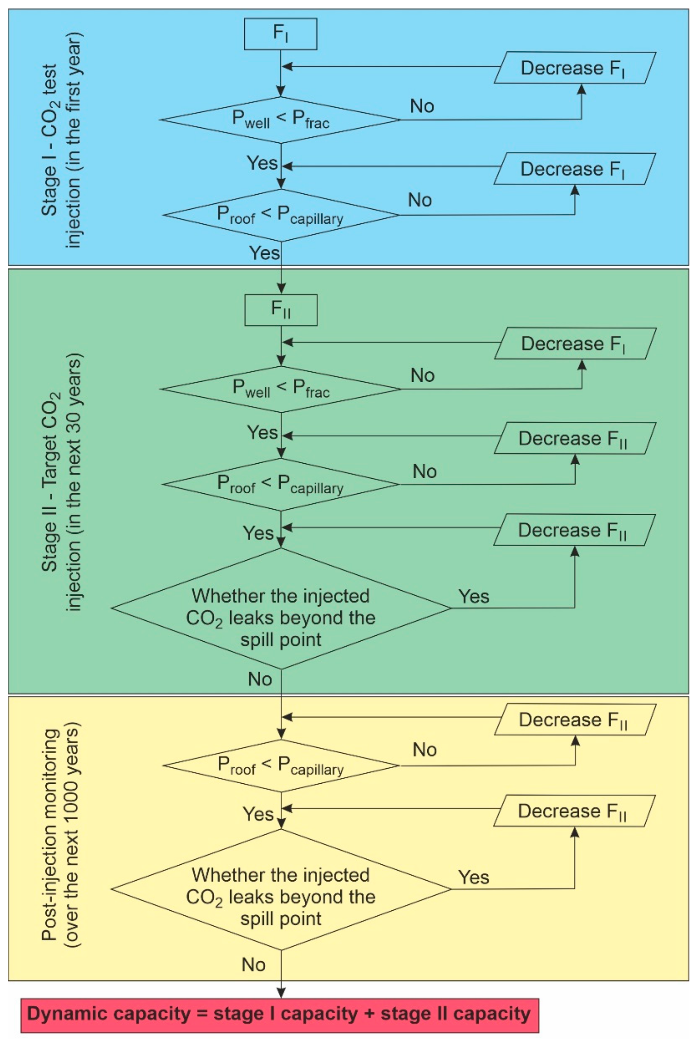
A simulation of carbon dioxide injection through a vertical well was performed for fifty different locations for each of the Konary, Sierpc, and Suliszewo structures. The distance from the designated contour (boundary) of the structure for each of the wells considered was greater than 1 km due to the potential risk of leakage of injected CO2 beyond this boundary (spill point). It was decided to inject the carbon dioxide over the entire interval of reservoir thickness. It was also decided to maximize the amount of CO2 that can be injected into the selected structure at a pressure (Pwell) that does not exceed the minimum fracturing pressure (Pfrac) calculated for each of the considered CO2 injection wells for a given structure and that does not exceed the capillary entry pressure (Pcapillary) at the roof of the structure (Proof). The diagram of this procedure is shown in Figure 5. The minimum fracturing pressures were calculated for each of the ten reservoir layers, separately for each injection well location. It was assumed that the maximum pressure increase at the top of the reservoir should not exceed the allowable value of the minimum capillary entry pressure, which is estimated to be 0.762 MPa [10,42]. Some of the fracturing pressure results obtained for the injection well located in the Konary structure with coordinates (9500; 5000) are presented in the Supplementary Materials in Table S1. The table shows the maximum pressures in each layer, assuming that the stated capillary entry pressure is not exceeded. As can be seen, the fracturing pressure was not exceeded in any of the layers, even after taking into account Peaceman’s correction [63,64] related to simulations on model cells larger than the size of the injection well. It was also required that the CO2 does not migrate the defined contour of the structure (spill point) by specifying the saturation of the rock with carbon dioxide that does not reach 10% in any cell of the model calculation grid located at the boundary of the structure.
The process of CO2 injection for each of the structures was divided into two stages: Stage I—test injection (first year) and Stage II—target injection (next 30 years) (similar to [58]), a total of 31 years. In both the first and second stages, the efficiency of the CO2 injection into the structure was assumed to be constant throughout each stage (FI—flow rate in Stage I during the first year and FII—flow rate in Stage II during the last 30 years) (see Figure 5). This division in periods of CO2 injection allowed for an increase in the amount of injected CO2 during the target injection without exceeding the permitted pressures.
In addition, for each injection well site, after an injection period of 31 years (1 year and an additional 30 years), a simulation was conducted to monitor the behavior of the injected CO2 plume and the changes in pressure after injecting carbon dioxide into the structure for over 1000 years. The monitoring was carried out to ensure that the allowable pressures in the structure were not exceeded over a given period and to ensure that the injected carbon dioxide did not leak beyond the boundary of the structure (spill point) after injection.
2.6. Determination of the CO2 Storage Efficiency
In the article, the CO2 storage efficiency for each of the three selected structures was determined by comparing the calculated total theoretical storage capacity of carbon dioxide with the dynamic CO2 storage capacity determined for each CO2 injection well site individually. The values obtained were compared with the calculated total theoretical CO2 storage capacity:
where:
Edyn—CO2 storage efficiency [%]
Mdyn—dynamic CO2 storage capacity [kg]
MT+R—total theoretical CO2 storage capacity (as a sum of the theoretical CO2 storage capacity and the capacity from dissolution in reservoir water presented in Table 5) [kg].
3. Results
The results of the calculations of theoretical CO2 storage capacity, CO2 storage capacity from dissolution in reservoir water, and total theoretical CO2 storage capacity are presented in Table 5. In addition, detailed tables regarding the data included in the calculations are shown in the Supplementary Materials for the Konary, Sierpc, and Suliszewo structures in Tables S2–S4, respectively. The estimated theoretical CO2 storage capacity for the Konary structure is 233.1 Mt CO2, for the Sierpc structure 202.55 Mt, and for the Suliszewo structure 382.59 Mt. The dissolution capacity in the Konary structure is 7.82 Mt of CO2, 2.86 Mt in the Sierpc structure, and 8.28 Mt in the Suliszewo structure. Thus, the total theoretical capacity of CO2 storage for the Konary structure is 240.91 Mt of CO2, 205.41 Mt for the Sierpc structure, and 390.87 Mt for the Suliszewo structure.
The simulation of CO2 injection into the Konary structure shows a wide range of dynamic storage capacity values (in both variant I and II) for the considered injection period of 31 years for fifty injection well locations (Table 6; presented in more detail in the Supplementary Materials in Table S5). In variant I, it is in the range of 10.86–15.52 Mt of CO2, while in variant II, lower values of average dynamic capacity were obtained, namely, between 10.19 and 14.77 Mt of CO2. The simulation of CO2 injection into the Sierpc structure showed a relatively small dynamic storage capacity, both in variant I and in variant II (Table 6, presented in more detail in the Supplementary Materials in Table S6). In variant I, the range of dynamic capacity obtained ranged from 0.21 to 1.16 Mt of CO2. However, in variant II, slightly lower values of average dynamic capacity were received, from 0.21 to 1.07 Mt of CO2. The simulation of CO2 injection into the Suliszewo structure also showed a wide range of values of dynamic storage capacity (Table 6, presented in more detail in the Supplementary Materials in Table S7), from a minimum value of 90.42 Mt of CO2 to a maximum value of 111.86 Mt of CO2.
The CO2 storage efficiency for the Konary structure was determined for two variants considered: variant I—without considering the suspected fault located near the structure, and variant II—considering the fault for all fifty locations of the CO2 injection well (Table 6, presented in more detail in the Supplementary Materials in Table S5). In variant I, the mean value of the CO2 storage efficiency was 5.48%, while the minimum and maximum values were between 4.51–6.44%, with a standard deviation of 0.39%. The values of this parameter recorded in variant II were slightly lower compared to variant I. The mean value was 5.20%, with a standard deviation of 0.38% and minimum and maximum values between 4.23–6.13%.
For the Sierpc structure, the CO2 storage efficiency was determined similarly to the Konary structure for the two variants considered: I and II, for all fifty CO2 injection well locations (Table 6, presented in more detail in Supplementary Materials in Table S6). The average CO2 storage efficiency for the Sierpc structure amounted to 0.46%, with a minimum and maximum range of 0.10–0.56% and a standard deviation of 0.11%. Variant II obtained slightly lower values of CO2 storage efficiency compared to variant I. The average value was 0.45% with a standard deviation of 0.09%; the minimum and maximum values ranged from 0.10–0.52%.
The results of the CO2 storage efficiency estimation for the Suliszewo structure are presented in the table (Table 6, explained in more detail in the Supplementary Materials in Table S7). The average value of this parameter was 26.42%; the minimum and maximum values ranged between 23.13 and 28.62% (with a standard deviation of 1.07%).
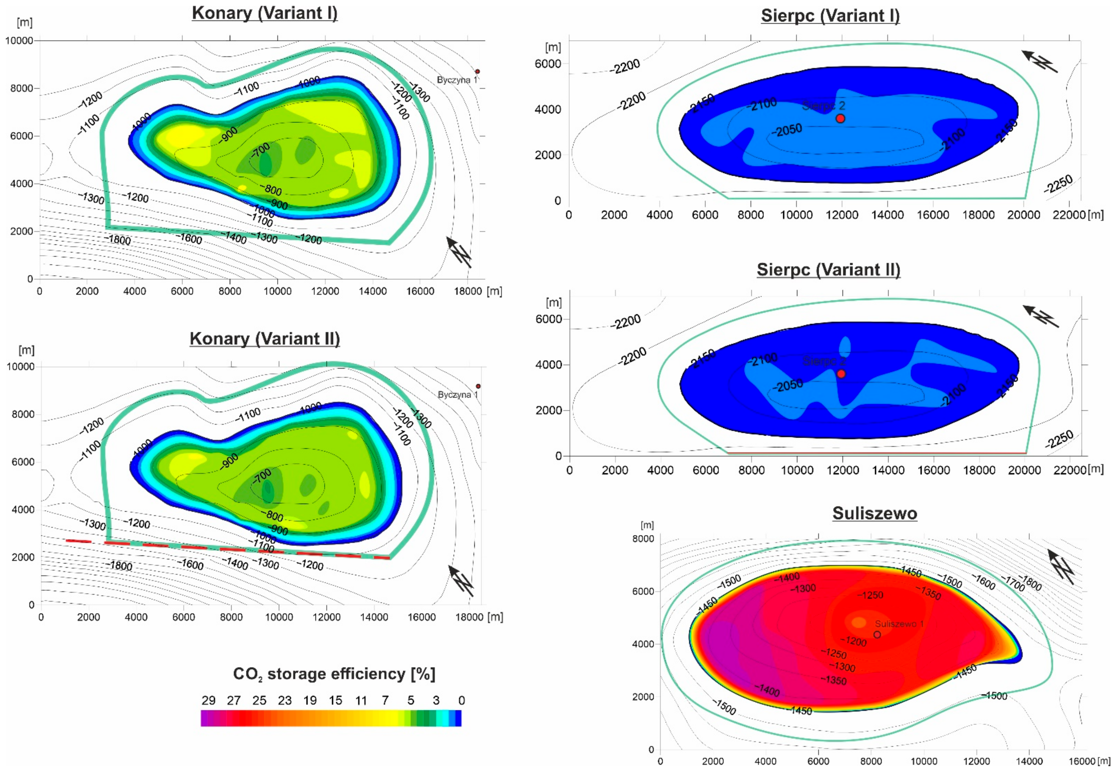
To present the obtained results of CO2 storage efficiency depending on the location of the injection well, maps of CO2 storage efficiency were prepared for each structure (Figure 6). Since fifty possible injection locations have been analyzed, they are not shown in the figure because it would make this figure ineffective. Instead, the coordinate system shown in the figure is used, and the location of the injection well is shown in the Supplementary Materials in Tables S5–S7 for each structure, respectively. Figure 6 shows what capacity can be obtained by locating one injection well at a selected site. In the Konary structure case, in variant I, the lowest values were recorded when the injection well was located at the top of the structure. An efficiency increase was observed radiating from the top of the structure to the −900 isohypse of the Komorowo formation roof and at locations below this isohypse. High efficiency was confirmed in the wells located at the structure boundary, in the area of the isohypse −800–−900 of the reservoir formation roof. On the other hand, the northern part of the structure observed the highest efficiency between the isohypses −900–−1000 of the reservoir formation roof. At this point, a maximum efficiency of 6.44% was reached (with the well in the coordinate position (6500; 6300)). After getting the highest value, it decreased in the direction of the contour delimiting the structure boundary (spill point) to reach zero at the mentioned boundary. For the II variant, similar to variant I, the lowest values were found at the top of the structure. The largest, a level of 6.13%, was recorded in a small (compared variant I) area in the N part of the structure, slightly below the isohypse −900 of the reservoir formation roof, also in the position of the well (6500; 6300). A radially propagating increase in the value of the considered parameter was observed (similar to variant I), starting from the top of the structure, while increased capacitance values were obtained only on the N and SE of the structure inclination.
In the case of the Sierpc structure, the lowest values of CO2 storage efficiency were recorded in variant I when the injection well was located near the contour of the structure. Increased efficiency values were found in the wells closest to the top of the structure, especially in the SW part. The maximum efficiency value was equal to 0.56% due to injection through the well at coordinates (14,300; 1800). A decrease in the value of efficiency was observed radially from the top to the boundary of the structure, reaching zero at the boundary. For the II variant, similar to variant I, the highest efficiency values were found near the top of the structure. The highest value, amounting to 0.52%, was recorded closer to the center of the top of the structure compared to the first variant, this time in the well at position (13,600; 3400). A radially propagating decrease in efficiency was observed towards the contour delimiting the boundary of the structure (similar to variant I), with a small area of reduced values near E from the top of the structure.
In the Suliszewo structure case, the lowest values of the CO2 storage efficiency were recorded when the injection well was located at the top of the structure. An increase in the efficiency was observed radiating from the top, mainly towards the structure contour, and its increased values were recorded in the SE and W parts of the structure. The highest values were found in the wells located at the structure’s W edge in the region of the isohypse −1350–−1400 of the reservoir formation roof, where the maximum value of the CO2 storage efficiency (28.62%) was reached as a result of injection through the well at the coordinates (1840; 4300). After getting the highest values, the efficiency values for the Suliszewo structure decrease towards the direction of the contour delimiting the boundary (spill point) of the structure and reaching the zero value at this boundary.
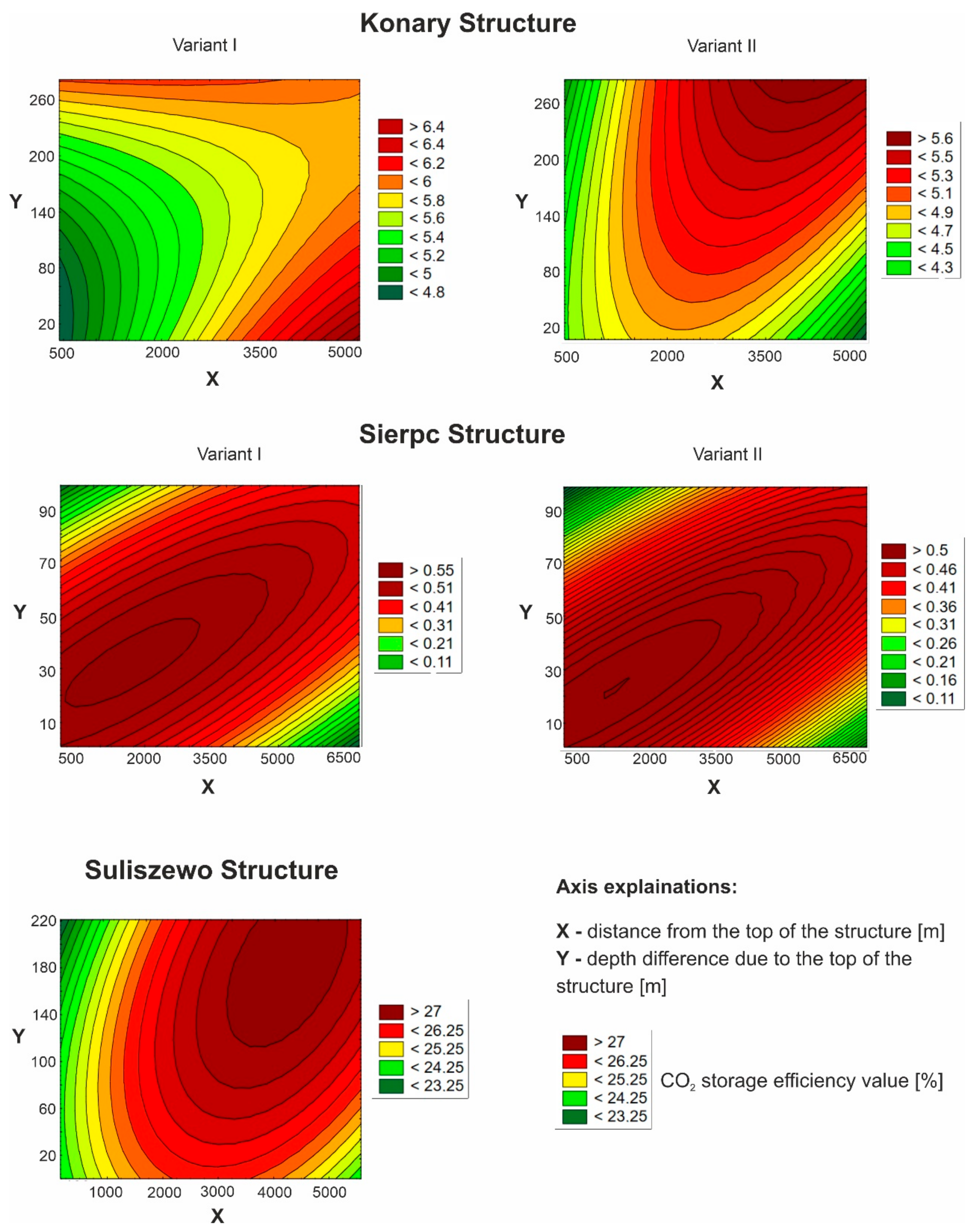
The comparison of the obtained values was also presented using color plots (Figure 7). They are used to show that storage efficiency considered structures as a function of the injection well distance from the top of the structure and the depth difference of the injection well to the top of the respective structure depth.
Figure 6 and Figure 7 show that increasing the distance of the CO2 injection well from the top of the structure leads to an increase in CO2 storage efficiency in the case of the Konary (variant I and II) and Suliszewo structures. Additional growth in the value of CO2 storage efficiency can be observed with a depth difference increase combination between the reservoir depth at the top of the structure and the injection well depth. It is most evident in the Suliszewo structure case, where this combination of the increase in the depths differences gives the highest values of CO2 storage efficiency. In the case of the Sierpc structure, the situation is just the opposite. CO2 storage efficiency decreases with an increase in the CO2 injection well distance and with increasing the difference of the depth of the reservoir in the well relative to its depth at the top of the structure.
4. Discussion
In the context of the study, it was expected that the comparison of CO2 storage efficiency for the three considered structures would give relatively similar values or ranges. However, for the studied structures, it turned out that the obtained results are different and it is not possible to define a universal value of CO2 storage efficiency. The highest values of CO2 storage efficiency, in the range of 23.13–28.62%, were obtained for the Suliszewo structure. Significantly lower values were obtained for the Konary structure, ranging from 4.23% to 6.44%. Finally, the smallest values, between 0.10 and 0.56%, were obtained for the Sierpc structure. Such a significant difference in the obtained values of CO2 storage efficiency for the three analyzed structures may result from several factors. First, the characteristics of the reservoir (mainly permeability), which affect the pressure rise during CO2 injection in the near-well zone and the upper part of the structure and thus the mobility (both vertical and horizontal) of the injected gas. Secondly, the depth of the structure, which affects the factor under consideration by changing the pressure, temperature, and mineralization of the water present in the pores of the rocks that form potential trap structures. These aspects impact the density and viscosity of both CO2 and brine, affecting the buoyancy forces and the mobility coefficient between these fluids. Cihan et al. [65] noted that lower permeability zones around the injection zone and between the faults are more extensive than the other realizations (well placements). It causes stronger pressure buildup and lowers CO2 storage capacity and thus CO2 storage efficiency. However, their work was mainly focused on reducing the pressure using brine extraction and therefore optimizing the position of the wells in this context.
The efficiencies obtained were compared with the efficiencies proposed in the CSLF method for estimating CO2 storage capacity [15]. The proportions have been held, and it was stated that structures with poor reservoir properties have a lower storage efficiency, while structures with good properties have a higher storage efficiency. But it was found that the efficiencies proposed by the CSLF method were overestimated. According to this method, the analyzed efficiency for the Sierpc structure should be about 10%, assuming that it is a poor-quality reservoir with a fault near the structure. In comparison, it was estimated to be about 0.5% according to the presented results. The Konary structure, according to the CSLF method, should have an efficiency of 20–40%, depending on whether there is a fault nearby. However, as a result of modeling, it turned out to be only 5%. The Suliszewo structure turned out to be the best structure due to good reservoir parameters and the absence of faults in its vicinity. According to the CSLF method, the efficiency should be 40%, but, as a result of the study (with the most favorable injection well location), it reached almost 29%.
When it comes to the efficiency for the two studied structures (with a fault), in the case of variant II, a slight decrease, resulting from the presence of an impermeable fault near the structure, was observed in the Konary and Sierpc structures. For the Konary structure, these values were lower by about 0.3 percentage points on average for the II variant and by about 0.01 percentage points on average for the Sierpc structure. In the Sierpc structure, there were also some locations where the CO2 storage efficiency value increased when considering the fault located near the structure (variant II). A possible reason for this slight increase is that, in both cases, the fault is found at some distance from the structure in question and the pressure increase is compensated by the propagation of the CO2 plume (and, further, the increased pressure front) in other directions.
The obtained results have shown that the CO2 injection well location within the geological structure significantly impacts the value of carbon dioxide storage efficiency. For the Suliszewo structure, where the highest values of CO2 storage efficiency (23.13–28.62%) were obtained, the difference depending on the location of the CO2 injection well is up to 5.49 percentage points. For the lower values of this efficiency obtained for the Konary structure (4.23–6.44%), the difference is 2.21 percentage points. In the case of the Sierpc structure, with the lowest efficiency values (0.10–0.56%), a difference related to the location of the injection well, amounting to 0.46 percentage points, was also observed. These differences in the values of CO2 storage efficiency associated with the location of the injection well within the structure were interpreted based on structure geometry. This aspect investigation involved analyzing the dependence of CO2 storage efficiency as a function of the injection well distance from the top of the structure and the depth difference of the reservoir in the injection well relative to the depth of the reservoir at the top of the structure (Figure 6, Figure 7). It was found that increasing the distance of the CO2 injection well from the top of the structure usually leads to an increase in CO2 storage efficiency (in the case of the Konary and Suliszewo structures). Moreover, the efficiency increases with the increasing depth difference between the well and the top of the structure. The opposite is true for the Sierpc structure—structures with poor reservoir properties where storage efficiency values decrease as the injection well move away from the top of the structure. The structure geometry combined with the other rocks properties determine the rate at which CO2 moves within the structure.
Hu et al. [36] also researched and noticed a difference in CO2 storage capacity due to the location of the injection well, although they studied storage at an oilfield. Jun et al. [37] analyzed four well patterns to define the optimal injection well pattern, placement, and operating conditions. The results showed that the optimal location and fluid rate allowed an almost eight times larger volume of CO2 to be stored compared to the base case. Okwen et al. [35] performed numerical simulations of CO2 injection to evaluate gas storage efficiency for different sedimentation environments at five other CO2 injection well locations. It allowed for finding the difference in the magnitude of this efficiency for different well locations. However, this was not the aim of the research, and only the average value of the results obtained in five locations of CO2 injection wells was compared.
What is more, Tarkowski and Uliasz-Misiak [66] presented a possible conflict of interest regarding using underground space for storage. Thus, the map shown in this article becomes a helpful tool that can solve the problem of the lack of access to some places within the range of potential CO2 storage sites.
5. Conclusions
The results of the simulation of CO2 injection performed at fifty injection well sites suggest that the dynamic capacity and CO2 storage efficiency of a given structure varies depending on the injection well site.
It was found that the efficiencies proposed by the CSLF method were overestimated. For the Suliszewo structure, the best structure in terms of both reservoir parameters and the absence of faults in its vicinity according to the CSLF method, the efficiency should be 40%, and, as a result of the study, with the most favorable location of the injection well, it reached a value of almost 29%. The Konary structure, according to the CSLF method, should have an efficiency of 20–40%, depending on whether there is a fault near it. However, as a result of modeling, it turned out to be only 5%. The efficiency for the Sierpc structure should be about 10%, assuming that it is a poor-quality reservoir with a fault near the structure, while it was estimated to be about 0.5% according to the presented results.
The comparison of CO2 storage efficiency for the considered structures of Konary, Sierpc, and Suliszewo showed that the obtained results are very different and that a universal value or range of values cannot be identified. However, several trends are worth noting: for structures with good petrophysical reservoir properties (Konary and Suliszewo), the dynamic CO2 storage capacity increases with the increase of the injection well distance from the top of the structure and with the increasing difference between the depth of the well and the top of the structure. On the other hand, the opposite occurs for a structure with poor reservoir properties (Sierpc). Notwithstanding, as the quality of the reservoir parameters porosity and permeability increases, the location of the injection well within the structure becomes more important for assessing CO2 storage efficiency.
The values of dynamic CO2 storage capacity and storage efficiency obtained by injecting the gas at the injection well site, interpreted with the maps of CO2 storage efficiency, represent an interesting tool since they allow us to determine the best location for the carbon dioxide injection well in terms of the storage capacity of this gas.
It would be advisable to analyze a more significant number of structures with a broader range of reservoir parameters and reservoir conditions to determine their influence on CO2 storage efficiency.
Supplementary Materials
The following are available online at www.mdpi.com/article/10.3390/en14248604/s1: Table S1. Maximum pressures, Peaceman correlation, and fracturing pressures in each distributed layer for the example injection well located in the Konary structure with coordinates (9500; 5000); Table S2. Estimation results of the theoretical CO2 storage capacity for the Konary structure in separate ten layers of the reservoir; Table S3. Estimation results of the theoretical CO2 storage capacity for the Sierpc structure in separate ten layers of the reservoir; Table S4. Estimation results of the theoretical CO2 storage capacity for the Suliszewo structure in separate ten layers of the reservoir; Table S5. Dynamic capacity and CO2 storage efficiency at each CO2 injection well location in the Konary structure (coordinates X and Y in relation to Figure 2); Table S6. Dynamic capacity and CO2 storage efficiency at each CO2 injection well location in the Sierpc structure (coordinates X and Y in relation to Figure 3); Table S7. Dynamic capacity and CO2 storage efficiency at each CO2 injection well location in the Suliszewo structure (coordinates X and Y in relation to Figure 4); Appendix S1.
Funding
This work was supported by the Mineral and Energy Economy Research Institute of the Polish Academy of Sciences (research subvention).
Institutional Review Board Statement
Not applicable.
Informed Consent Statement
Not applicable.
Acknowledgments
The author would like to thank Radosław Tarkowski for sharing his experience in the field of CO2 storage.
Conflicts of Interest
The author declare no conflict of interest.
References
- Goodman, A.; Bromhal, G.; Strazisar, B.; Rodosta, T.; Guthrie, W.F.; Allen, D.; Guthrie, G. Comparison of methods for geologic storage of carbon dioxide in saline formations. Int. J. Greenh. Gas Control 2013, 18, 329–342. [Google Scholar] [CrossRef]
- Tarkowski, R.; Marek, S.; Uliasz-Misiak, B. Wstępna geologiczna analiza struktur do składowania CO2 w rejonie Bełchatowa (Preliminary geological analysis of structures to store CO2 within the Bełchatów area). Gospod. Surowcami Miner. Miner. Resour. Manag. 2009, 25, 37–45. [Google Scholar]
- Popova, O.H.; Small, M.J.; McCoy, S.T.; Thomas, A.C.; Karimi, B.; Goodman, A.; Carter, K.M. Comparative analysis of carbon dioxide storage resource assessment methodologies. Environ. Geosci. 2012, 19, 105–124. [Google Scholar] [CrossRef]
- U.S. Department of Energy; Office of Fossil Energy National Energy Technology Laboratory. The United States Carbon Utilization and Storage Atlas, 4th ed.; NETL: Pittsburgh, PA, USA, 2012. [Google Scholar]
- Gorecki, C.; Sorensen, J.; Bremer, J.; Knudsen, D.J.; Smith, S.A.; Steadman, E.N.; Harju, J.A. Development of Storage Coefficients for Carbon Dioxide Storage in Deep Saline Formations; Technical Study Report No. 2009/13; Global CCS Institute: Melbourne, Australia, 2009; pp. 1–118. [Google Scholar]
- Goodman, A.; Hakala, A.; Bromhal, G.; Deel, D.; Rodosta, T.; Frailey, S.; Small, M.; Allen, D.; Romanov, V.; Fazio, J.; et al. U.S. DOE methodology for the development of geologic storage potential for carbon dioxide at the national and regional scale. Int. J. Greenh. Gas Control 2011, 5, 952–965. [Google Scholar] [CrossRef]
- Bachu, S.; Bonijoly, D.; Bradshaw, J.; Burruss, R.; Holloway, S.; Christensen, N.P.; Mathiassen, O.M. CO2 storage capacity estimation: Methodology and gaps. Int. J. Greenh. Gas Control 2007, 1, 430–443. [Google Scholar] [CrossRef] [Green Version]
- Carbon Sequestration Leadership Forum. Comparison between Methodologies Recommended for Estimation of CO2 Storage Capacity in Geological Media by the CSLF Task Force on CO2 Storage Capacity Estimation and the USDOE Capacity and Fairways Subgroup of the Regional Carbon Sequestration Partnership; Report No CSLF-T-2008- 04. 2008, pp. 1–17. Available online: https://citeseerx.ist.psu.edu/viewdoc/download?doi=10.1.1.352.9809&rep=rep1&type=pdf (accessed on 14 August 2021).
- Bachu, S. Review of CO2 storage efficiency in deep saline aquifers. Int. J. Greenh. Gas Control 2015, 40, 188–202. [Google Scholar] [CrossRef]
- Espinoza, D.N.; Santamarina, J.C. CO2 breakthrough—Caprock sealing efficiency and integrity for carbon geological storage. Int. J. Greenh. Gas Control 2017, 66, 218–229. [Google Scholar] [CrossRef] [Green Version]
- Gorecki, C.D.; Ayash, S.C.; Liu, G.; Braunberger, J.R.; Dotzenrod, N.W. A comparison of volumetric and dynamic CO2 storage resource and efficiency in deep saline formations. Int. J. Greenh. Gas Control 2015, 42, 213–225. [Google Scholar] [CrossRef]
- Bradshaw, J.; Allinson, G.; Bradshaw, B.E.; Nguyen, V.; Rigg, A.J.; Spencer, L.; Wilson, P. Australia’s CO2 geological storage potential and matching of emission sources to potential sinks. Energy 2004, 29, 1623–1631. [Google Scholar] [CrossRef]
- Van der Meer, L.G.H. The CO2 storage efficiency of aquifers. Energy Convers. Manag. 1995, 36, 513–518. [Google Scholar] [CrossRef]
- Uliasz-Misiak, B. Pojemność Podziemnego Składowania CO2 dla Wybranych Mezozoicznych Poziomów Wodonośnych Oraz Złóż Węglowodorów w Polsce; Studia Rozprawy Monografie 142; IGSMiE PAN: Kraków, Poland, 2008; ISBN 9788360195062. [Google Scholar]
- Geoological Survey of Denmark and Greenland EU GeoCapacity Assessing European Capacity for Geological Storage of Carbon Dioxide. Project no SES6-518318. D26, WP 4 Report, Capacity Standards and Site Selection Criteria. 2006, pp. 1–45. Available online: https://www.globalccsinstitute.com/archive/hub/publications/162178/assessing-european-capacity-geological-storage-carbon-dioxide.pdf (accessed on 14 August 2021).
- Chadwick, A.; Arts, R.; Bernstone, C.; May, F.; Thibeau, S.; Zweigel, P. Best practice for the storage of CO2 in saline aquifers. In Observations and Guidelines from the SACS and CO2STORE Projects; British Geological Survey Occasional Publication 14: Nottingham, UK, 2006; ISBN 9780852726105. [Google Scholar]
- Uliasz-Misiak, B. Klasyfikacje pojemności i kryteria wyboru miejsc składowania CO2. Gospod. Surowcami Miner. Miner. Resour. Manag. 2009, 25, 97–108. [Google Scholar]
- Określenie (aktualizacja) bilansu sekwestracyjnego dla Polski [in:] Rozpoznanie formacji i struktur do bezpiecznego geo-logicznego składowania CO2 wraz z ich programem monitorowania (Assessment of formations and structures suitable for safe CO2 geological storage (in Poland) including the monitoring plans). Report—Segment I. 2013; pp. 1–175. Available online: https://skladowanie.pgi.gov.pl/twiki/pub/CO2/WynikiPrac/I-2.pdf (accessed on 13 August 2021).
- Vangkilde-Pedersen, T.; Anthonsen, K.L.; Smith, N.; Kirk, K.; Neele, F.; van der Meer, B.; Le Gallo, Y.; Bossie-Codreanu, D.; Wojcicki, A.; Le Nindre, Y.M.; et al. Assessing European capacity for geological storage of carbon dioxide—the EU GeoCapacity project. Energy Procedia 2009, 1, 2663–2670. [Google Scholar] [CrossRef] [Green Version]
- Carbon Sequestration Leadership Forum. 2021 Carbon Sequestration Technology Roadmap. 2021, pp. 1–69. Available online: https://www.cslforum.org/cslf/sites/default/files/CSLF_Tech_Roadmap_2021_final_0.pdf (accessed on 14 September 2021).
- Van der Meer, L.G.H.; Egberts, P.J.P.P. A General Method for Calculating Subsurface CO2 Storage Capacity. In Proceedings of the Offshore Technology Conference, OTC 08-“Waves of Change”, Houston, TX, USA, 5–8 May 2008; Volume 2. [Google Scholar]
- Van der Meer, L.G.H.; Yavuz, F. CO2 storage capacity calculations for the Dutch subsurface. Energy Procedia 2009, 1, 2615–2622. [Google Scholar] [CrossRef] [Green Version]
- Tarkowski, R. CO2 storage capacity of geological structures located within Polish Lowlands’ Mesozoic formations. Gospod. Surowcami Miner. Miner. Resour. Manag. 2008, 24, 101–112. [Google Scholar]
- Willscher, B.; May, F.; Tarkowski, R.; Uliasz-Misiak, B.; Wójcicki, A. EU GeoCapacity—Towards a Europe-wide GIS of CO2 Emittants and Storage Sites. Zeitschrift Geol. Wissenschaften 2008, 36, 303–320. [Google Scholar]
- Tarkowski, R.; Uliasz-Misiak, B.; Wójcicki, A. CO2 storage capacity of deep aquifers and hydrocarbon fields in Poland—EU GeoCapacity Project results. Energy Procedia 2009, 1, 2671–2677. [Google Scholar] [CrossRef] [Green Version]
- Šliaupa, S.; Lojka, R.; Tasáryova, Z.; Kolejka, V.; Hladík, V.; Kotulová, J.; Kucharič, L.; Fejdi, V.; Wójcicki, A.; Tarkowski, R.; et al. CO2 storage potential of sedimentary basins of Slovakia, the Czech Republic, Poland and the Baltic States. Geol. Q. 2013, 57, 219–232. [Google Scholar] [CrossRef] [Green Version]
- Marek, S.; Dziewińska, L.; Tarkowski, R. The possibilities of underground CO2 storage in the Zaosie Anticline Introduction. Gospod. Surowcami Miner. Miner. Resour. Manag. 2011, 27, 89–107. [Google Scholar]
- Tarkowski, R.; Dziewińska, L.; Marek, S. The Characteristics of Selected Potential Geological Structures for CO2 Underground Storage in Mezozoic Deposits of the Sczecin-Mogilno-Uniejów Trough; Wydawnictwo IGSMiE PAN: Kraków, Poland, 2014; ISBN 9788362922307. [Google Scholar]
- Luboń, K. The effect of providing details to the model of a geological structure on the assessment of CO₂ storage capacity. Geol. Geophys. Environ. 2016, 42, 449–458. [Google Scholar] [CrossRef] [Green Version]
- Luboń, K. CO2 storage capacity of a deep aquifer depending on the injection well location and cap rock capillary pressure. Gospod. Surowcami Miner. Miner. Resour. Manag. 2020, 36, 173–196. [Google Scholar] [CrossRef]
- Labus, K.; Tarkowski, R.; Wdowin, M. Assessment of CO2 Sequestration capacity based on hydrogeochemical model of water-rock-gas interactions in the potential storage site within the BeŁchatów area (Poland). Gospod. Surowcami Miner. Miner. Resour. Manag. 2010, 26, 69–84. [Google Scholar]
- Labus, K.; Tarkowski, R.; Wdowin, M. Modeling gas–rock–water interactions in carbon dioxide storage capacity assessment: A case study of Jurassic sandstones in Poland. Int. J. Environ. Sci. Technol. 2015, 12, 2493–2502. [Google Scholar] [CrossRef] [Green Version]
- Stopa, J.; Janiga, D.; Wojnarowski, P.; Czarnota, R. Optimization of well placement and control to maximize CO2 trapping during geologic sequestration. AGH Drill. Oil Gas 2016, 33, 93–104. [Google Scholar] [CrossRef] [Green Version]
- Hajiabadi, S.H.; Bedrikovetsky, P.; Borazjani, S.; Mahani, H. Well Injectivity during CO2 Geosequestration: A Review of Hydro-Physical, Chemical, and Geomechanical Effects. Energy Fuels 2021, 35, 9240–9267. [Google Scholar] [CrossRef]
- Okwen, R.; Yang, F.; Frailey, S. Effect of geologic depositional environment on CO2 storage efficiency. Energy Procedia 2014, 63, 5247–5257. [Google Scholar] [CrossRef] [Green Version]
- Hu, T.; Xu, T.-F.; Tian, H.-L.; Zhou, B.; Yang, Y.-Z. A study of CO2 injection well selection in the naturally fractured undulating formation in the Jurong Oilfield, China. Int. J. Greenh. Gas Control 2021, 109, 103377. [Google Scholar] [CrossRef]
- Jun, C.; Kim, M.; Shin, H. Optimization of well placement and operating conditions for various well patterns in CO2 sequestration in the Pohang Basin, Korea. Int. J. Greenh. Gas Control 2019, 90, 102810. [Google Scholar] [CrossRef]
- Urych, T.; Smoliński, A. Numerical Modeling of CO2 Migration in Saline Aquifers of Selected Areas in the Upper Silesian Coal Basin in Poland. Energies 2019, 12, 3093. [Google Scholar] [CrossRef] [Green Version]
- White, D.J. 3D architecture of the Aquistore reservoir: Implications for CO2 flow and storage capacity. Int. J. Greenh. Gas Control 2018, 71, 74–85. [Google Scholar] [CrossRef]
- Uliasz-Misiak, B.; Tarkowski, R. Ranking struktur do podziemnego składowania CO2 zlokalizowanych na Niżu Polskim. In Potencjalne Struktury Geologiczne do Składowania CO2 w utworach Niżu Polskiego (Charakterystyka oraz Ranking). Studia, Rozprawy, Monografie, 164; Tarkowski, R., Ed.; Wydawnictwo IGSMiE PAN: Kraków, Poland, 2010; pp. 112–123. [Google Scholar]
- Marek, S.; Tarkowski, R.; Dziewińska, L. Potencjalne struktury geologiczne do składowania CO2. In Potencjalne Struktury Geologiczne do Składowania CO2 w Utworach Niżu Polskiego (Charakterystyka oraz Ranking). Studia, Rozprawy, Monografie, 164; Tarkowski, R., Ed.; Wydawnictwo IGSMiE PAN: Kraków, Poland, 2010; pp. 16–111. [Google Scholar]
- Luboń, K. Ocena efektywności geologicznego składowania CO2 w poziomach wodonośnych jury dolnej Niżu Polskiego. In Studia, Rozprawy, Monografie 211; Wydawnictwo IGSMiE PAN: Kraków, Poland, 2020; ISBN 9788395638053. [Google Scholar]
- Luboń, K.; Tarkowski, R. Numerical simulation of hydrogen injection and withdrawal to and from a deep aquifer in NW Poland. Int. J. Hydrog. Energy 2020, 45, 2068–2083. [Google Scholar] [CrossRef]
- Luboń, K.; Tarkowski, R. Influence of capillary threshold pressure and injection well location on the dynamic CO2 and H2 storage capacity for the deep geological structure. Int. J. Hydrog. Energy 2021, in press. [Google Scholar] [CrossRef]
- Marek, S.; Cichy, H. Dokumentacja wynikowa otworu Konary IG-1; Państwowy Instytut Geologiczny: Warszawa, Poland, 1974. [Google Scholar]
- Tarkowski, R. (Mineral and Energy Economy Research Institute of the Polish Academy of Sciences, Krakow, Poland); Marek, S. (Polish Geological Institute, Warszawa, Poland); Dziewińska, L. (Polish Geological Institute, Warszawa, Poland). Struktury Geologiczne Mezozoiku Niżu Polskiego do Podziemnego Składowania CO2 –część IV. Praca Statutowa, Opracowanie Archiwalne IGSMiE PAN. (Unpublished work). 2011; 1–31. [Google Scholar]
- Atlas Hydrochemiczny i Hydrodynamiczny Paleozoiku i Mezozoiku Oraz Ascenzyjnego Zasolenia wód Podziemnych na Niżu Polskim–1:1 000 000; Bojarski, L. (Ed.) Państwowy Instytut Geologiczny: Warszawa, Poland, 1996. [Google Scholar]
- Górecki, W.; Hajto, M.; Strzetelski, W.; Szczepański, A. Dolnokredowy oraz dolnojurajski zbiornik wód geotermalnych na Niżu Polskim. Przegląd Geol. 2010, 58, 589–593. [Google Scholar]
- Ryll, A. Stratygrafia i paleogeografia. Jura środkowa. W: Budowa geologiczna niecki warszawskiej (płockiej) i jej podłoża. Pr. Inst. Geol. 1983, 103, 138–148. [Google Scholar]
- Pieńkowski, G. The epicontinental Lower Jurassic of Poland. Pol. Geol. Inst. Spec. Pap. 2004, 12, 5–154. [Google Scholar]
- Feldman-Olszewska, A.; Adamczak-Biały, T.; Begier, A. Charakterystyka poziomów zbiornikowych i uszczelniających formacji jury i triasu północnego Mazowsza pod kątem geologicznego składowania CO2 na podstawie danych z głębokich otworów wiertniczych. Biul. Państwowego Inst. Geol. 2012, 448, 27–46. [Google Scholar]
- Marek, S.; Dziewińska, L.; Tarkowski, R. Możliwości wykorzystania antyklin Choszczna i Suliszewa do podziemnego składowania CO2. Przegląd Górniczy 2013, 11, 76–89. [Google Scholar]
- Tarkowski, R. (Mineral and Energy Economy Research Institute of the Polish Academy of Sciences, Krakow, Poland); Marek, S. (Polish Geological Institute, Warszawa, Poland); Dziewińska, L. (Polish Geological Institute, Warszawa, Poland). Struktury geologiczne Mezozoiku Niżu Polskiego do Podziemnego Składowania CO2—część V. Praca Statutowa, Opracowanie Archiwalne IGSMiE PAN. (Unpublished work). 2012; 1–55. [Google Scholar]
- Pruess, K. ECO2N: A TOUGH2 Fluid Property Module for Mixtures of Water, NaCl, and CO2; Earth Sciences Division, Lawrence Berkeley National Laboratory: Berkely, CA, USA, 2005; pp. 1–66. [Google Scholar]
- Pruess, K.; Oldenburg, C.; Moridis, G. TOUGH2 User’s Guide. Report LBNL-43134; Lawrence Berkeley National Laboratory: Berkeley, CA, USA, 1999; p. 210. [Google Scholar]
- Doughty, C.; Pruess, K. Modeling Supercritical Carbon Dioxide Injection in Heterogeneous Porous Media. Vadose Zone J. 2004, 3, 837–847. [Google Scholar] [CrossRef]
- Lothe, A.E.; Emmel, B.; Grøver, A.; Bergmo, P.E. CO2 storage modelling and capacity estimation for the Trøndelag Platform, offshore Norway—using a basin modelling approach. Energy Procedia 2014, 63, 3648–3657. [Google Scholar] [CrossRef] [Green Version]
- Modelowania Dynamiczne Procesów Zatłaczania CO2 do Składowiska [in:] Rozpoznanie Formacji i Struktur do Bezpiec-znego Geologicznego Składowania CO2 Wraz z ich Programem Monitorowania (Assessment of Formations and Structures Suitable for safe CO2 Geological Storage (in Poland) Including the Monitoring Plans). Report—Segment II. 2013; pp. 1–426. Available online: https://skladowanie.pgi.gov.pl/twiki/pub/CO2/WynikiBelchatowSegII/Be%b3chat%f3w_II.pdf (accessed on 13 August 2021).
- TOUGHREACT Example: CO2 Disposal in Deep Saline Aquifers. PetraSim 2016.1. Thunderhead Eng. 2016, pp. 1–24. Available online: https://www.thunderheadeng.com/wp-content/uploads/dlm_uploads/2016/01/examples_toughreact_CO2_Disposal.pdf (accessed on 8 August 2016).
- Zhao, H. CO2 Calculator. A Web Computational Tool. Available online: http://www.energy.psu.edu/tools/CO2-EOS/ (accessed on 19 July 2017).
- Span, R.; Wagner, W. A new equation of state for carbon dioxide covering the fluid region from the triple-point temperature to 1100 K at pressures up to 800 MPa. J. Phys. Chem. Ref. Data 1996, 25, 1509–1596. [Google Scholar] [CrossRef] [Green Version]
- Bachu, S.; Adams, J.J. Sequestration of CO2 in geological media in response to climate change: Capacity of deep saline aquifers to sequester CO2 in solution. Energy Convers. Manag. 2003, 44, 3151–3175. [Google Scholar] [CrossRef]
- Peaceman, D.W. Interpretation of well-block pressures in numerical reservoir simulation. Soc. Pet. Eng. J. 1978, 6893, 183–194. [Google Scholar] [CrossRef]
- Peaceman, D.W. Interpretation of Well-Block Pressures in Numerical Reservoir Simulation with Nonsquare Grid Blocks and Anisotropic Permeability. Soc. Pet. Eng. J. 1983, 23, 531–543. [Google Scholar] [CrossRef]
- Cihan, A.; Birkholzer, J.T.; Bianchi, M. Optimal well placement and brine extraction for pressure management during CO2 sequestration. Int. J. Greenh. Gas Control 2015, 42, 175–187. [Google Scholar] [CrossRef] [Green Version]
- Tarkowski, R.; Uliasz-Misiak, B. Use of underground space for the storage of selected gases (CH4, H2, and CO2)–possible conflicts of interest. Gospod. Surowcami Miner. Miner. Resour. Manag. 2021, 37, 141–160. [Google Scholar] [CrossRef]
Figure 1.
Location of the structures: Konary, Sierpc, and Suliszewo in Poland and Europe against the background of the Lower Jurassic rocks.
Figure 1.
Location of the structures: Konary, Sierpc, and Suliszewo in Poland and Europe against the background of the Lower Jurassic rocks.

Figure 2.
The area selected for modeling against the background of the Konary structural map and the AB cross-sections of the reservoir, illustrating permeability and porosity changes (based on [46] with the author’s additions).
Figure 2.
The area selected for modeling against the background of the Konary structural map and the AB cross-sections of the reservoir, illustrating permeability and porosity changes (based on [46] with the author’s additions).

Figure 3.
The area selected for modeling against the background of the Sierpc structural map and the AB cross-sections of the reservoir, illustrating permeability and porosity changes (based on [53] with the author’s additions).
Figure 3.
The area selected for modeling against the background of the Sierpc structural map and the AB cross-sections of the reservoir, illustrating permeability and porosity changes (based on [53] with the author’s additions).

Figure 4.
The area selected for modeling against the background of the Suliszewo structural map and the AB cross-sections of the reservoir, illustrating permeability and porosity changes (based on [52] with the author’s additions).
Figure 4.
The area selected for modeling against the background of the Suliszewo structural map and the AB cross-sections of the reservoir, illustrating permeability and porosity changes (based on [52] with the author’s additions).

Figure 5.
Procedure for determining the dynamic CO2 storage capacity for selected structures; FI—CO2 flow rate during Stage I—test injection; FII—CO2 flow rate during Stage II—target injection; Pwell—bottom well pressure; Pfrac—minimum fracturing pressure; Pcapillary—cap rock capillary entry pressure; Proof—pressure at the top of the structure.

Figure 6.
Maps of the CO2 storage efficiency in the Konary, Sierpc, and Suliszewo structures as a function of injection well location.
Figure 6.
Maps of the CO2 storage efficiency in the Konary, Sierpc, and Suliszewo structures as a function of injection well location.

Figure 7.
2D X–Y color plots of CO2 storage efficiency against the distance from the top of the structure and the depth difference between the top of the Konary, Sierpc, and Suliszewo structures.
Figure 7.
2D X–Y color plots of CO2 storage efficiency against the distance from the top of the structure and the depth difference between the top of the Konary, Sierpc, and Suliszewo structures.


Table 1.
Summary of the data assumed for CO2 injection modeling for Konary, Sierpc, and Suliszewo structures (own work based on [41,45,46,47,48,52,53]).
| Geological Data | Konary Structure | Sierpc Structure | Suliszewo Structure |
|---|---|---|---|
| Area of the structure | 47.39 km2 | 59.76 km2 | 51.61 km2 |
| Isohypse represents the boundary of the structure (spill point) | −1000 m | −2150 m | −1450 m |
| Thickness of the reservoir in the wells within the structure | Byczyna 1–94 m | Sierpc 2: 46 m | Suliszewo 1: 89 m |
| Depth of the reservoir in the well within the structure | Byczyna 1: 1832–1926 m | Sierpc 2: 2190.0–2236 m | Suliszewo 1: 1293–1382 m |
| Density of the reservoir rocks | 2542 kg/m3 | 2500 kg/m3 | 2390 kg/m3 |
| Geothermal gradient (reservoir temperature) | 2.9 °C/100 m (35.8–48 °C) | 2.1 °C/100 m (58.6–61.2 °C) | 3.5 °C/100 m (63.0–65.1 °C) |
| Pressure gradient(reservoir pressure) | 1040 hPa/10 m (9.12–9.94 MPa) | 1000 hPa/10 m (20.41–22.03 MPa) | 975 hPa/10 m (13.20–13.78 MPa) |
| Brine salinity | 42 kg/m3 | 150 kg/m3 | 100 kg/m3 |
| Stratigraphic unit of the reservoir | Upper Pliensbachian (Domerian): Komorowo Formation | Upper Pliensbachian (Domerian): Komorowo=Drzewice Formation | Upper Pliensbachian (Domerian): Komorowo Formation |
| Lithology of the reservoir | Sandstones (~80%) with claystones and mudstones interbeds | Sandstones (~80–85%) with claystones and mudstones interbeds | Sandstones (90%) with claystones and mudstones interbeds |
| Stratigraphic unit of seal | Lower Toarcian (Ciechocinek Formation) | Lower Toarcian (Ciechocinek Formation) | Lower Toarcian (Ciechocinek = Gryfice Formation) |
| Lithology of the seal | claystones and mudstones with sandstone interbeds, total thickness 125 m | claystones and mudstones with sandstone interbeds, total thickness 77.5 m | claystones and mudstones with sandstone interbeds, total thickness 67.5 m |
Table 2.
Characteristics of the ten separate reservoir layers within the Komorowo Lower Jurassic Formation of the Konary structure in the Byczyna 1 well.
Table 2.
Characteristics of the ten separate reservoir layers within the Komorowo Lower Jurassic Formation of the Konary structure in the Byczyna 1 well.
| No | Depth Interval [m] | Thickness [m] | Average Permeability [mD] | Average Porosity [decimal] |
|---|---|---|---|---|
| 1 | 1832–1860 | 28 | 900.00 | 0.1675 |
| 2 | 1860–1865 | 5 | 330.00 | 0.16 |
| 3 | 1865–1881 | 16 | 725.00 | 0.1663 |
| 4 | 1881–1888 | 7 | 63.57 | 0.0986 |
| 5 | 1888–1891 | 3 | 101.67 | 0.1033 |
| 6 | 1891–1915 | 24 | 435.42 | 0.1408 |
| 7 | 1915–1917 | 2 | 90.00 | 0.095 |
| 8 | 1917–1919 | 2 | 300.00 | 0.1 |
| 9 | 1919–1922 | 3 | 10.00 | 0.03 |
| 10 | 1922–1926 | 4 | 195.00 | 0.095 |
Table 3.
Characteristics of the ten separate reservoir layers within the Drzewice (= Komorowo) Lower Jurassic Formation of the Sierpc structure in the Sierpc 2 well.
Table 3.
Characteristics of the ten separate reservoir layers within the Drzewice (= Komorowo) Lower Jurassic Formation of the Sierpc structure in the Sierpc 2 well.
| No | Depth Interval [m] | Thickness [m] | Average Permeability [mD] | Average Porosity [decimal] |
|---|---|---|---|---|
| 1 | 2190–2193 | 3.0 | 47.93 | 0.1527 |
| 2 | 2193–2194.5 | 1.5 | 10.03 | 0.1271 |
| 3 | 2194.5–2198.5 | 4.0 | 55.82 | 0.1513 |
| 4 | 2198.5–2200 | 1.5 | 10.64 | 0.1283 |
| 5 | 2200–2203.5 | 3.5 | 20.53 | 0.1366 |
| 6 | 2203.5–2205.5 | 2.0 | 2.38 | 0.1046 |
| 7 | 2205.5–2212 | 6.5 | 27.64 | 0.1379 |
| 8 | 2212–2215.5 | 3.5 | 89.51 | 0.1591 |
| 9 | 2215.5–2226 | 10.5 | 19.43 | 0.1326 |
| 10 | 2226–2236 | 10.0 | 65.97 | 0.1565 |
Table 4.
Characteristics of the ten separate reservoir layers within the Komorowo Lower Jurassic Formation of the Suliszewo structure in the Suliszewo 1 well.
Table 4.
Characteristics of the ten separate reservoir layers within the Komorowo Lower Jurassic Formation of the Suliszewo structure in the Suliszewo 1 well.
| No | Depth Interval [m] | Thickness [m] | Average Permeability [mD] | Average Porosity [decimal] |
|---|---|---|---|---|
| 1 | 1293–1314.5 | 21.5 | 2415.92 | 0.258 |
| 2 | 1314.5–1322.25 | 7.75 | 2692.04 | 0.2613 |
| 3 | 1322.25–1326.25 | 4 | 1081.47 | 0.2166 |
| 4 | 1326.25–1337.5 | 11.25 | 3669.65 | 0.278 |
| 5 | 1337.5–1344.75 | 7.25 | 1714.50 | 0.2429 |
| 6 | 1344.75–1355.75 | 11 | 3183.63 | 0.2632 |
| 7 | 1355.75–1362.25 | 6.5 | 21.44 | 0.0763 |
| 8 | 1362.25–1368 | 5.75 | 1535.20 | 0.2277 |
| 9 | 1368–1372.25 | 4.25 | 8.77 | 0.0524 |
| 10 | 1372.25–1382 | 9.75 | 1176.01 | 0.2227 |
Table 5.
Summary of the theoretical capacity, capacity from dissolution in reservoir water, and total theoretical capacity for the Konary, Sierpc, and Suliszewo structures.
Table 5.
Summary of the theoretical capacity, capacity from dissolution in reservoir water, and total theoretical capacity for the Konary, Sierpc, and Suliszewo structures.
| CO2 Storage Capacity [Mt CO2] | Konary | Sierpc | Suliszewo |
|---|---|---|---|
| Theoretical MT | 233.10 | 202.55 | 382.59 |
| From dissolution in reservoir water | 7.82 | 2.86 | 8.28 |
| Total theoretical MT+R | 240.91 | 205.41 | 390.87 |
Table 6.
Summary of the dynamic storage capacity and storage efficiency of CO2 in selected structures.
Table 6.
Summary of the dynamic storage capacity and storage efficiency of CO2 in selected structures.
| Konary | Sierpc | Suliszewo | ||||
|---|---|---|---|---|---|---|
| Variant I | Variant II | Variant I | Variant II | |||
| Dynamic capacity Mdyn [Mt CO2] | Minimum | 10.86 | 10.19 | 0.21 | 0.21 | 90.42 |
| Maximum | 15.52 | 14.77 | 1.16 | 1.07 | 111.86 | |
| Average | 13.21 | 12.53 | 0.94 | 0.92 | 103.28 | |
| Standard deviation | 0.95 | 0.91 | 0.23 | 0.19 | 4.20 | |
| CO2 storage efficiency Edyn [%] | Minimum | 4.51 | 4.23 | 0.10 | 0.10 | 23.13 |
| Maximum | 6.44 | 6.13 | 0.56 | 0.52 | 28.62 | |
| Average | 5.48 | 5.20 | 0.46 | 0.45 | 26.42 | |
| Standard deviation | 0.39 | 0.38 | 0.11 | 0.09 | 1.07 | |
Publisher’s Note: MDPI stays neutral with regard to jurisdictional claims in published maps and institutional affiliations. |
© 2021 by the author. Licensee MDPI, Basel, Switzerland. This article is an open access article distributed under the terms and conditions of the Creative Commons Attribution (CC BY) license (https://creativecommons.org/licenses/by/4.0/).
Share and Cite
MDPI and ACS Style
Luboń, K. Influence of Injection Well Location on CO2 Geological Storage Efficiency. Energies 2021, 14, 8604. https://doi.org/10.3390/en14248604
AMA Style
Luboń K. Influence of Injection Well Location on CO2 Geological Storage Efficiency. Energies. 2021; 14(24):8604. https://doi.org/10.3390/en14248604
Chicago/Turabian StyleLuboń, Katarzyna. 2021. "Influence of Injection Well Location on CO2 Geological Storage Efficiency" Energies 14, no. 24: 8604. https://doi.org/10.3390/en14248604
Note that from the first issue of 2016, this journal uses article numbers instead of page numbers. See further details here.