Trip Based Modeling of Fuel Consumption in Modern Heavy-Duty Vehicles Using Artificial Intelligence

Abstract

Heavy-duty trucks contribute approximately 20% of fuel consumption in the United States of America (USA). The fuel economy of heavy-duty vehicles (HDV) is affected by several real-world parameters like road parameters, driver behavior, weather conditions, and vehicle parameters, etc. Although modern vehicles comply with emissions regulations, potential malfunction of the engine, regular wear and tear, or other factors could affect vehicle performance. Predicting fuel consumption per trip based on dynamic on-road data can help the automotive industry to reduce the cost and time for on-road testing. Data modeling can easily help to diagnose the reason behind fuel consumption with a knowledge of input parameters. In this paper, an artificial neural network (ANN) was implemented to model fuel consumption in modern heavy-duty trucks for predicting the total and instantaneous fuel consumption of a trip based on very few key parameters, such as engine load (%), engine speed (rpm), and vehicle speed (km/h). Instantaneous fuel consumption data can help to predict patterns in fuel consumption for optimized fleet operations. In this work, the data used for modeling was collected at a frequency of 1Hz during on-road testing of modern heavy-duty vehicles (HDV) at the West Virginia University Center for Alternative Fuels Engines and Emissions (WVU CAFEE) using the portable emissions monitoring system (PEMS). The performance of the artificial neural network was evaluated using mean absolute error (MAE) and root mean square error (RMSE). The model was further evaluated with data collected from a vehicle on-road trip. The study shows that artificial neural networks performed slightly better than other machine learning techniques such as linear regression (LR), and random forest (RF), with high R-squared (R²) and lower root mean square error.

1. Introduction

The fuel efficiency of heavy-duty trucks can be beneficial not only for the automotive and transportation industry but also for a country’s economy and the global environment [1,2]. The cost of fuel consumed contributes to approximately 30% of a heavy-duty truck’s life cycle cost. Reduction in fuel consumption by just a few percent can significantly reduce costs for the transportation industry [3,4]. The effective and accurate estimation of fuel consumption (fuel consumed in L/km) can help to analyze emissions as well as prevent fuel-related fraud. As per Environmental Protection Agency (EPA) reports, 28% of total greenhouse gas emissions come from transportation (heavy-duty vehicles and passenger cars) [5]. The United States Environmental Protection Agency (US EPA) has introduced Corporate Average Fuel Economy (CAFÉ) standards enforcing automotive manufacturers to be compliant with standards to regulate fuel consumption [6,7]. US EPA regulations enacting fuel economy improvements in freights released in 2016 target truck fuel efficiency, which is predicted to improve by 11–14% by 2021 [8]. Most states have now mandated that truck fleets update their vehicle inventory with modern vehicles due to air quality regulations.

Several studies have been presented in the past for evaluating the fuel efficiency of vehicles using simulation-based models and data-driven models. A simulation model was developed based on engine capacity, fuel injection, fuel specification, aerodynamic drag, grade resistance, rolling resistance, and atmospheric conditions, with simulated dynamic driving conditions to predict fuel consumption [9]. A statistical model which is fast and simple compared to the physical load-based approach was developed to predict vehicle emissions and fuel consumption [10]. The impact of road infrastructure [11], traffic conditions [12,13,14], drivers’ behavior [15], weather conditions [16,17,18], and the ambient temperature on fuel consumption were studied, and it was determined that fuel consumption can be reduced by 10% with eco-driving influences. The era of big data and artificial intelligence has enabled the modeling of huge volumes of data for companies to reduce emissions and fuel consumption. Machine learning techniques such as support vector machine (SVM) [19], random forest (RF) [20], and artificial neural networks (ANN) [21,22] are widely applied to turn data into meaningful insights and solve complex problems. These techniques have been applied to estimate emissions and fuel consumption in motor vehicles [23], trucks [24], ships [25], and aircraft [26]. A comparison of previous studies has been shown in Table 1.

While the current approaches determine the fuel consumption of the vehicle, combining these techniques with data helps to identify parameters that may cause anomalies, such as malfunctions due to wear and tear of the engine, improper maintenance, engine failure, exhaust after-treatment system, and external factors like climate, traffic, road conditions, etc. Most studies in the literature have been limited to passenger cars [21,27], light-duty vehicles [28], heavy-duty vehicles [29], or were based on a huge number of parameters or limited dynamic data collected during on-road trips. The relative importance of various factors influencing fuel consumption was reviewed in the past [30,31]. However, modeling modern heavy-duty trucks with very few parameters is much more complicated.

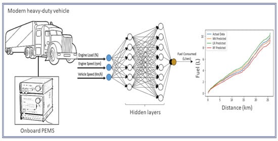
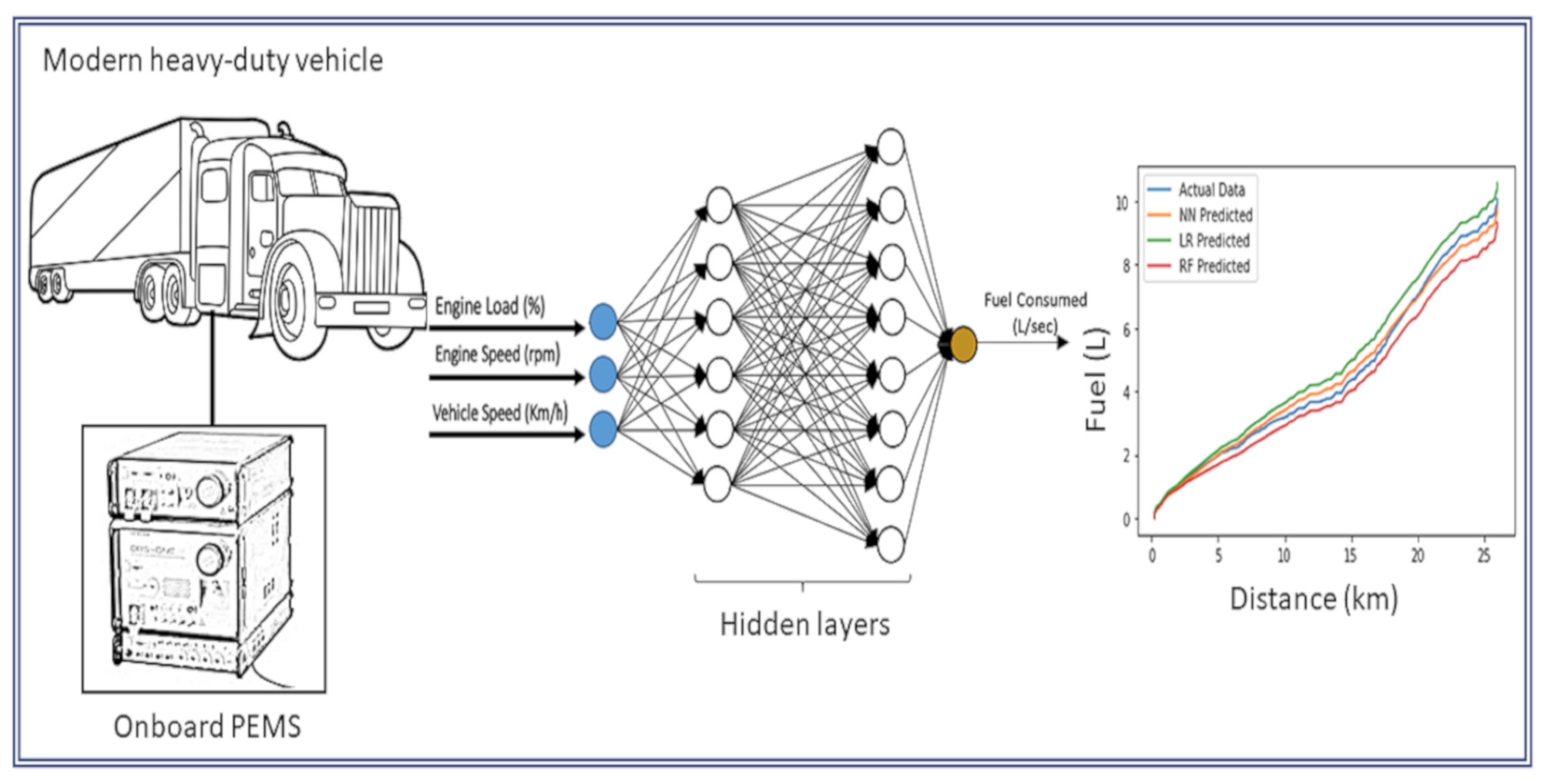
This current study models fuel consumption in modern heavy-duty trucks based on portable emissions monitoring system (PEMS) data collected during on-road testing. An artificial neural network was developed to predict the total fuel consumed by a vehicle on a trip based on very few key parameters, such as engine load (%), engine speed (rpm), and vehicle speed (km/h). The model also provides the trend in fuel consumption for the trip, which give insights into the diagnostic performance of the truck affected by the input parameters. The model can predict the total fuel consumed more accurately with a mean absolute error of 0.0014 and root mean square error of 0.0025 compared to other techniques such as linear regression [32] and random forest [20].

Table 1. Comparison of research results from previous studies.

Predicted Variable	Input Parameters	Method (Hidden Neurons Per Layer)	Result	Reference
Fuel Consumption in passenger cars	Cubic Capacity, Quantity of cylinders, Quantity of valves, Maximum Power, Maximum Torque, Compression Rate, Kerb Weight of Vehicle, Type of Engine, Fuel Injection, Type of charge, Gearbox, Drivetrain.	ANN (22-10-3) ANN (20-10-3)	R2 ≥ 0.98; RMSE = 5–8% R2 ≥ 0.98; RMSE = 6–10%	[23]
Fuel Consumption in trucks	Road Gradient, Torque% at the start, Torque% at the end, Average Acceleration, Gross Vehicle Weight, Road curvature radius, Longitudinal Profile Variance at 3 m, Longitudinal Profile Variance at 10 m, Longitudinal Profile Variance at 30 m, Vehicle Speed, Cruise control, Used Gear.	SVM RF ANN	R2 = 0.83; RMSE = 5.12; MAE = 3.56 R2 = 0.87; RMSE = 4.64; MAE = 3.21 R2 = 0.85; RMSE = 4.88; MAE = 3.46	[24]
Fuel Consumption based on floating vehicle data	Driver Gender, Driver Age, Transmission Type, Fuel Type, Weight, Mileage, Speed, Time, Location	ANN (9-4-1) ANN (9-6-1) ANN (9-8-1) ANN (9-10-1) ANN (9-12-1)	MSE = 0.00032692 MSE = 0.00037202 MSE = 0.00019523 MSE = 0.00009996 MSE = 0.00025849	[33]
Brake Specific Fuel Consumption and Exhaust Temperature in Diesel Engine	Engine Speed, Brake Mean Effective Pressure, Injection Timing.	ANN (3-7-2)	Mean Relative Error for BSFC = 1.93% Mean Relative Error for Exhaust Temperature = 2.36	[34]
Fuel Consumption	Engine Size, Distance, Fuel Type, Speed, Weight.	Radial Basis Function Neural Network (RBFNN) (5-15-1)	Maximum Error Percentage = 0.024 Absolute Average Error = 0.022071	[35]

Table 1. Comparison of research results from previous studies.

Predicted Variable	Input Parameters	Method (Hidden Neurons Per Layer)	Result	Reference
Fuel Consumption in passenger cars	Cubic Capacity, Quantity of cylinders, Quantity of valves, Maximum Power, Maximum Torque, Compression Rate, Kerb Weight of Vehicle, Type of Engine, Fuel Injection, Type of charge, Gearbox, Drivetrain.	ANN (22-10-3) ANN (20-10-3)	R2 ≥ 0.98; RMSE = 5–8% R2 ≥ 0.98; RMSE = 6–10%	[23]
Fuel Consumption in trucks	Road Gradient, Torque% at the start, Torque% at the end, Average Acceleration, Gross Vehicle Weight, Road curvature radius, Longitudinal Profile Variance at 3 m, Longitudinal Profile Variance at 10 m, Longitudinal Profile Variance at 30 m, Vehicle Speed, Cruise control, Used Gear.	SVM RF ANN	R2 = 0.83; RMSE = 5.12; MAE = 3.56 R2 = 0.87; RMSE = 4.64; MAE = 3.21 R2 = 0.85; RMSE = 4.88; MAE = 3.46	[24]
Fuel Consumption based on floating vehicle data	Driver Gender, Driver Age, Transmission Type, Fuel Type, Weight, Mileage, Speed, Time, Location	ANN (9-4-1) ANN (9-6-1) ANN (9-8-1) ANN (9-10-1) ANN (9-12-1)	MSE = 0.00032692 MSE = 0.00037202 MSE = 0.00019523 MSE = 0.00009996 MSE = 0.00025849	[33]
Brake Specific Fuel Consumption and Exhaust Temperature in Diesel Engine	Engine Speed, Brake Mean Effective Pressure, Injection Timing.	ANN (3-7-2)	Mean Relative Error for BSFC = 1.93% Mean Relative Error for Exhaust Temperature = 2.36	[34]
Fuel Consumption	Engine Size, Distance, Fuel Type, Speed, Weight.	Radial Basis Function Neural Network (RBFNN) (5-15-1)	Maximum Error Percentage = 0.024 Absolute Average Error = 0.022071	[35]

2. Methodology

Regression analysis was performed using Machine Learning techniques such as Artificial Neural Network, Linear Regression, and Random Forest to estimate the fuel consumption of modern heavy-duty trucks using PEMS data. The preprocessed dataset, which related to a single vehicle, contained 672,658 rows of actual torque (Nm), vehicle speed (km/h), and engine speed (rpm), which were used as inputs for the models. The implementation stages of the artificial neural network for fuel consumption modeling are as described:

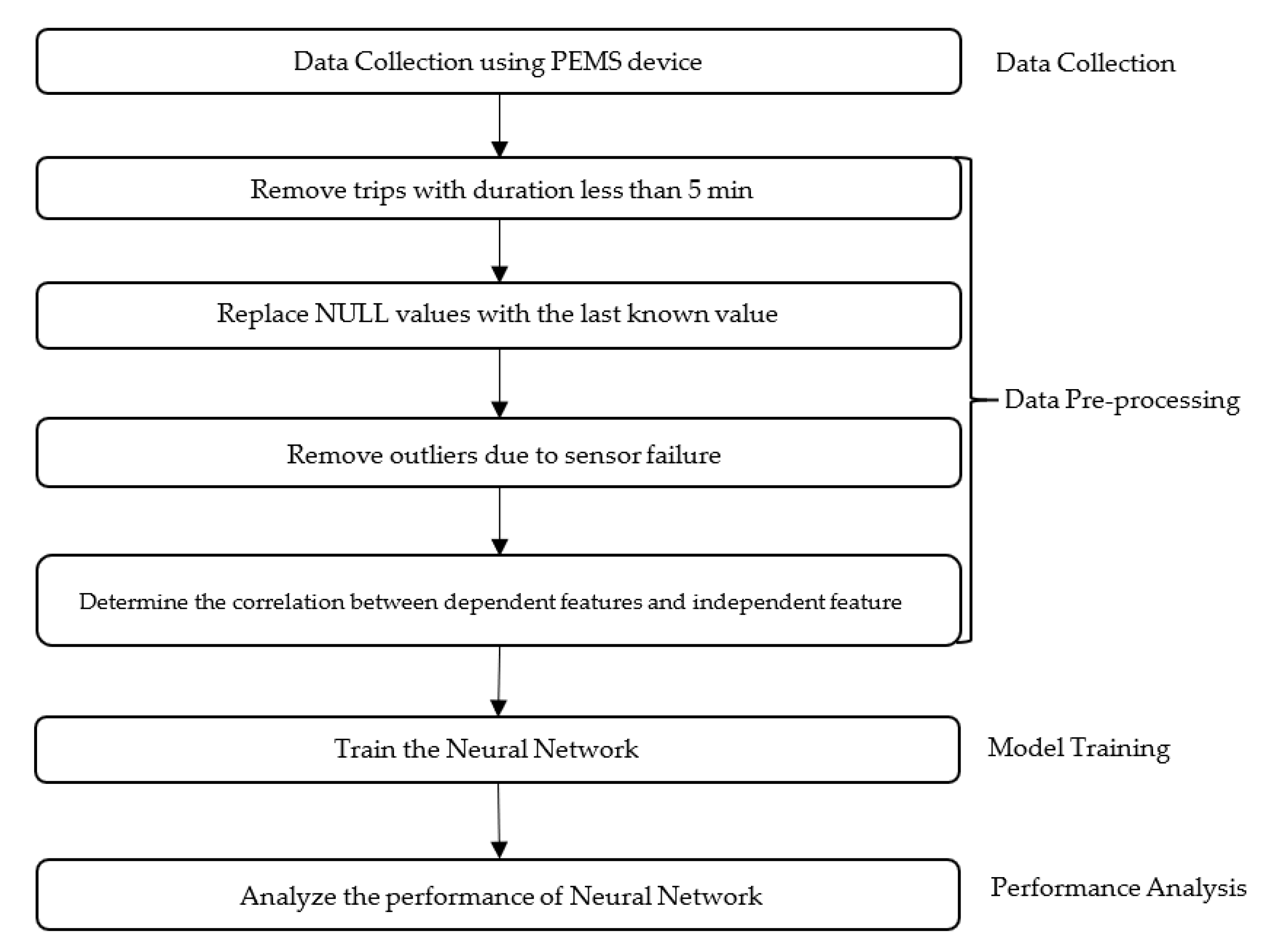
• Creating a database with data collected using PEMS devices during on-road testing of modern heavy-duty vehicles;
• Eliminating test trips that are less than 5 min duration as the trips may not capture information sufficient for the model to generalize well;
• Selecting the parameters that affect the fuel consumption based on parameters collected and domain knowledge;
• Performing correlation analysis on the input parameters selected to eliminate multi-collinear variables;
• Developing the neural networks and identifying the network with best-performing hyperparameters. The hyperparameters include the number of hidden layers, number of hidden neurons per layer, learning rate, and optimization function;
• Calculating the correlation coefficient on the reduced database using the best-performing model selected;
• Perform the generalization analysis of the model by calculating the performance measures such as MAE, RMSE, and R²;
• Evaluating the performance of the model by comparing the predicted values with the actual values collected during on-road testing.

Figure 1 shows the overall workflow for this work.

2.1. Data Collection and Pre-Processing

Data collection methods such as onboard emission measurement [36], laboratory measurement, and tunnel study [37] have been used in past. An on-road data collection method using PEMS is increasingly being used, which makes it possible to collect real-world fuel consumption and emission data [38], and has proved to be reliable [39]. The data used in the current study was collected using a PEMS device mounted on the vehicle during on-road testing at a frequency of 1Hz. PEMS software outputs for the sensor ports were used to process second by second data into a comma-separated values (CSV) file for each trip. Over 100 parameters such as fuel rate (L/h), engine speed (rpm), speed (km/h), gas temperature, CO₂, NOx, GPS altitude, GPS longitude, GPS latitude, etc. were collected for each trip based on data logger settings. Data were collected from two modern heavy-duty trucks with the same make/model of diesel engine manufactured in Detroit in 2016 were used in this study. The trucks were Cascadia models manufactured by Freightliner with DD13 engines and used as goods movement trucks. The on-road tests were performed in California, the fuel consumption during these on-road tests were recorded, and the cumulative fuel consumed per trip was calculated by summing the values. The vehicles were tested for multiple on-road trips with different routes, drivers, and conditions. However, modeling with too many parameters might overfit the ANN model resulting in poor performance. Hence, a subset of 10 features based on previous studies and domain knowledge was selected. These features included trip number, engine speed (rpm), trip distance (km), vehicle speed (km/h), fuel temperature (°C), fuel rate (L/s), accelerator pedal position (%), actual torque (Nm), power (kW), and engine load (%).

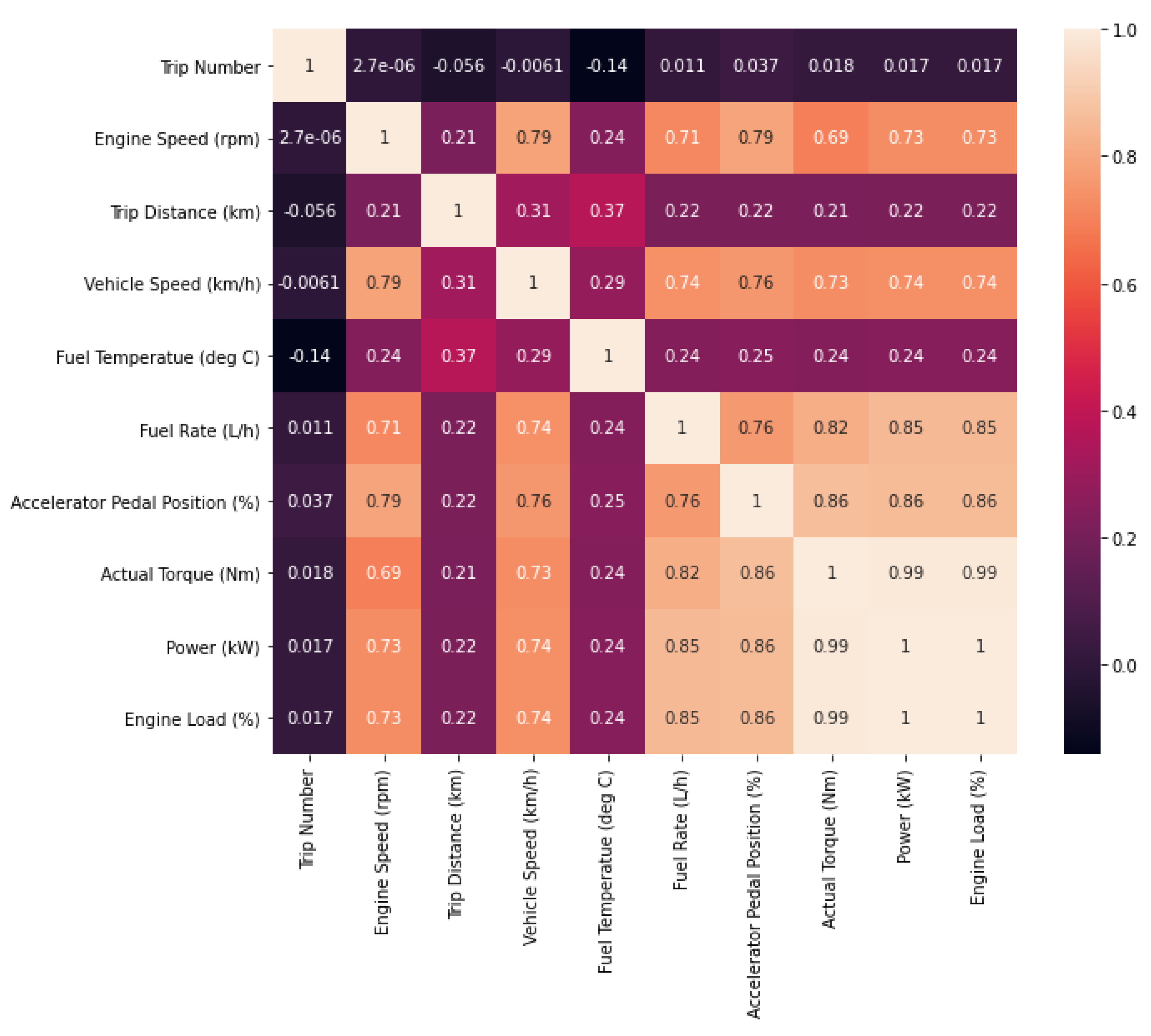
For better modeling of the neural network, the data collected must be representative. The raw dataset contains noise/missing values, redundant values, and outliers due to failure in the sensor or the sensor not having been enabled for recording. With feature engineering, the raw data is transformed into features that better represent the relation between features to the predictive model, resulting in better performance accuracy. The interpretation of the regression model is complex when independent variables are multi-collinear. Highly correlated independent variables overfit the model as a change in one variable causes significant change to another. Hence, to identify the multi-collinear variables, a correlation matrix that determines the correlation coefficient of each variable with every other variable in data is shown in Figure 2.

The last four rows and columns of the correlation matrix indicate that the independent features accelerator pedal position (%), actual torque (ft−lb), power (bhp), and engine load (%) are highly correlated to each other with a correlation coefficient of 0.85 and higher. Hence, to prevent overfitting of the model, only engine load (%) of the four parameters was used in modeling. Feature dimension can further be reduced by identifying the highly correlated features with the target variable fuel rate (L/s). The recursive feature elimination (RFE) method was used to identify and plot the feature importance scores. RFE determines the features based on the desired number by searching the subset of features starting with all features and recursively removing features. Feature importance of the remaining features, including engine load (%), accelerator pedal position (%), fuel temperature (deg C), vehicle speed (km/h), trip distance (km), and engine speed (rpm) concerning fuel rate (L/s), was determined with the RFE technique, and the top three features with the highest scores were selected for modeling. Based on the feature analysis, three independent features, namely engine load (%), vehicle speed (km/h), and engine speed (rpm), with high importance were selected for modeling the dependent feature fuel rate (L/s) and to identify patterns in fuel consumption.

2.2. Artificial Neural Network

Artificial neural networks is a machine learning technique inspired by biological neurons to create an accurate time-efficient predictive model [40]. ANN consists of multiple neurons which are computational, and the connections between neurons determine the functionality of the network [41]. The building block for a neural network is a neuron that represents the weighted sum of inputs passed through a non-linear activation function. The multi-layer perceptron (MLP) network is a type of neural network that consists of the input layer, one or more hidden layers, and an output layer. The initial layer takes the parameters/features as inputs to the network. At least one hidden layer is used to perform computations on input data by applying a non-linear activation function. The final output layer displays the output based on the task the network is trained for. ANN has gained popularity due to its adaptive learning ability and approximating non-linear functions to make predictions [42]. 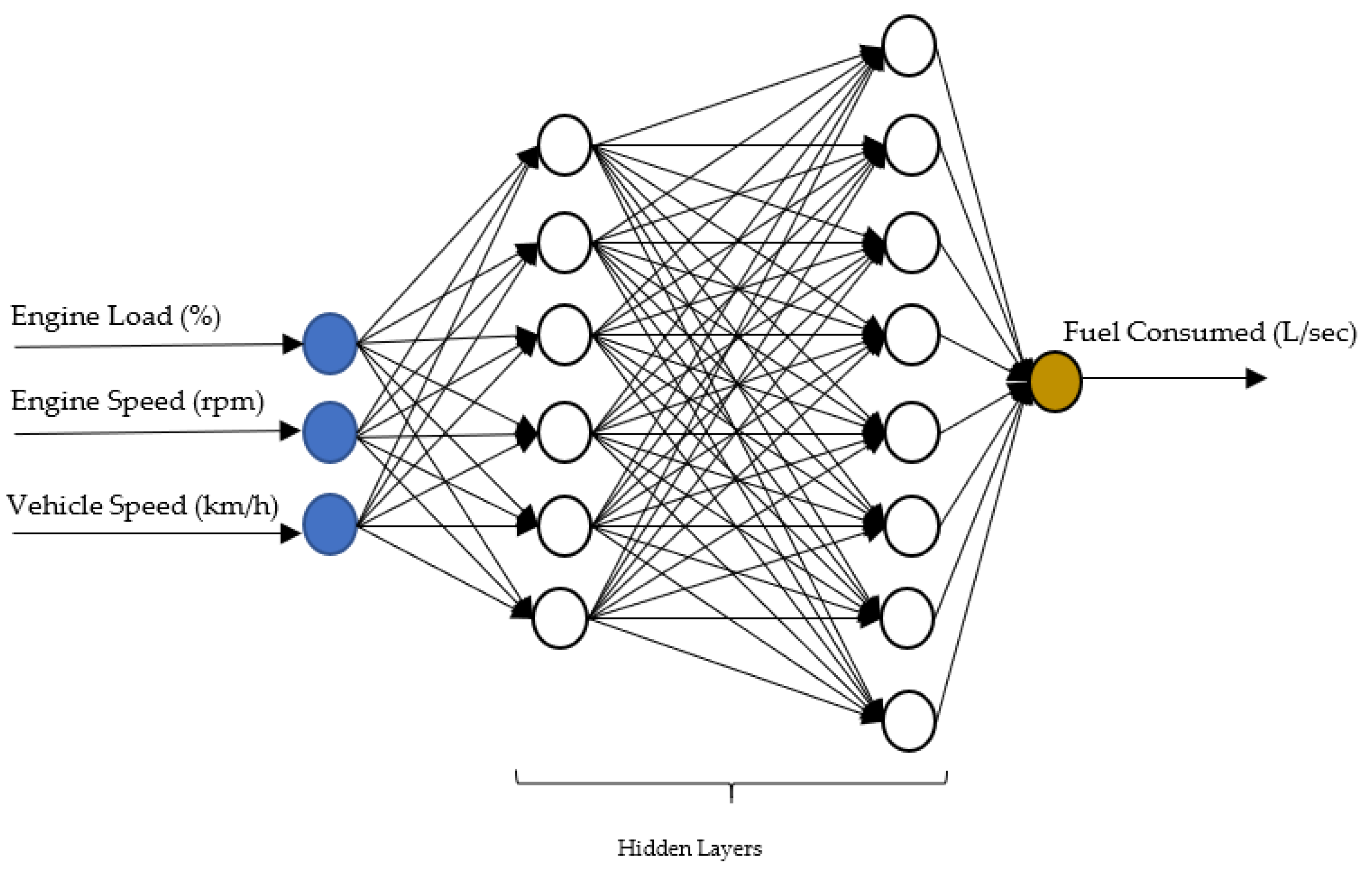In this study, a feed-forward neural network [43] where data is transmitted from the input layer to output layer in a forward direction assigning weights to the connection between layers with a backpropagation algorithm [44], ReLU [45] activation, and the mean square error function, was used. The backpropagation algorithm is a learning method used to optimize the weights of neurons in a neural network by repeatedly adjusting the weights to minimize the error of prediction. The network used for this work has three inputs to the input layers, two hidden layers with six and eight neurons in the respective layers, and an output layer with a single neuron as shown in Figure 3.

The available dataset of vehicle 1 was divided into train and test sets, with 70% to train the network, and 30% as a validation dataset, to test the generalization of the network [46]. The trained model weights were then used to make predictions on unseen test data (a single trip from vehicle 2). The performance of a neural network depends on many hyperparameters like the learning rate, number of epochs for training, initial weights, number of hidden layers, and the number of neurons in hidden layers. Multiple experiments were performed with different hyperparameters and the best results for the optimal network are presented in the results section.

2.3. Multiple Linear Regression

Linear Regression (LR) is the most well-known regression technique where the data is fitted to a straight line to predict output by minimizing a cost function or error. In this study, a multivariable linear equation given by Equation (1) is used due to multiple input parameters.

$$y={\theta }_0+{\theta }_1{x}_1+{\theta }_2{x}_2+{\theta }_3{x}_3$$

(1)

where, $y$ is the output and $x_1, x_2, x_3$ are the input variables with ${\theta }_0, {\theta }_{1, } {\theta }_2, {\theta }_3$ being parameters to learn.

2.4. Random Forest

Random Forest (RF) is an ensemble machine learning method for regression and classification tasks. This method uses many decision trees, and the outcome is based on predictions of these decision trees. Thus, the accuracy of the model can be improved by increasing the number of trees, making it robust to outliers. In this study, the random forest was trained with 100 trees, as the performance with more than 100 trees did not significantly improve accuracy and is computationally expensive.

3. Performance Measures

The performance of the machine learning model for the regression problem was evaluated using Mean Absolute Error (MAE), Root Mean Square Error (RMSE), and R-Squared (R²).

3.1. Mean Absolute Error

Mean Absolute Error (MAE) is the measure of error between the predicted value and the actual value given by Equation (2).

$$\mathrm{MAE}=\frac{1}{N}{\displaystyle \sum }_{t=1}^N|y_{pred,t}-y_{actual,t}|$$

(2)

where, $y_{pred,t}$ is the predicted value and $y_{actual,t}$ is the measured fuel consumption at the same instant of time.

3.2. Root Mean Squared Error

Root Mean Squared Error (RMSE) is the square root of the average squared difference between the predicted value and the actual value given by Equation (3). The smaller the value, the closer the predicted values to actual values.

$$\mathrm{RMSE}=\sqrt{\frac{1}{N}{\displaystyle \sum }_{t=1}^N{(\widehat{y}-y)}^2}$$

(3)

where, $\widehat{y}$ is the predicted value and $y$ is the measured fuel consumption at the same instant of time.

3.3. R-Squared

R-Squared (R²) is the statistical measure of variance for the dependent variable explained by the regression model given by Equation (4).

$$R^2=1-\frac{S{S}_{res}}{S{S}_{total}}$$

(4)

where, $S{S}_{res}$ is the sum of squares of residuals and $S{S}_{total}$ is the total sum of squares.

4. Results and Discussion

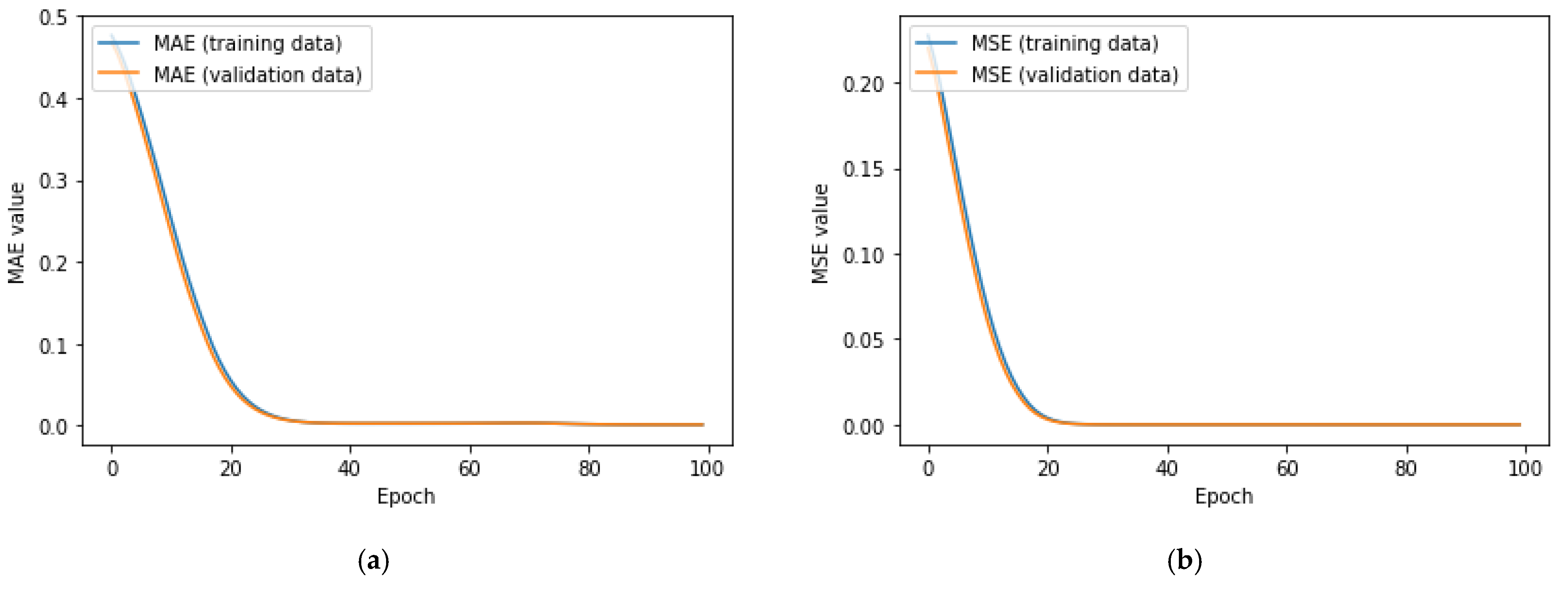
This study presents the fuel consumption modeling for modern heavy-duty vehicles using PEMS data under various driving conditions, different routes, and external factors. Engine Load (%), Engine Speed (rpm), and Vehicle Speed (km/h) were used as inputs for the ANN. Based on the hyper-parameter tuning, the neural network was trained for 100 epochs with a learning rate of 0.00001. During each epoch, the loss for each data item/batch in the training dataset and validation dataset was calculated. The loss plots shown in Figure 4 indicate the mean absolute error (MAE) and mean square error (MSE) on both training data and validation data.

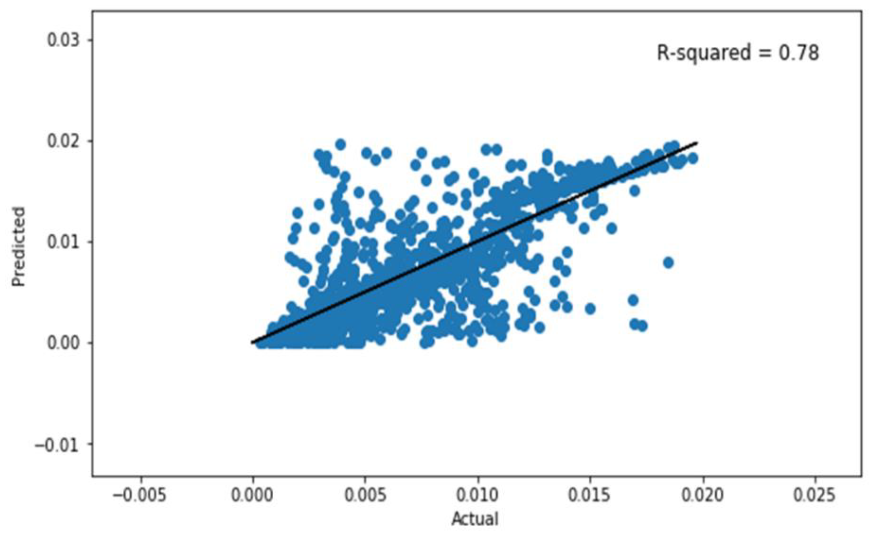
The minimum generalization gap of training and validation data loss plots indicates a good fit. The generalization of the neural network was tested on test data collected from a single trip of another vehicle. From Figure 5, the data points close to the line indicate the neural network model can accurately predict the fuel consumption with few outliers. The points far away from the regression line indicate outliers in data that were not captured by the neural network due to sudden transitions in vehicle speed (km/h) and engine speed (rpm) where fuel consumption was high.

To determine the total fuel consumed by vehicle, the cumulative fuel consumption was calculated by adding the instantaneous fuel rate values for every second. The performance measures described in Section 3 were used to evaluate the model and the values obtained are MAE: 0.0009, RMSE: 0.0021 for the training data. The R² value of 0.7806 on the test data and 0.7762 on the train data indicate that the neural network model is generalized well for unseen data.

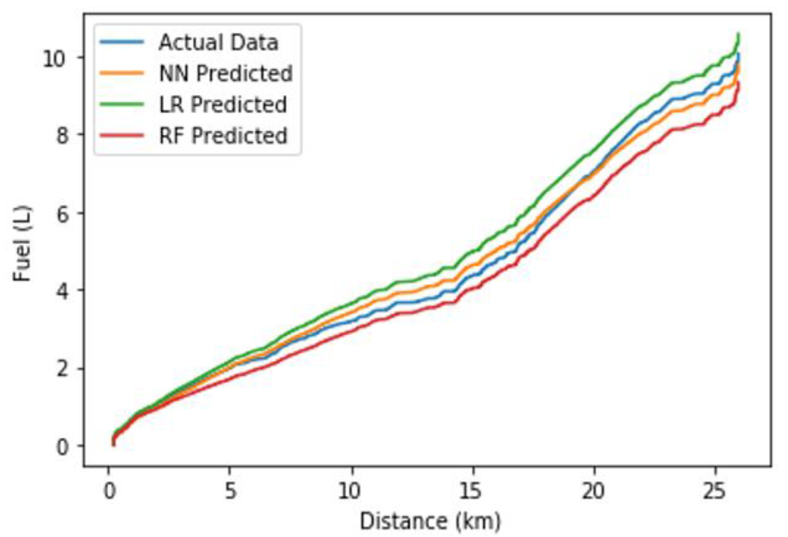
The cumulative fuel consumption with distance was plotted against the actual data to determine how well the neural network predicted total fuel consumption. To evaluate the performance, the neural network predictions were compared with predictions of linear regression and random forest. The performance metrics MAE, RMSE, R² are compared in

Table 2. Comparison of performance on test dataset.

Model	MAE	RMSE	R2	Fuel Consumed (L) (Measured)	Fuel Consumed (L) (Predicted)	$\%\mathbf{Error}=(\frac{\mathbf{Measured}-\mathbf{Predicted}}{\mathbf{Measured}})$
Artificial Neural Network (3-6-8-1)	0.0014	0.0025	0.7806	10.05	10.05	0
Linear Regression	0.0018	0.0029	0.7340	10.05	10.57	−0.05
Random Forest	0.0018	0.0030	0.7210	10.05	9.55	0.04

. Figure 6 shows the plots for comparison of cumulative fuel consumed for distance traveled for all models. The neural network prediction was closer to the actual measured data when compared to the linear regression model, which overestimated, and random forest, which underestimated the cumulative fuel consumed. The neural network model is better compared with other models because of its ability to predict values close to actual values. Also, the neural network model can be fine-tuned without developing a new model to perform the same task for complex learning on other vehicle types.

Based on the input features that were modeled it is easy to determine the parameter affecting the fuel consumption in case of anomaly. This study presents an efficient and practical method of estimating fuel consumption per trip, based on very few parameters for which data is easily available. The cost incurred in modeling the data is very low compared with other simulation methods that also consume more time.

5. Conclusions

In conclusion, the study demonstrates the modeling of fuel consumption in modern heavy-duty vehicles with an artificial neural network using very few technical parameters. An attempt was made to develop a model using very few parameters collected under different conditions. Data from modern heavy-duty trucks with the same make and model, driven by different persons on various routes under different external conditions, were used for training the artificial neural network. The model relies on very few parameters that could be obtained quickly and easily from a vehicle during a trip, unlike other parameters such as road grade, latitude, longitude, traffic information, etc. Moreover, the three parameters used were able to capture a minimum of 78% of the variance in the fuel rate compared to other studies where many parameters are used. Adding more input parameters would improve the performance of ANN, but collecting such data might require additional equipment setup. The performance measures MAE, RMSE, and R² indicate that accurate prediction can be obtained with the model. The data modeling can help to identify the trend in instantaneous fuel consumption and to calculate the total fuel consumed by the vehicle for each trip, which can further help in diagnosing vehicle performance in the case of abnormalities. Models that are accurate, fast, and able to predict in real-time will enable the optimization of fuel consumption. The model can be fine-tuned easily to model more complex data from other vehicles with different makes and models that do not have the amount on-road data needed to train a network. This work can be extended to include other factors such as time, traffic information, road information, GPS data, etc. that affect fuel consumption, and to estimate vehicle exhaust emissions.

References

- Zhu, D.; Zheng, X. Fuel consumption and emission characteristics in an asymmetric twin-scroll turbocharged diesel engine with two exhaust gas recirculation circuits. Appl. Energy 2019, 238, 985–995. [Google Scholar] [CrossRef]
- Wang, J.; Rakha, H.A. Fuel consumption model for conventional diesel buses. Appl. Energy 2016, 170, 394–402. [Google Scholar] [CrossRef]
- Hellström, E.; Ivarsson, M.; Åslund, J.; Nielsen, L. Look-ahead control for heavy trucks to minimize trip time and fuel consumption. Control Eng. Pract. 2009, 17, 245–254. [Google Scholar] [CrossRef] [Green Version]
- Lo, C.-L.; Chen, C.-H.; Kuan, T.-S.; Lo, K.-R.; Cho, H.-J. Fuel Consumption Estimation System and Method with Lower Cost. Symmetry 2017, 9, 105. [Google Scholar] [CrossRef] [Green Version]
- Agency, E.P. Sources of Greenhouse Gas Emissions. Available online: https://www.epa.gov/ghgemissions/sources-greenhouse-gas-emissions (accessed on 5 October 2021).
- NHTSA’s Corporate Average Fuel Economy (CAFE). Available online: https://www.nhtsa.gov/laws-regulations/corporate-average-fuel-economy (accessed on 5 October 2021).
- Anderson, S.T.; Fischer, C.; Parry, I.; Sallée, J.M. Automobile Fuel Economy Standards: Impacts, Efficiency, and Alternatives. Rev. Environ. Econ. Policy 2011, 5, 89–108. [Google Scholar] [CrossRef] [Green Version]
- U.S. Environmental Protection Agency. Greenhouse Gas Emissions and Fuel Efficiency Standards for Medium- and Heavy-Duty Engines and Vehicles-Phase 2; Regulatory Impact Analysis EPA-420-R-16-900; Office of Transportation and Air Quality: Ann Arbor, MI, USA, 2016.
- Nasser, S.H.; Weibermel, V.; Wiek, J. Computer Simulation of Vehicle’s Performance and Fuel Consumption under Steady and Dynamic Driving Conditions; SAE Technical Paper 981089; SAE: Warrendale, PA, USA, 1998; p. 16. [Google Scholar] [CrossRef]
- Cappiello, A.; Chabini, I.; Nam, E.K.; Lue, A.; Abou Zeid, M. A statistical model of vehicle emissions and fuel consumption. In Proceedings of the IEEE 5th International Conference on Intelligent Transportation Systems, Singapore, 6 September 2002; pp. 801–809. [Google Scholar] [CrossRef] [Green Version]
- Giannelli, R.A.; Nam, E.K.; Helmer, K.; Younglove, T.; Scora, G.; Barth, M. Heavy-Duty Diesel Vehicle Fuel Consumption Modeling Based on Road Load and Power Train Parameters; SAE Technical Paper 2005-01-3549; SAE: Warrendale, PA, USA, 2005. [Google Scholar] [CrossRef] [Green Version]
- Bifulco, G.N.; Galante, F.; Pariota, L.; Spena, M.R. A Linear Model for the Estimation of Fuel Consumption and the Impact Evaluation of Advanced Driving Assistance Systems. Sustainability 2015, 7, 14326–14343. [Google Scholar] [CrossRef] [Green Version]
- Yao, Y.; Zhao, X.; Zhang, Y.; Chen, C.; Rong, J. Modeling of individual vehicle safety and fuel consumption under comprehensive external conditions. Transp. Res. Part D Transp. Environ. 2020, 79, 10024. [Google Scholar] [CrossRef]
- Ivkovic, I.; Kaplanović, S.; Milovanović, B. Influence of road and traffic conditions on fuel consumption and fuel cost for different bus technologies. Therm. Sci. 2017, 21, 693–706. [Google Scholar] [CrossRef] [Green Version]
- Ma, H.; Xie, H.; Huang, D.; Xiong, S. Effects of driving style on the fuel consumption of city buses under different road conditions and vehicle masses. Transp. Res. Part D Transp. Environ. 2015, 41, 205–216. [Google Scholar] [CrossRef]
- Tzirakis, E.G.; Zannikos, F.E.; Stournas, S. Impact of driving style on fuel consumption and exhaust emissions: Defensive and aggressive driving style. In Proceedings of the 10th International Conference on Environmental Science and Technology Kos Island, Kos Island, Greece, 5–7 September 2007. [Google Scholar]
- Jeon, H. The Impact of Climate Change on Passenger Vehicle Fuel Consumption: Evidence from U.S. Panel Data. Energies 2019, 12, 4460. [Google Scholar] [CrossRef] [Green Version]
- Shang, R.; Zhang, Y.; Max Shen, Z.-J.; Zhang, Y. Analyzing the Effects of Road Type and Rainy Weather on Fuel Consumption and Emissions: A Mesoscopic Model Based on Big Traffic Data. IEEE Access 2021, 9, 62298–62315. [Google Scholar] [CrossRef]
- Cortes, C.; Vapnik, V. Support-vector networks. Mach. Learn. 1995, 20, 273–297. [Google Scholar] [CrossRef]
- Breiman, L. Random Forests. Mach. Learn. 2001, 45, 5–32. [Google Scholar] [CrossRef] [Green Version]
- McCulloch, W.S.; Walter, P. A Logical Calculus of Ideas Immanent in Nervous Activity. Bull. Math. Biophys. 1990, 5, 115–133. [Google Scholar] [CrossRef]
- Rosenblatt, F. The Perceptron: A Probabilistic Model for Information Storage and Organization in the Brain. Psychol. Rev. 1958, 65, 386–408. [Google Scholar] [CrossRef] [Green Version]
- Ziółkowski, J.; Oszczypała, M.; Małachowski, J.; Szkutnik-Rogoż, J. Use of Artificial Neural Networks to Predict Fuel Consumption on the Basis of Technical Parameters of Vehicles. Energies 2021, 14, 2639. [Google Scholar] [CrossRef]
- Perrotta, F.; Parry, T.; Neves, L. Application of machine learning for fuel consumption modeling of trucks. In Proceedings of the IEEE International Conference on Big Data (Big Data), Orlando, FL, USA, 5 September 2021; pp. 3810–3815. [Google Scholar] [CrossRef]
- Kim, Y.-R.; Jung, M.; Park, J.-B. Development of a Fuel Consumption Prediction Model Based on Machine Learning Using Ship In-Service Data. J. Mar. Sci. Eng. 2021, 9, 137. [Google Scholar] [CrossRef]
- Baumann, S.; Neidhardt, T.; Klingauf, U. Evaluation of the aircraft fuel economy using advanced statistics and machine learning. CEAS Aeronaut J. 2021, 12, 669–681. [Google Scholar] [CrossRef]
- Wang, H.; Fu, L.; Zhou, Y.; Li, H. Modelling of the fuel consumption for passenger cars regarding driving characteristics. Transp. Res. Part D Transp. Environ. 2008, 13, 479–482. [Google Scholar] [CrossRef]
- Zeng, I.Y.; Tan, S.; Xiong, J.; Ding, X.; Li, Y.; Wu, T. Estimation of Real-World Fuel Consumption Rate of Light-Duty Vehicles Based on the Records Reported by Vehicle Owners. Energies 2021, 14, 7915. [Google Scholar] [CrossRef]
- Schoen, A.; Byerly, A.; Hendrix, B.; Bagwe, R.M.; Santos, E.C.d.; Miled, Z.B. A Machine Learning Model for Average Fuel Consumption in Heavy Vehicles. IEEE Trans. Veh. Technol. 2019, 68, 6343–6351. [Google Scholar] [CrossRef] [Green Version]
- Zhou, M.; Jin, H.; Wang, W. A review of vehicle fuel consumption to evaluate eco-driving and eco-routing. Transp. Res. Part D Transp. Environ. 2016, 49, 203–218. [Google Scholar] [CrossRef]
- Zacharof, N.; Fontaras, G.; Ciuffo, B.; Tsiakmakis, S. Review of in Use Factors Affecting the Fuel Consumption and CO2 Emissions of Passenger Cars; EUR 27819 EN; Publications Office of the European Union: Luxembourg, 2016. [Google Scholar] [CrossRef]
- Freedman, D.A. Statistical Models: Theory and Practice; Cambridge University Press: Cambridge, UK, 2009; p. 26. [Google Scholar]
- Du, Y.; Wu, J.; Yang, S.; Zhou, L. Predicting vehicle fuel consumption patterns using floating vehicle data. J. Environ. Sci. 2017, 59, 24–29. [Google Scholar] [CrossRef]
- Parlak, A.; İslamoğlu, Y.; Yasar, H.; Egrisogut, A. Application of Artificial Neural Network to Predict Specific Fuel Consumption and Exhaust Temperature for a Diesel Engine. Appl. Therm. Eng. 2006, 824–828. [Google Scholar] [CrossRef]
- Amer, A.; Abdalla, A.; Noraziah, A.; Fauzi, A.A.C. Prediction of Vehicle Fuel Consumption Model Based on Artificial Neural Network. Appl. Mech. Mater. 2014, 492, 3–6. [Google Scholar] [CrossRef]
- Barth, M.; An, F.; Younglove, T.; Scora, G.; Levine, C.; Ross, M.; Wenzel, T. Comprehensive Modal Emission Model (CMEM), Version 2.0, User’s Guide; University of California: Riverside, CA, USA, 2000. [Google Scholar]
- John, C.; Friedrich, R.; Staehelin, J.; Schläpfer, K.; Stahel, W.A. Comparison of emission factors for road traffic from a tunnel study (Gubrist tunnel, Switzerland) and from emission modeling. Atmos. Environ. 1999, 33, 3367–3376. [Google Scholar] [CrossRef]
- Song, G.; Yu, L.; Zhang, X. Emission Analysis at Toll Station Area in Beijing with Portable Emission Measurement System. Transp. Res. Rec. 2008, 2058, 106–114. [Google Scholar] [CrossRef]
- Liu, H.; Barth, M.; Scora, G.; Davis, N.; Lents, J. Using Portable Emission Measurement System for Transportation Emissions Studies: Comparison with Laboratory Methods. In Proceedings of the 89th Transportation Research Board Annual Meeting, Washington, DC, USA, January 2010; Volume 2158, pp. 1–9. [Google Scholar] [CrossRef]
- Karlaftis, M.G.; Vlahogianni, E.I. Statistical Methods versus Neural Networks in Transportation Research: Differences, Similarities and Some Insights. Transp. Res. Part C Emerg. Technol. 2011, 19, 387–399. [Google Scholar] [CrossRef]
- Park, Y.-S.; Lek, S. Chapter 7-Artificial Neural Networks: Multilayer Perceptron for Ecological Modeling. Dev. Environ. Model. 2016, 28, 123–140. [Google Scholar] [CrossRef]
- Lippmann, R. An introduction to computing with neural nets. IEEE ASSP Mag. 1987, 4, 4–22. [Google Scholar] [CrossRef]
- Hornik, K.; Stinchcombe, M.; White, H. Multilayer feedforward networks are universal approximators. Neural Netw. 1989, 2, 359–366, 0893–6080. [Google Scholar] [CrossRef]
- Rumelhart, D.E.; Hinton, G.E.; Williams, R.J. Learning representations by backpropagation error. Nature 1986, 323, 533–536. [Google Scholar] [CrossRef]
- Brownlee, J. A Gentle Introduction to the Rectified Linear Unit (ReLU); Machine Learning Mastery: San Juan, PR, USA, 2019; Retrieved 8 April 2021. [Google Scholar]
- Haykin, S. Neural Networks, A Comprehensive Foundation; McMillian College Publishing Company: New York, NY, USA, 1994. [Google Scholar]