Article

Well-Logging Prediction Based on Hybrid Neural Network Model

Petroleum Engineering Department, Xi’an Shiyou University, Xi’an 710065, China
*
Authors to whom correspondence should be addressed.
Energies 2021, 14(24), 8583; https://doi.org/10.3390/en14248583
Submission received: 12 November 2021 / Revised: 10 December 2021 / Accepted: 14 December 2021 / Published: 20 December 2021
(This article belongs to the Special Issue Application of Machine Learning in Rock Characterization)

Abstract

:
Well-logging is an important formation characterization and resource evaluation method in oil and gas exploration and development. However, there has been a shortage of well-logging data because Well-logging can only be measured by expensive and time-consuming field tests. In this study, we aimed to find effective machine learning techniques for well-logging data prediction, considering the temporal and spatial characteristics of well-logging data. To achieve this goal, the convolutional neural network (CNN) and the long short-term memory (LSTM) neural networks were combined to extract the spatial and temporal features of well-logging data, and the particle swarm optimization (PSO) algorithm was used to determine hyperparameters of the optimal CNN-LSTM architecture to predict logging curves in this study. We applied the proposed CNN-LSTM-PSO model, along with support vector regression, gradient-boosting regression, CNN-PSO, and LSTM-PSO models, to forecast photoelectric effect (PE) logs from other logs of the target well, and from logs of adjacent wells. Among the applied algorithms, the proposed CNN-LSTM-PSO model generated the best prediction of PE logs because it fully considers the spatio-temporal information of other well-logging curves. The prediction accuracy of the PE log using logs of the adjacent wells was not as good as that using the other well-logging data of the target well itself, due to geological uncertainties between the target well and adjacent wells. The results also show that the prediction accuracy of the models can be significantly improved with the PSO algorithm. The proposed CNN-LSTM-PSO model was found to enable reliable and efficient Well-logging prediction for existing and new drilled wells; further, as the reservoir complexity increases, the proxy model should be able to reduce the optimization time dramatically.

1. Introduction

Well-logging is the process of characterizing the variations in physical properties of formations, such as electromagnetic, acoustic, nuclear radiation, and thermal energy, with depth along a borehole using specialized instrumentation. The interpretation and utilization of well-logging data is particularly important in petroleum engineering [1,2]. The conventional methods of well-logging interpretation are empirical and statistical models that establish the relationship between different rock properties and estimate missing log data using correlations [3].
The application of artificial intelligence (AI) in the field of well-logging is emerging and promising [4]. In recent years, more and more oilfield researchers are using deep learning techniques to predict different reservoir properties, such as permeability, porosity, and fluid saturation, from available well-logging data to reduce the cost of exploration and development. Researchers have proposed a series of algorithms with shallow-learning mechanisms [5,6,7]. However, these algorithms are only suitable for the application and theoretical analysis of specific-scale data, and their effect is not good for the application of large-sample data analysis or feature extraction from complex feature data. Hinton et al. [8] pointed out that deep neural networks have a dimensionality reduction effect on high-dimensional data and can characterize the target data well, which can alleviate the difficulties caused by the analysis and recognition of multidimensional massive data to a certain extent, and can become a bright spot of machine learning. Deep learning can represent data feature information at multiple levels; it can automatically abstract high-dimensional data at different levels to accomplish specific tasks [9].
Well-logging curve reconstruction refers to the data reconstruction of inappropriate parts of existing well-logging curves using correlated data or objective laws obtained from massive data. Because of the advantages of deep learning in feature extraction, previous studies have applied deep learning algorithms to predict the missing well-logging curves by inputting well-logging data and constructing a model with the help of algorithms to achieve the reconstruction of the target curve [10]. Korjani et al. [11] proposed a reservoir-modeling method based on deep neural networks for predicting petrophysical characteristics. They used a large amount of geological data from neighboring drilled wells to construct virtual logging data for well sections lacking well-logging curves and core data. Parapuram et al. [12] proposed a multistage curve generation scheme in which the well-logging curves generated in each stage automatically participate in the next stage to improve the accuracy of the final predicted well-logging curves. Yang et al. [
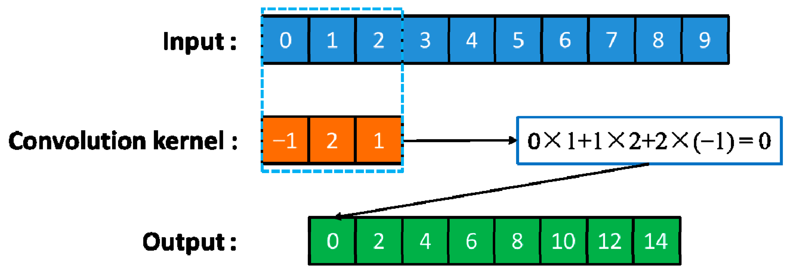
13] selected four logging parameters—compensation density, acoustic time difference, natural gamma, and mud content—as independent variables of a convolutional neural network (CNN) to reconstruct the variation curves of dependent variables, such as porosity. However, CNNs can only capture the spatial properties of a well-logging curve, and the properties of the rocks usually exhibit a trend with depth. In contrast, recurrent neural networks (RNNs) consider both internal and external inputs from the previous step and, thus, can capture the trend with depth [14]. Zhang et al. [
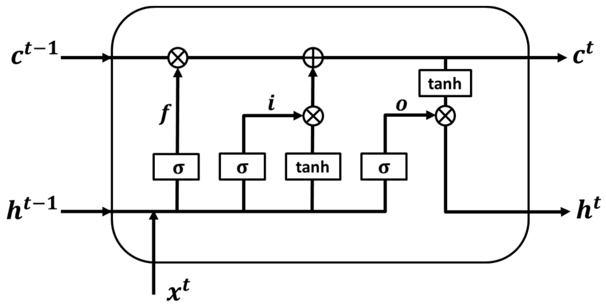
15] considered well-logging as a data sequence, and designed a long short-term memory (LSTM) network model to predict the entire well-logging curve or the missing well-logging curve. Pham et al. [16] integrated bidirectional LSTM (BiLSTM) with a fully connected neural network to generate accurate acoustic logs from neutron porosity logs, gamma ray logs, and density logs. Their proposed method combines the local shapes of well-logging curves with different geological profiles to improve the predictions.
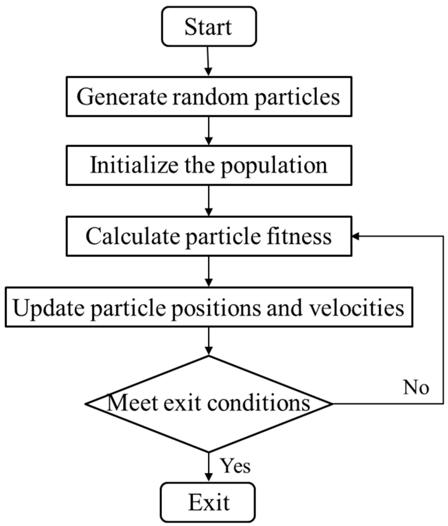
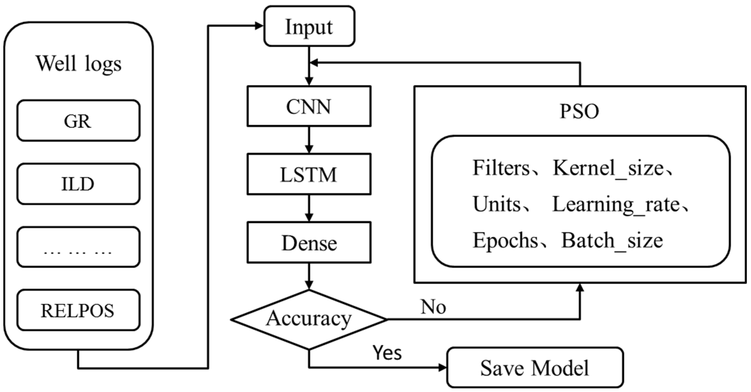
The focus of this study was on the use of machine learning techniques to solve the logging curve complementation and generation problem. Current research using machine learning methods to predict missing well-logging curves can rarely account for both the spatial and temporal characteristics of the logging data. To overcome the shortcomings, we proposed a new neural network architecture that was composed of CNN and LSTM, which respectively extracts the temporal and spatial characteristics of well-logging data to predict the well logs of interest. To further improve the prediction accuracy, the CNN-LSTM model was then optimized by the particle swarm optimization (PSO) algorithm, which is another new contribution of this study.
The main structure of this paper is as follows: Section 2 introduces the theoretical basis of the basic neural networks CNN, LSTM and PSO used in this study. Section 3 presents the architecture of the hybrid neural network model (CNN-LSTM-PSO), and describes the evaluation metrics used to evaluate the performance of the CNN-LSTM-PSO model. Section 4 presents the data source of the well-logging dataset, and performs PE log prediction from other logs of the target well and from logs of adjacent wells with the proposed CNN-LSTM-PSO model. Then, the superiority of the proposed model is evaluated by comparing it with other conventional machine learning methods, such as the SVR, GBDT, CNN-PSO and LSTM-PSO models. Section 5 summarizes the main problems of using current AI technologies in well-logging applications, and presents our future work. The conclusions are presented in Section 6.

2. Methodology

This section introduces the theoretical basis of the convolutional neural network (CNN), the long short-term memory neural network (LSTM), and particle swarm optimization (PSO) algorithms in detail.

2.1. Convolutional Neural Network

CNN is a feed-forward neural network that consists of an input layer, convolutional layer, pooling layer, fully connected layer, and output layer [17]. CNN obtains implicit features from the input data by performing convolutional and pooling operations and then fuses the extracted features into a fully connected layer to introduce the output of neurons using an activation function [18].
This study used a one-dimensional CNN structure, as shown in Figure 1, because the convolutional kernel is only scanned along the depth direction of the well-logging curve. The convolutional layer is the soul of CNNs, and they can be trained more deeply, accurately, and efficiently if they contain shorter connections between the layers closer to the input and the layers closer to the output [19]. The convolutional layer parameters include neuron perception domain size, sliding step size, and filling method, which together determine the size of the output features of the convolutional layer and are the hyperparameters of the CNN. CNNs usually use a rectified linear unit (ReLU) to generate the output of the convolutional layer [20]. The fully connected layer is equivalent to the implicit layer in a traditional feed-forward neural network, is located at the end of the implicit layer of the CNN, and only passes signals to the other fully connected layers.
The special feature of the CNN as a multilayer perceptron is the local perceptual field and weight-sharing method, which reduces the number of weights, thus making the network easier to optimize and reducing the risk of overfitting [21]. By simply sensing the local area and then synthesizing the local information at a higher level to get the global information, weight sharing means that the features learned in one part can also be used in another part while reducing the complexity of the network model. In CNNs, the alternating role of convolutional and pooling layers can mine deep features with differentiation from a large amount of data.

2.2. Long Short-Term Memory Neural Network

LSTM is a special kind of RNN proposed mainly to solve the gradient disappearance and gradient explosion problems in long time sequence training [22,23]. Compared with the traditional RNN, LSTM adds memory units to each neural unit in the hidden layer to control the memory information on the time sequence while each neural unit is passed through the gate structure (forgetting gate, input gate, and output gate). A typical network structure of LSTM is shown in Figure 2.
The forgetting gate selectively forgets the input passed from the previous node. Specifically, z f (f denotes forget) is calculated as the forgetting gate to control which c t 1 of the previous state needs to be left behind and which needs to be forgotten. The input gate takes the inputs of this stage and remembers them selectively. Mainly, it selectively memorizes the input, x t , recording more important parts and less unimportant ones. The current input is represented by the z obtained from the previous calculation. The selected gate signal is controlled by z i (i stands for information). The results obtained from the above two steps are summed to obtain the ct transmitted to the next state. ct is expressed as follows ( indicates vector fork multiplication):
c t = z f c t 1 + z i z
The output gate determines which will be output as the current state. The main control is achieved through z o , and the c o obtained in the previous stage is deflated (varied by a tanh activation function). Similar to a normal RNN, the output, y t , is often eventually obtained by h t variation, as follows:
h t = z o t a n h ( c t )
y t = σ ( W h t )  
As described above, the weights of each gate are obtained by continuously training the input data. The information of the output result h t of layer t of the model is used as the input information for the next layer of the model, and finally, the LSTM prediction model is obtained through a recursive process.

2.3. Particle Swarm Optimization

PSO is an evolutionary computational technique that originated as a simplified model of the population intelligence algorithm used in a study on the foraging behavior of birds [25,26]. The algorithm was originally inspired by the regularity of flocking activities of birds of prey, which in turn led to a simplified model using group intelligence to find the optimal solution through collaboration and information sharing among individuals in the population [27].
Figure 3 shows the process of the PSO algorithm, in which each particle individually searches for the optimal solution in the search space. The optimal solution is recorded as the current individual extreme value, and is shared with the other particles in the whole particle swarm. The particle travels at a certain speed in the search space, and the speed and position are dynamically adjusted according to its own flight experience and the flight experience of other particles [28]. Three simple rules can be summarized for particle swarm algorithms: (1) fly away from the nearest individual to avoid collision, (2) fly toward the target, and (3) fly toward the center of the population.
The equation to update particle velocity in the PSO algorithm is as follows:
V n e w = ω V i d + C 1 r a n d o m ( 0 , 1 ) ( P i d X i d ) + C 2 r a n d o m ( 0 , 1 ) ( P g d X i d )
where V i d is the current velocity of the particle; ω is the inertia factor (with velocity there is motion inertia); r a n d o m ( 0 , 1 ) is the random number generation function that generates random numbers between 0 and 1; P i d is the current position of the particle; X i d is the global best position of this particle; P g d represents the current best position among all particles in the population; and C1 and C2 denote the learning factors, which learn from the best position in the history of this particle and the best position in the population, respectively.
Other important parameters in PSO include velocity limit, V m a x , position limit, X m a x , population size, and initial population. Because of its simple operation and fast convergence, PSO has been widely used in science and engineering, such as function optimization, image processing, and geodesy [29].

3. CNN-LSTM-PSO Model and Evaluation Metrics

3.1. CNN-LSTM-PSO Model

Figure 4 shows the overall architecture to predict well-logging curves using the CNN-LSTM-PSO model proposed in this study. The CNN-LSTM-PSO network structure consists of a one-dimensional CNN, LSTM, and feature fusion layers. The CNN layer is responsible for capturing local trends and features of the well-logging data. The LSTM layer is responsible for learning short-term variation features of the well-logging data and long-term dependent periodic features. The feature fusion layer fuses different spatiotemporal features in the feature fusion layer. Then, these spatiotemporal features are used as inputs for prediction in the regression layer. Finally, the hyperparameters of the CNN-LSTM hybrid network are optimized by the PSO algorithm, mainly including filters and kernel_size of the CNN layer, units of the LSTM layer, and learning_rate, epochs, and batch_size [30]. The PSO algorithm is designed to find the optimal hyperparameter structure while moving the encoded particles, which is then applied to well-logging curve prediction.
The basic steps of the CNN-LSTM-PSO model are as follows:
  • Acquire the well-logging curve data. Then normalize and divide the data set to obtain the training sample data set and test data set of CNN-LSTM;
  • Train the CNN-LSTM model with the partitioned training sample data set, optimize the hyperparameters of the CNN-LSTM by the PSO algorithm, and test the performance of the model;
  • Save the best CNN-LSTM model, make predictions with the test data set, and compare it with traditional machine learning models, including support vector regression (SVR), gradient-boosting regression (GBDT), CNN, and LSTM models.

3.2. Evaluation Metrics

In the experiments, two commonly used predictive metrics, root mean square error (RMSE) and coefficient of determination (R2), were applied to evaluate the performance of log prediction results. These two evaluation metrics provide reference indicators for the prediction accuracy of the model. Lower RMSE values and higher R2 values indicate the better performance of the model [31,32].
The RMSE metric was calculated using the following equation:
R M S E = i = 1 n ( y i ^ y i ) 2 N
where y i ^ is the value predicted by the regression model, and N is the number of observations.
R2 is calculated by the following formula:
R 2 = 1 S S r e s S S t o t
where SSres is the residual sum of squares, and SStot is the total sum of squares, calculated by the following expression:
S S r e s = ( y i y r e g ) 2
S S t o t = ( y i y ¯ ) 2
where y i is the value of each data point, y ¯ is the mean value, and yreg is the value predicted by the regression model.

4. Experiments and Results

The main objective of this section is to evaluate the effectiveness of the CNN-LSTM-PSO model in predicting well-logging curves, as well as to compare the performance and accuracy of the neural network with traditional regression algorithms. All experiments were carried out on the Google Colab platform (1 December 2021, https://colab.research.google.com) using the Python 3.7 and TensorFlow 2.7 environment to implement the proposed network. Google Colab is a product developed by the Google Research team to write and execute arbitrary Python code through a browser, especially for machine learning and data analysis.

4.1. Experimental Data Set

The experimental data set of this study comprised public data downloaded from GitHub open-source collection of well-logging data (https://github.com/sunyingjian). In total, eight wells from a gas reservoir in Cornwall, Kansas, were included in the data set. Each well contained seven logging attributes, including natural gamma ray, resistivity, photoelectric effect, neutron density–porosity difference, average of neutron and density logs, nonmarine–marine indicator, and relative position. The data set was divided into training and validation sets using a ratio of 80:20 to evaluate the performance of the CNN-LSTM-PSO model architecture.
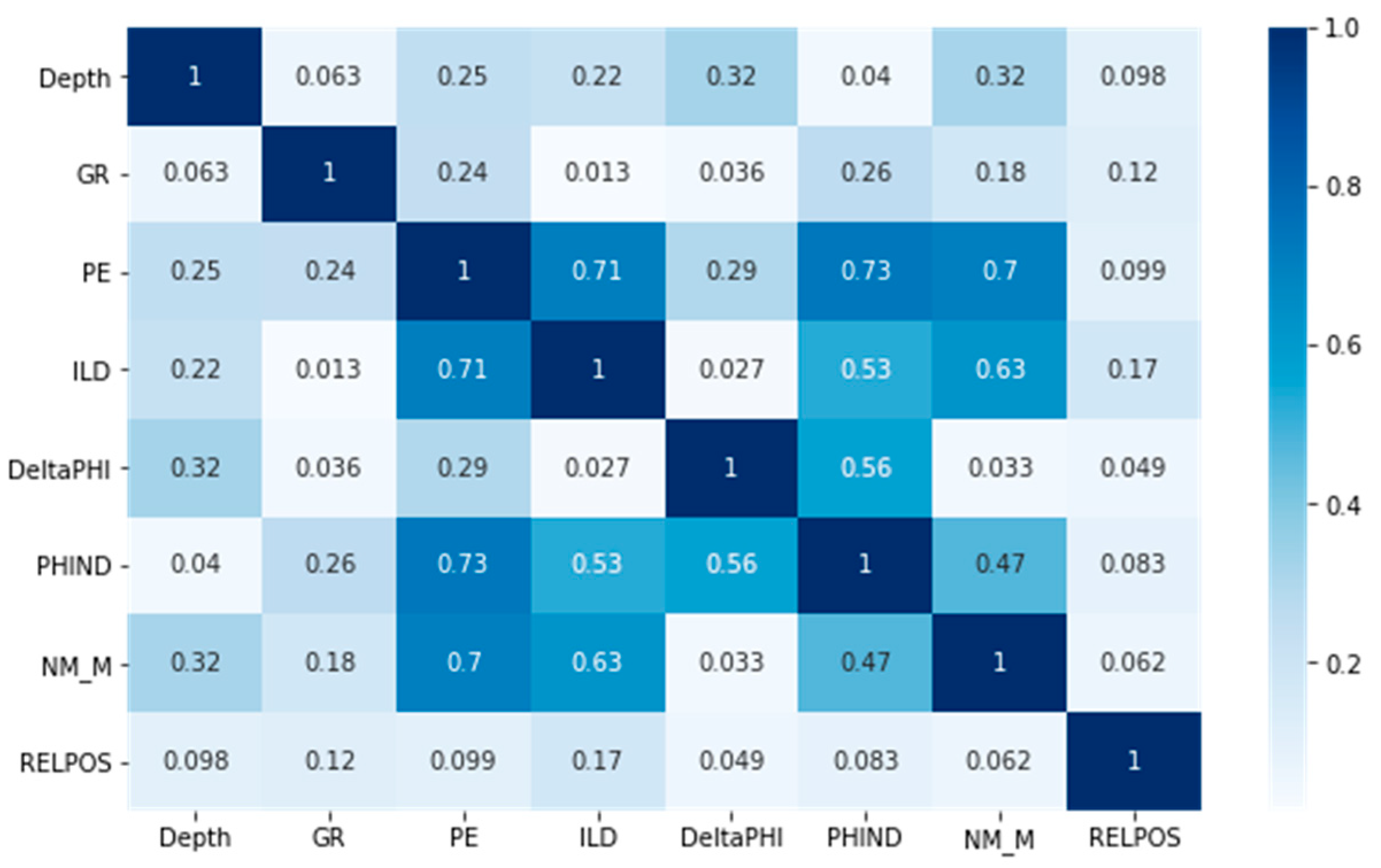
A heat map is often used in practice to display the correlation coefficient matrix of a set of variables [33]. This also has great applicability in displaying the data distribution of the contingency table. Through heat mapping, we can intuitively feel the difference in value size. Figure 5 is a heat map of the above seven logging attributes, as well as depth. The right side of Figure 5 is the color bar, which represents the mapping from value to color. A value from small to large corresponds to the color from light to dark. From the heat map in Figure 5, we can see that the correlation of the photoelectric effect curve (PE) is the best, with the correlation between photoelectric effect (PE) and average of neutron and density logs (PNHIND) being 0.73, the correlation between photoelectric effect (PE) and resistivity (ILD) being 0.71, and the correlation between photoelectric effect (PE) and nonmarine–marine indicator (NM_M) being 0.7. The photoelectric effect is usually included in modern well logs to provide essential information on formation lithology. However, many legacy wells might not have photoelectric effect logs. Therefore, the photoelectric effect was selected as the target curve in this study, and the remaining six attributes were used as the known characteristic values.
Data preprocessing, including data cleaning and normalization, is important to improving the accuracy of data prediction. Professional engineers perform data cleaning to improve the quality of well-logging data by discarding outliers and noisy information using mean substitution and scatterplot visualization methods [34]. Normalization usually refers to the scaling of features to (0,1), a special case of normalization adjustment that has the effects of speeding up training and preventing gradient explosion [35]. In these experiments, to normalize the data, the maximum–minimum scaling adjustment can be simply applied to each feature column, where the new value of the sample can be calculated as follows:
X n o r m = X X m i n X m a x X m i n
where X n o r m is the normalized value of the well-logging curve at the well depth, X m a x is the maximum value, and X m i n is the minimum value. This method is suitable for cases wherein the approximate upper and lower bounds of the data are known, the data have few or no outliers, and the data have an approximately uniform distribution.
After data preprocessing, a data set with a total number of 3232 samples was established in this study. The key characteristics of the well-logging samples are shown in Table 1. In the study, the data were randomly partitioned into an 80:20 split for training and validation data sets, respectively. The first 80% was used as the training set to train the network model, and the second 20% was used as the test set to verify the prediction accuracy of the proposed model.
A model comparison was performed among a suite of machine learning techniques—SVR, GBDT, CNN, LSTM—and the CNN-LSTM hybrid model to validate the effectiveness of the CNN-LSTM model according to the evaluation metrics of the test set. The various models were optimized by the PSO algorithm for comparison.

4.2. Photoelectric Effect Prediction from Other Logs for the Target Well

The first well, denoted as Well 1, in the data set was selected as the target well in this section to verify the prediction accuracy of the hybrid network model for single-well analysis. 
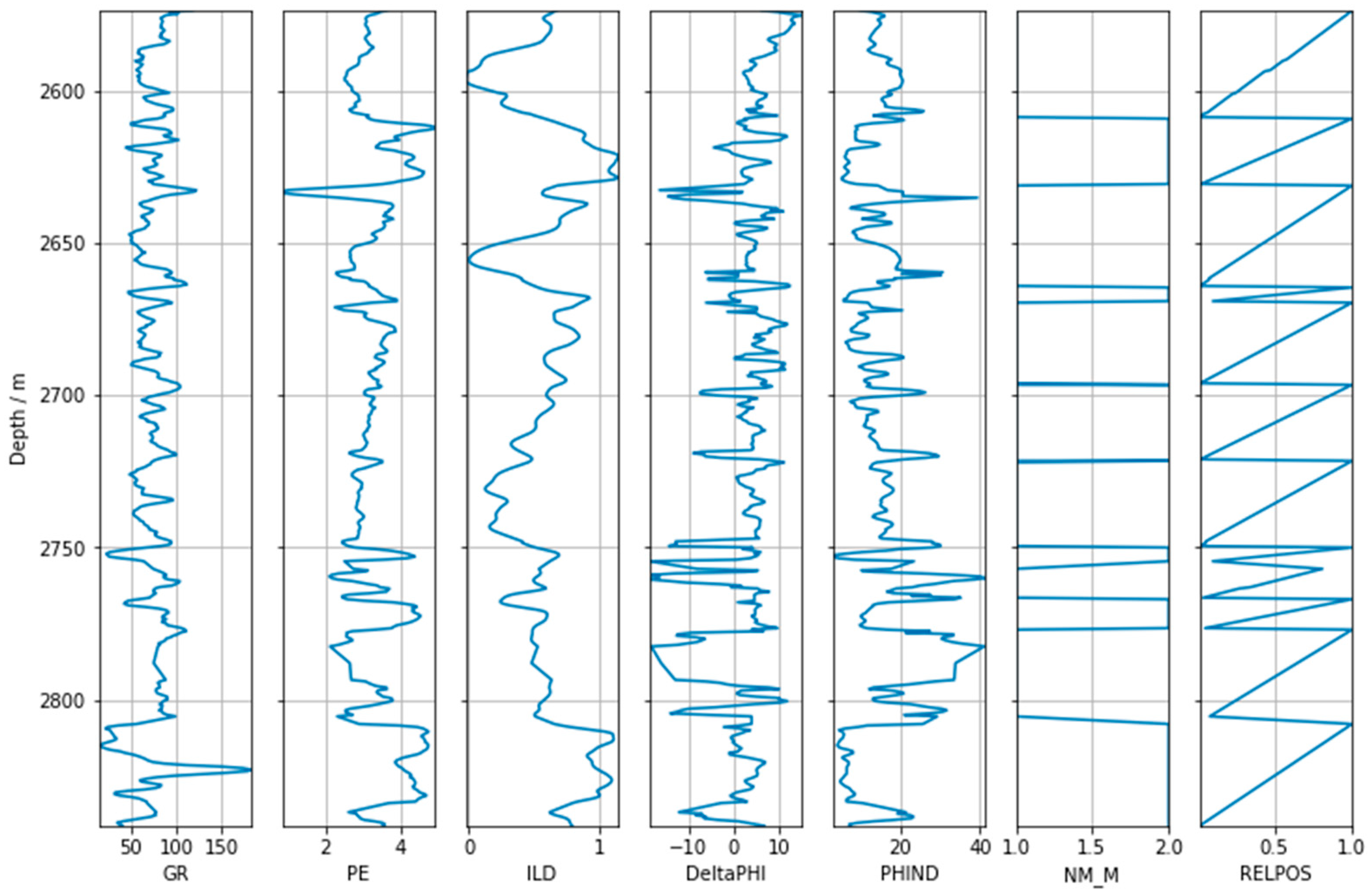
Figure 6 shows the seven well-logging curves of Well 1. In the experiment, Well 1 had six eigenvalues for training and prediction logs: gamma ray (GR), resistivity (ILD), neutron density–porosity difference (DeltaPHI), average of neutron and density logs (PHIND), nonmarine–marine indicator (NM_M), and relative position (RELPOS), and the data set was divided into training and validation sets with a ratio of 80:20. The hybrid CNN-LSTM network model was optimized using the PSO algorithm for predicting the photoelectric effect curve in the validation set. The depth of Well 1 was from 2573.5 to 2841.5 m; therefore, there were 501 sets of data in the well section with a total length of 268 m. The photoelectric effect curves in the last 100 sets of data were manually removed as the prediction targets.

4.2.1. Performance Evaluation of CNN-LSTM-PSO Model

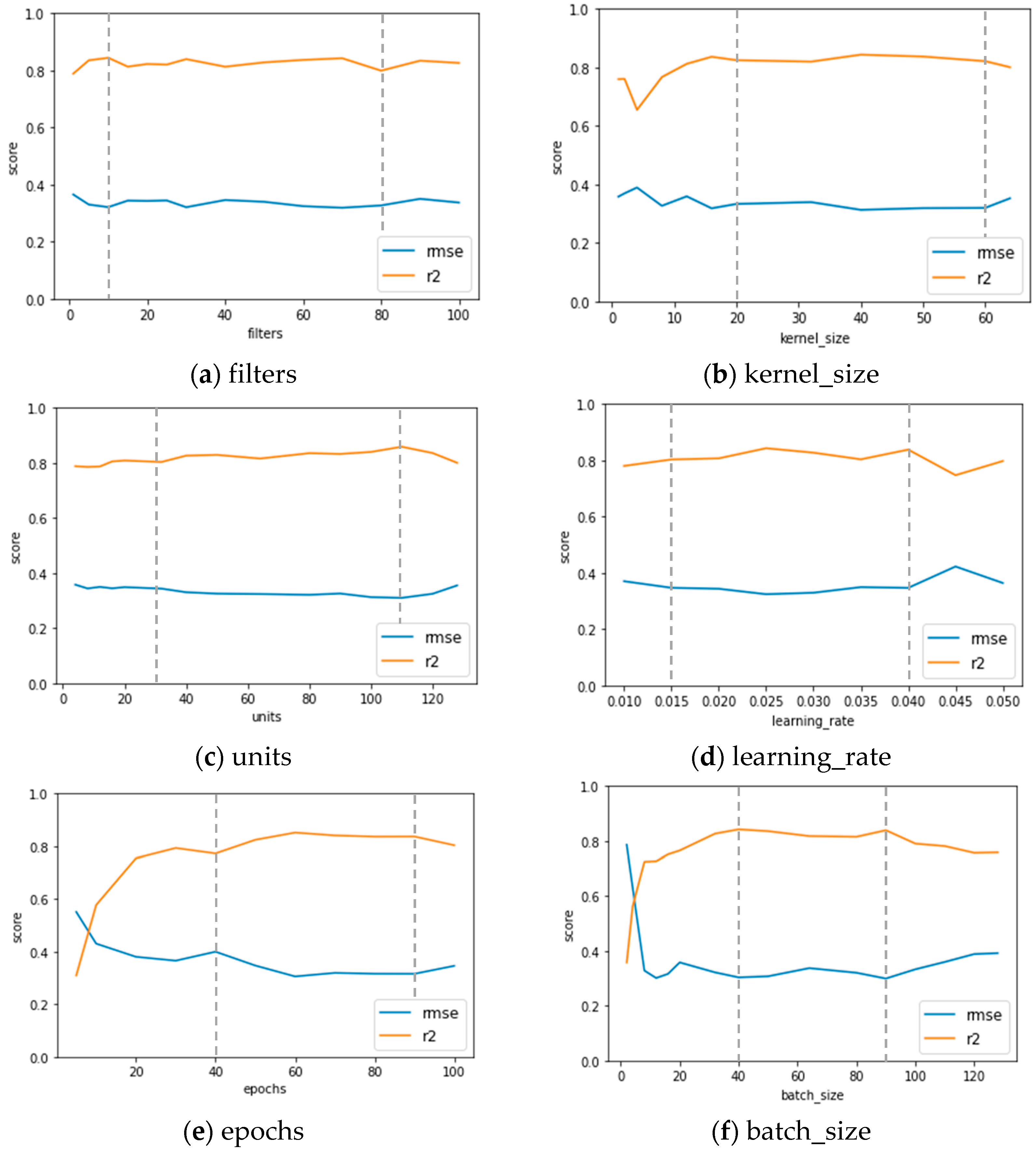
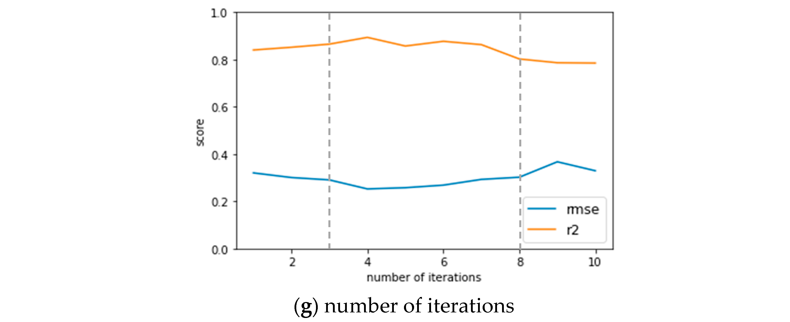
There are seven main hyperparameters in the CNN-LSTM hybrid network model, including filters (the number of CNN filters), kernel_size (the size of the CNN convolutional kernel), units (the number of LSTM hidden neurons), learning_rate (the learning rate of the neural network), epochs (the number of samples trained), batch_size (the size of each batch of data), and number of iterations (the number of times the training data are trained using the network model), which need to be calibrated and determined during PSO iterations. The first step is to analyze the impact of each hyperparameter on the prediction accuracy, and then the analysis result is used to determine the reasonable range of hyperparameters for performing the PSO.
The initial values and ranges of the seven hyperparameters are listed in Table 2. Figure 7 shows the curves of the estimated RMSE and R2 values of each hyperparameter with single-factor analysis by changing one parameter at a time. These curves indicate the effects of each hyperparameter on the prediction accuracy of the logging data. Epochs and batch_size had the greatest effect on the accuracy, as both the RMSE and R2 curves of these two hyperparameters changed with significant variation during PSO iterations. Based on the results shown in Figure 7, reasonable ranges for each hyperparameter for performing further PSO were determined, and are given in Table 2. Furthermore, the CNN-LSTM model with the lowest RMSE and highest R2 among all the CNN-LSTM models in the single-factor analysis was recorded and saved as a reference model before PSO for further comparison. The lowest RMSE was 0.252, and the highest R2 was 0.885 among all the models.
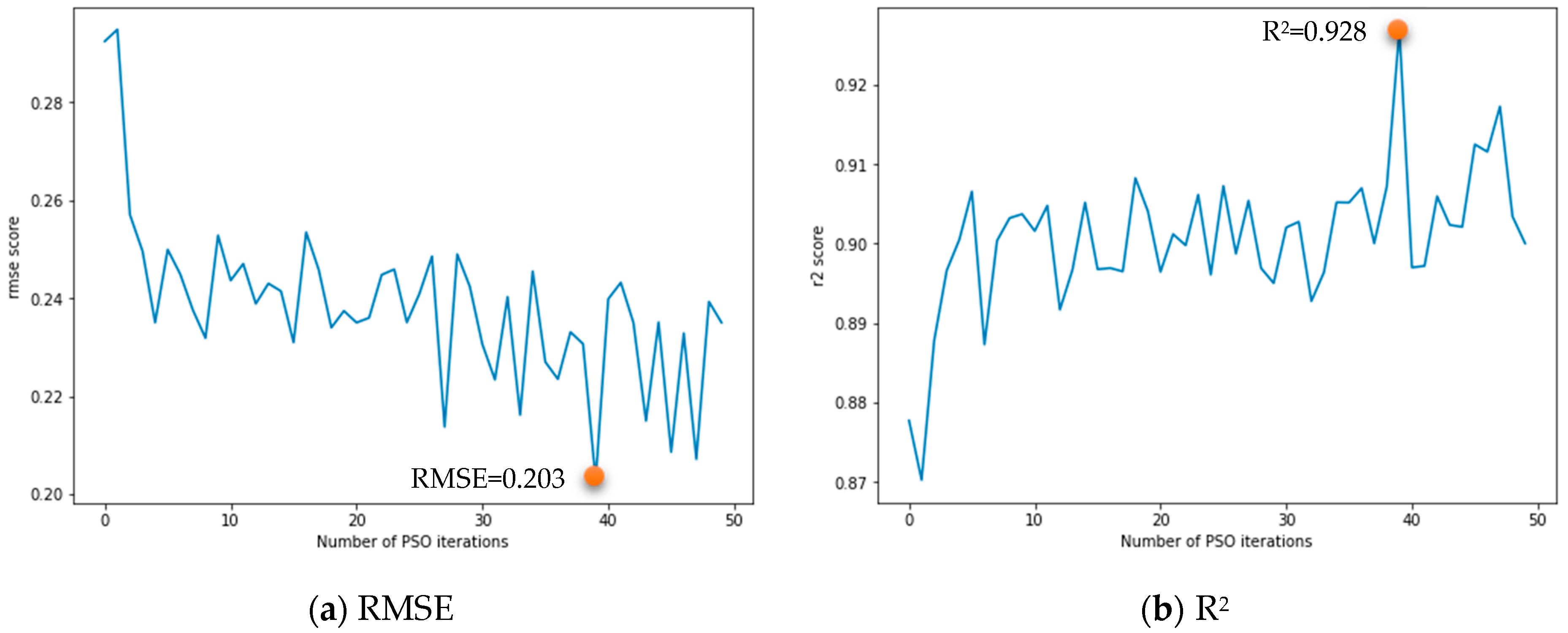
The seven hyperparameters of the CNN-LSTM hybrid network model were selected as the tuning parameters of PSO, and the range of each hyperparameter was finalized according to the results of single-factor analysis. The PSO had a total of 50 iterations with 15 particles each. Figure 8 shows the distribution of the optimal RMSE and R2 for each PSO iteration. As the number of iterations increased, the optimal RMSE showed a decreasing trend and the optimal R2 showed an increasing trend, indicating that the training effect of the proposed model was getting better and tended towards the global optimum value. The hyperparameters of the optimal CNN-LSTM model with the best evaluation metrics after PSO were then obtained and are listed in Table 2. The RMSE of the optimal CNN-LSTM model was 0.203, which is 19% lower than that before the performance of PSO (RMSE = 0.252), and the R2 was 0.928, which is 4.9% higher than that before the performance of PSO (R2 = 0.885). This means that the optimal CNN-LSTM hybrid network model constructed with the seven hyperparameters determined by the PSO algorithm can greatly improve the accuracy of the CNN-LSTM model.
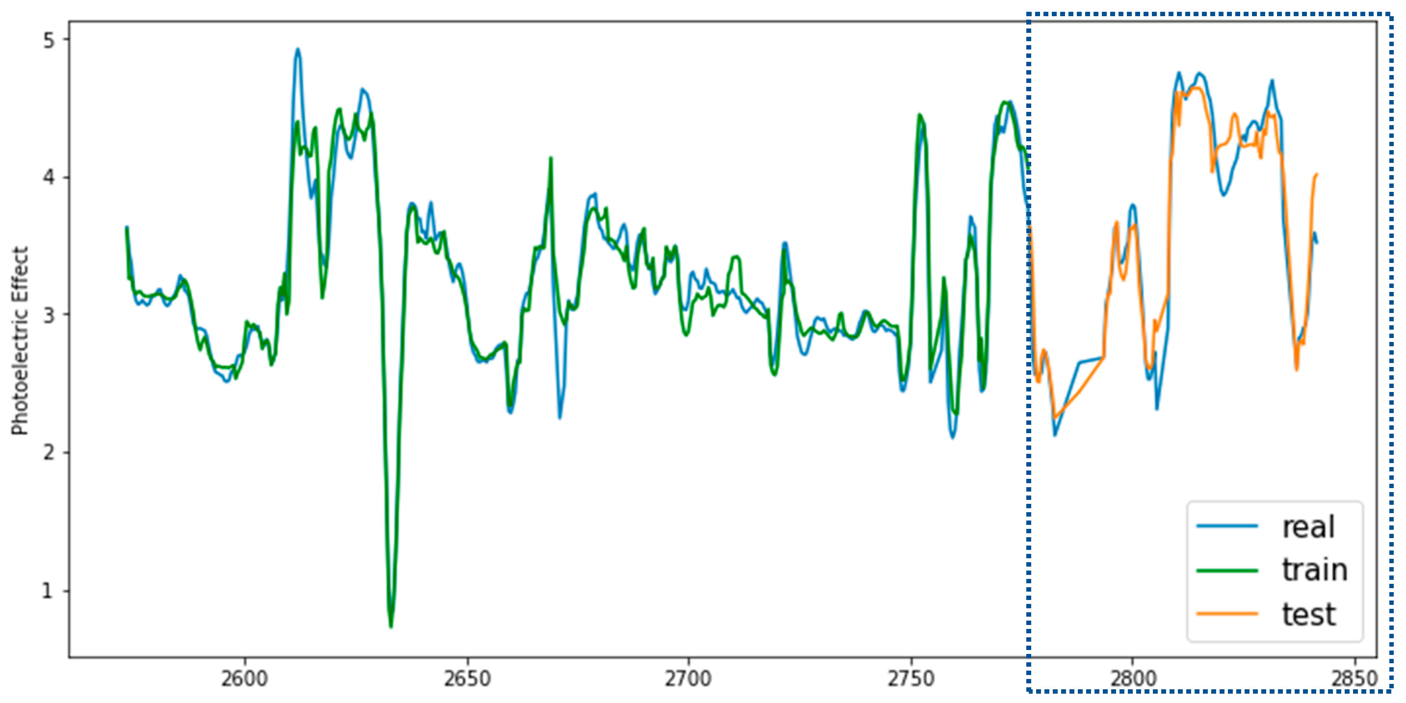
The model with the best prediction was saved through several iterations of the CNN-LSTM-PSO model, and the saved model was used to make predictions for the single-well test data. Figure 9 shows the photoelectric effect curve-matching result for Well 1, where the true value is shown in blue, the predicted photoelectric effect curve of the training data set is shown in green, and the predicted photoelectric effect curve of the test data set is shown in orange. The result shows that the predicted photoelectric effect curves, on both the training and test sets, agreed well with the field logging data.

4.2.2. Model Competition

The CNN-LSTM-PSO model was then compared with traditional machine learning models and deep learning-based AI models for single-well logging prediction analysis. There are many classical machine learning models available for logging curve prediction [36], such as SVR, GBDT, and artificial neural network (ANN). Among these methods, ANN has become a popular method for logging curve prediction, and SVR and GBDT are very effective methods for logging curve prediction as well. These classical algorithms were used in the experiments to generate logging curves, and the PSO algorithm was used to optimize the model hyperparameters for comparison.
Taking the prediction of the photoelectric effect curve as an example, each model was experimented with several times in independent environments to save the optimal model for prediction. First, we looked at the prediction results of the CNN, LSTM, and CNN-LSTM hybrid neural network models, and compared the prediction results of the models by optimizing the hyperparameters of each of the three neural network models with the PSO algorithm. 
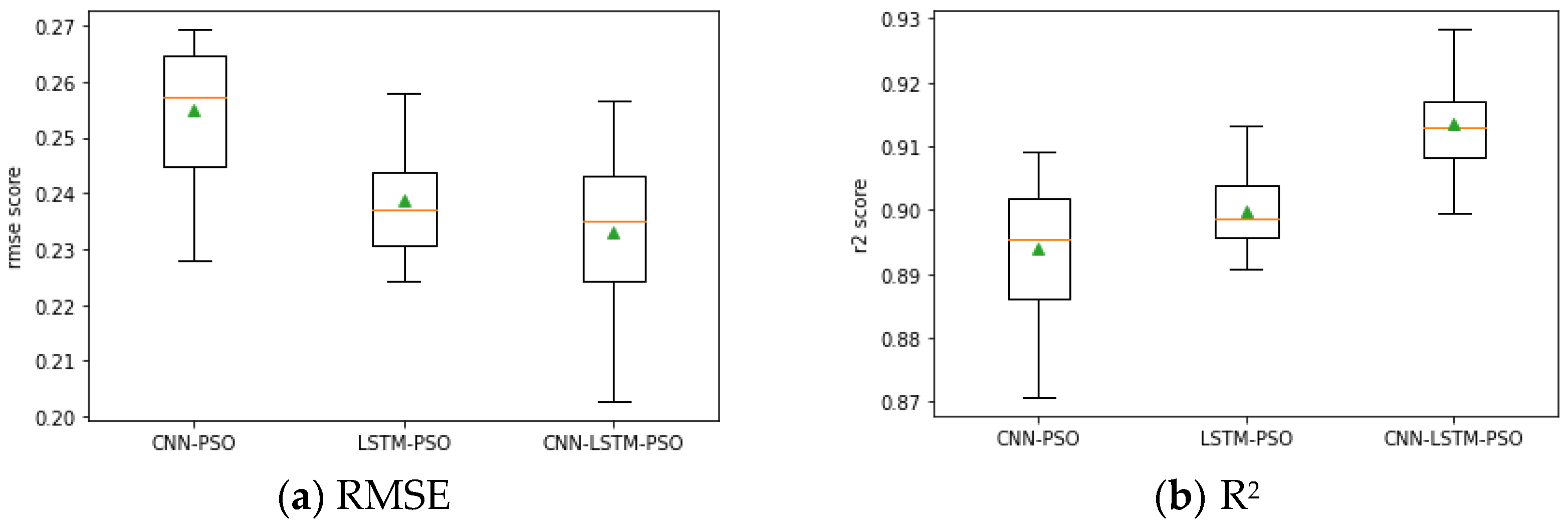
Figure 10 shows a comparison of the best results of the three different neural network models after 10 iterations of the PSO algorithm, with the best value of the lower whisker for RMSE and the best value of the upper whisker for R2. The orange line represents the median value, and the green triangle is the mean value. Figure 10a shows the CNN model as having the worst accuracy, because it has the highest mean RMSE and median RMSE among the three models. The LSTM model and the CNN-LSTM hybrid model are shown to have closer median and mean values. Figure 10b shows the median and mean R2 values of the CNN model to be slightly lower than those of the LSTM model. The median and mean R2 values of the CNN-LSTM hybrid model are better than those of the CNN and LSTM models. Therefore, the hybrid CNN-LSTM neural network model is superior to the CNN and LSTM neural network models alone in terms of prediction accuracy.
Looking at the traditional machine learning models, we chose SVR and GBDT in the scikit-learn library and used the default parameters for both. Table 3 shows the scores of the two evaluation metrics, RMSE and R2, of the photoelectric effect predictions evaluated by the SVR, GBDT, CNN-PSO (optimized CNN network using PSO), LSTM-PSO (optimized LSTM network using PSO), and CNN-LSTM-PSO (hybrid CNN-LSTM network using PSO) models. Among the classical machine learning algorithms, the GBDT model had an RMSE of 0.321 and an R2 of 0.783, which values are better than the SVR model. The CNN-PSO model and the LSTM-PSO model had RMSE values of 0.228 and 0.225 and R2 values of 0.909 and 0.913, which outperform the traditional machine learning methods. The RMSE of the CNN-LSTM-PSO model proposed in this study was 0.203, and its R2 was 0.928—showing the best performance among all the models. The reason may be that the hybrid structures of the CNN, LSTM, and PSO algorithms can fully extract the spatial and temporal features of the well-logging data.
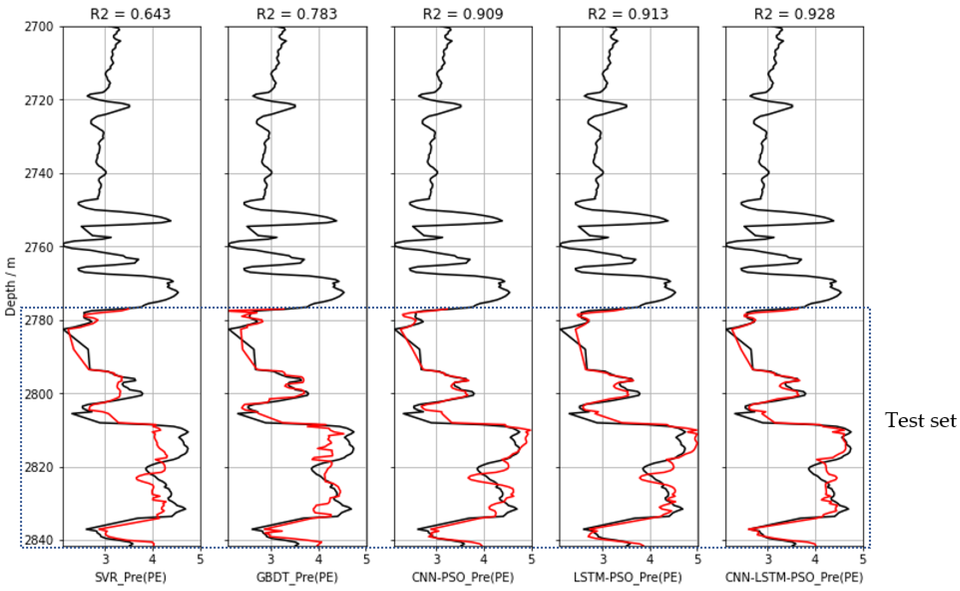
Figure 11 shows the photoelectric effect curves predicted by the SVR, GBDT, CNN-PSO, LSTM-PSO, and CNN-LSTM-PSO models from other logs of Well 1 test data, where black is the actual measured photoelectric effect curve in the oilfield and red is the prediction result on the 20% test set. Overall, there was a good overlay between the measured photoelectric effect and the predicted photoelectric effect for all five models. The R2 values of all models ranged from 0.643 to 0.928, indicating that deep learning can accurately predict the trend of the target photoelectric effect curve. However, combining CNN, LSTM, and PSO algorithms was chosen as the best model, as the logging prediction accuracy is significantly improved in this arrangement, and it is more suitable for predicting the photoelectric effect curve. Therefore, the CNN-LSTM-PSO model was proven to be useful for predicting logging curve sequences from other well logs of the target well itself.

4.3. Photoelectric Effect Prediction from Adjacent Well Logs

This section uses the data of multiple adjacent wells to predict the entire missing curve of the target well. Well 1 was selected as the verification set from the eight wells, so all photoelectric effect curve data of Well 1 were deleted from the data set. In other words, only the logging data of the remaining seven wells, as well as the remaining logging data (expect photoelectric effect data) of Well 1, were used as the training set. In the experiments, a total of six logging feature values was used to train and predict photoelectric effect curves, and the PSO algorithm was used to improve the prediction accuracy of the model. There were 3232 total sets of data derived from all eight wells. Among them, 501 sets of photoelectric effect data of Well 1 were manually removed and treated as the prediction target, and the rest of the data sets from Well 1 and the remaining seven wells were used as the training set.

4.3.1. Performance Evaluation of CNN-LSTM-PSO Model

Table 4 gives the initial ranges of the seven hyperparameters (filter, kernel size, units, learning rate, epoch, batch size, and number of iterations) of the CNN-LSTM hybrid network model as the tuning parameters of the PSO.
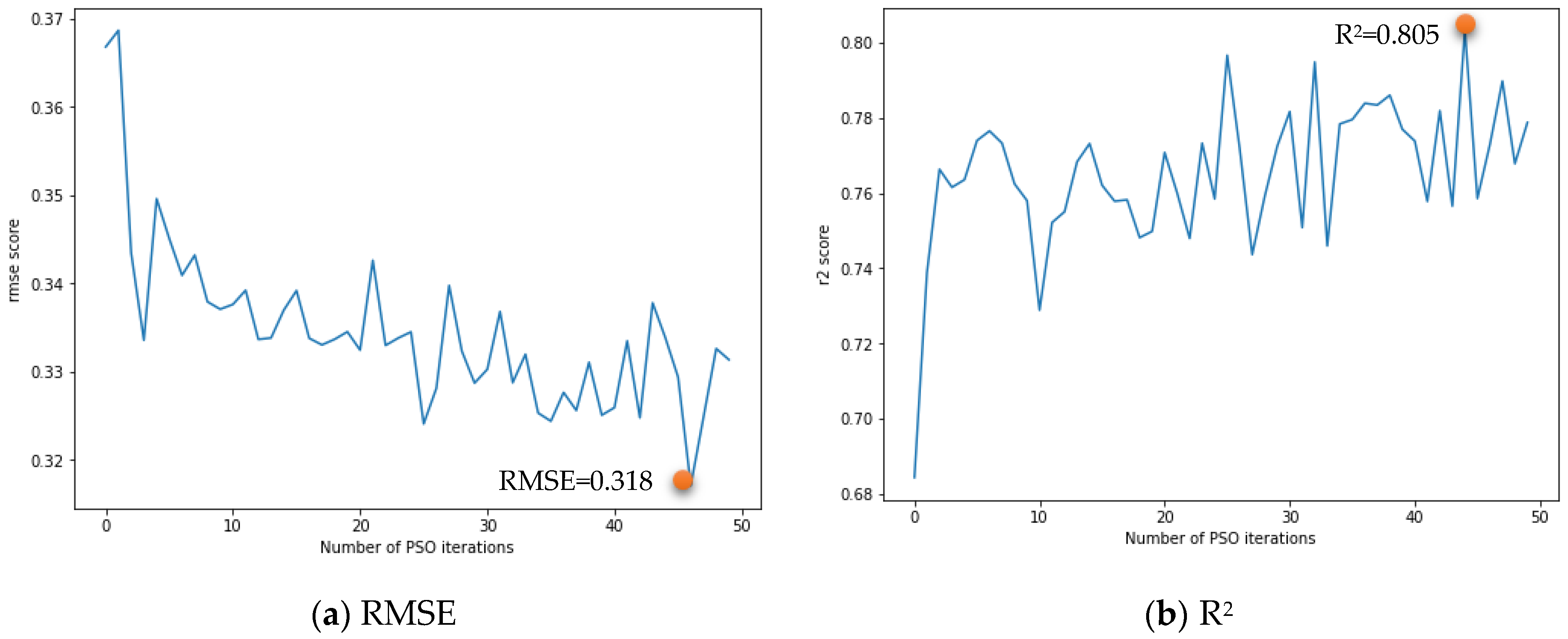
Figure 12 shows the distribution of the optimal values of RMSE and R2 for 50 iterations of PSO, with the optimal values of RMSE and R2 converging towards the global optimal values as the numbers of iterations increased. Based on both the RMSE and R2 values of all PSO iterations, the seven hyperparameters that established the optimal CNN-LSTM model with the lowest RMSE and highest R2 after PSO were determined and are shown in Table 4. The RMSE of the optimal CNN-LSTM model was 0.318, which is 13.1% lower than that before PSO (RMSE = 0.366), and the R2 of the optimal CNN-LSTM model was 0.805, which is 10.3% higher than that before PSO (R2 = 0.73). The result indicates that the CNN-LSTM-PSO hybrid network model used to predict photoelectric effect logs from multiple adjacent wells can also greatly improve the prediction accuracy of missing logging segments.
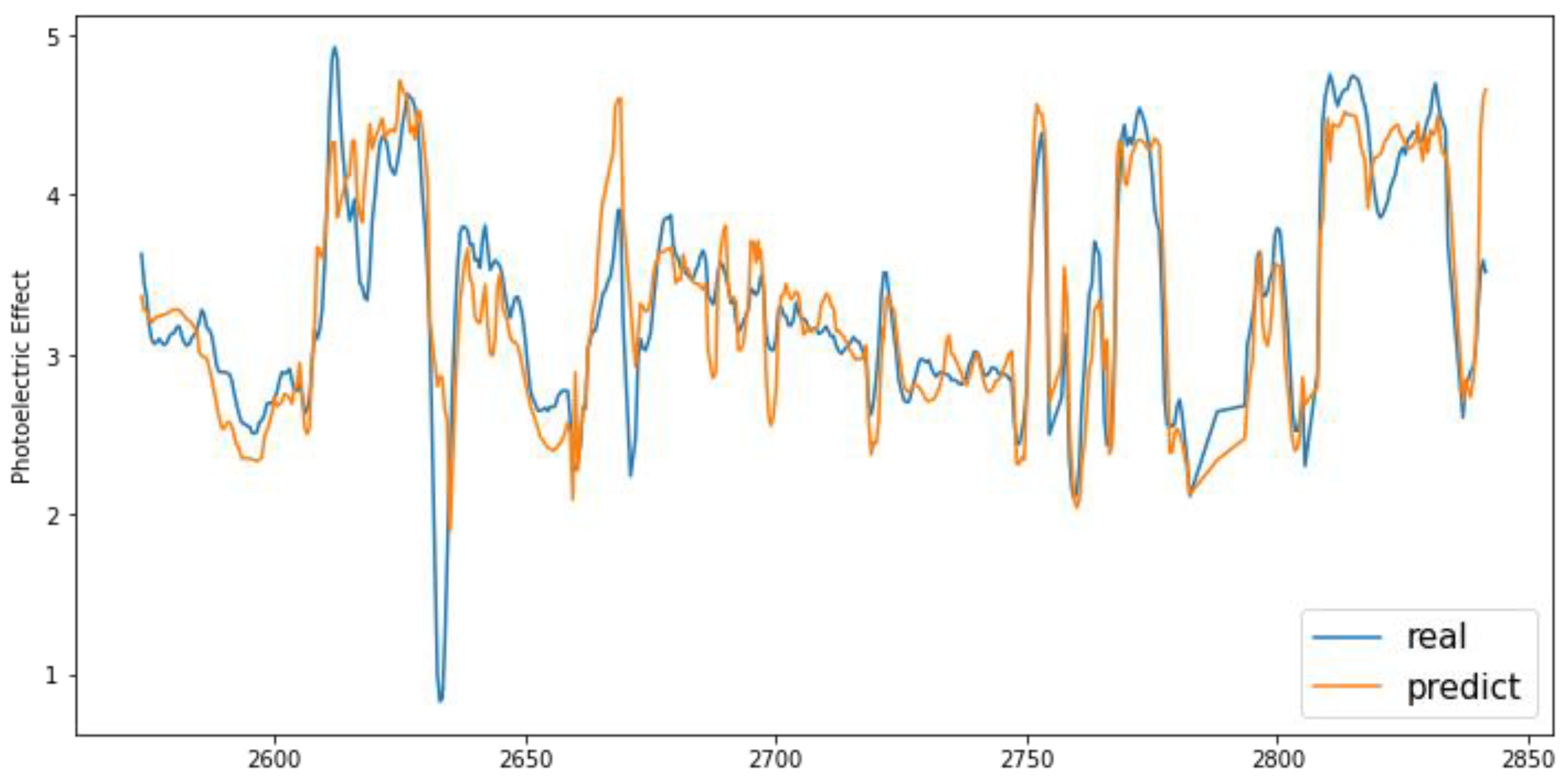
The prediction performance of the CNN-LSTM model optimized by the PSO algorithm was then verified by predicting the photoelectric effect curve of Well 1 on test data sets. Figure 13 shows both the actual measured photoelectric effect curve of Well 1 and the photoelectric effect curve of Well 1 predicted by the CNN-LSTM-PSO model with logs from adjacent wells. The blue curve is the test photoelectric effect data of Well 1, and the orange curve is the photoelectric effect curves of Well 1 estimated by the CNN-LSTM-PSO model with adjacent well information. It is obvious that the photoelectric effect curve predicted by the CNN-LSTM-PSO hybrid network model agrees well with the measured photoelectric effect curve from the test data.

4.3.2. Model Competition

The prediction results of the CNN-LSTM model were compared with those of conventional machine learning models, including SVR, GBDT, CNN, and LSTM. Different models were used in the experiments to generate photoelectric effect curves; SVR and GBDT models used default parameters, and the PSO algorithm was used to optimize the hyperparameters of the CNN, LSTM, and CNN-LSTM models. As an example, for photoelectric effect curve prediction for multiple adjacent wells, each model was run several times in independent environments, and the best prediction model was saved for comparison.
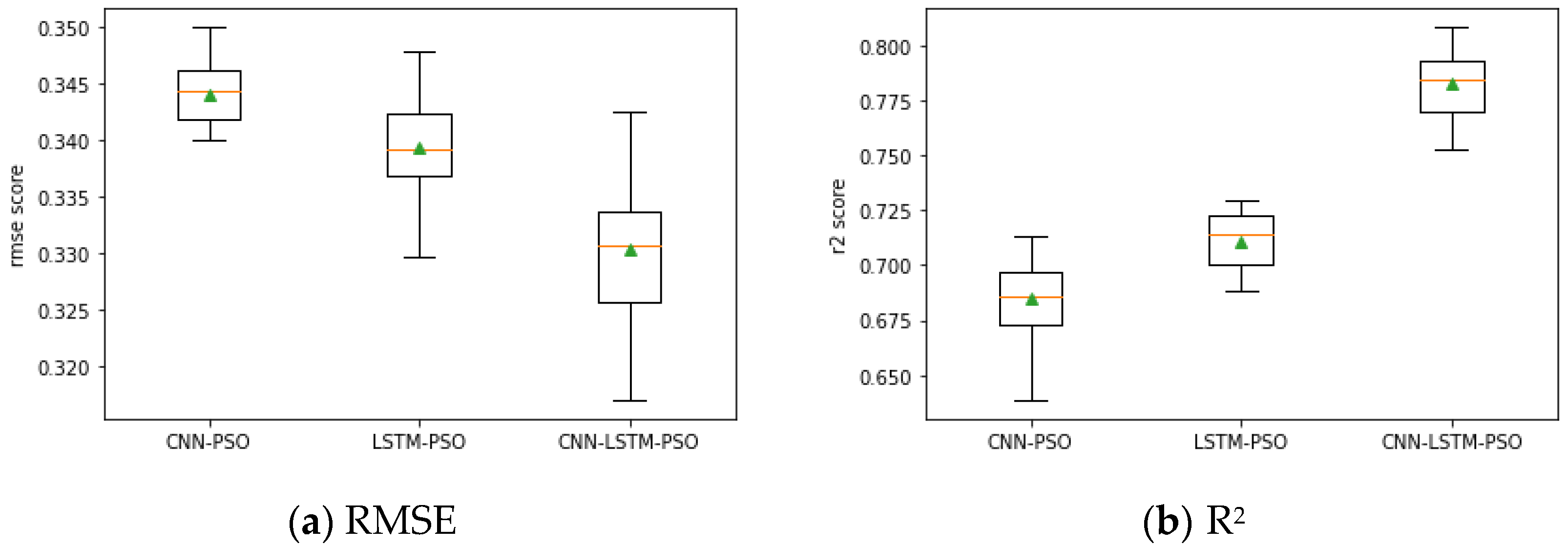
The hyperparameters of the CNN, LSTM, and CNN-LSTM models were optimized by the PSO algorithm, and then the performances of the three models in predicting the whole photoelectric effect curve of Well 1 were examined and compared. Figure 14 shows a comparison of the local optimum scores in the last 10 iterations of the three different neural network models optimized by the PSO algorithm. Analysis of the RMSE and R2 values showed the best and average scores of the CNN-LSTM hybrid neural network model to be better than those of the individual CNN and LSTM neural network models.
The traditional machine learning models SVR and GBDT, with the default parameters in the scikit-learn library, were also investigated and compared with the proposed model. To select the best model, the RMSE and R2 values of the validation data set of the completed models were compared, and the one with the lowest RMSE and highest R2 was selected. 
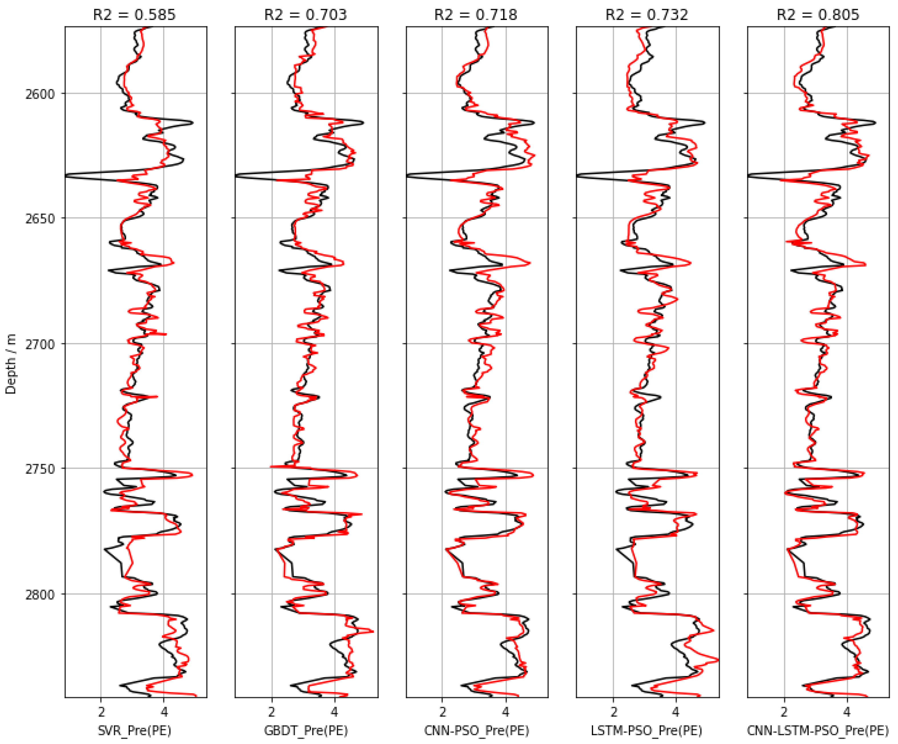
Table 5 shows the scores of the two evaluation metrics used for the photoelectric effect logs predicting by the SVR, GBDT, CNN-PSO, LSTM-PSO, and CNN-LSTM-PSO models with adjacent well information. Among the traditional machine learning algorithms, the GBDT model had an RMSE of 0.359 and an R2 of 0.703, which are significantly better than the SVR model. The CNN-PSO model and the LSTM-PSO model had RMSE values of 0.340 and 0.331, and R2 values of 0.718 and 0.732, which thus outperform the traditional machine learning methods. The RMSE of the CNN-LSTM-PSO model was 0.318, and its R2 was 0.805. The CNN-LSTM-PSO model was obviously the most accurate among all five models.
Figure 15 shows the photoelectric effect curves of Well 1 predicted from multiple adjacent wells by the SVR, GBDT, CNN-PSO, LSTM-PSO, and CNN-LSTM-PSO models. In the figure, black is the actual measured photoelectric effect curve of Well 1 in the oilfield, and red is the prediction result of Well 1. Compared with the actual measured photoelectric effect data, the prediction results of each model had a high degree of fit, indicating that deep learning can accurately predict the trend of the target photoelectric effect curve (Well 1) using the adjacent well information. Combining the CNN, LSTM, and PSO algorithms improves the accuracy of logging prediction, and is more suitable for predicting the target logging curve (Table 5). Therefore, the CNN-LSTM-PSO model also works well in predicting well-logging curve sequences from multiple adjacent wells, but the accuracy is not good enough for comparing with those derived from the other logging data of the target well itself, probably because the correlation between well-logging data from different adjacent wells is not as good as the correlation with the logging data from the well itself. The R2 value of 0.805 in the test data suggests that there is space to improve the architecture. More experiments with the network might yield better results. The study proved that for a newly drilled well, the trained CNN-LSTM-PSO model can also generate a logging curve with the well-logging data of neighboring wells surrounding the new well, but the accuracy needs to be further improved by accounting for geological complexity.

5. Discussion and Future Work

It should be noted that there are still three main problems with AI in well-logging curve prediction applications: (1) the limited number of samples does not accurately and comprehensively reflect the actual geological conditions; (2) the discussion focuses on the AI level, often ignoring the preprocessing of well-logging data, such as missing value processing, outlier correction, and standardization; and (3) there is poor robustness, which does not permit learning methods such as deep reinforcement and adaptive neural network tuning. It does not allow the machine to gradually improve its analysis and adaptation capabilities in the process of building the database. Researchers should take into account the economic applicability and scalability as much as possible while designing the implementation method.
A limitation of the proposed hybrid model was that the accuracy of the logs predicted using the logging data of adjacent wells was not high enough. In the future, we will investigate the inability of the prediction model to efficiently generate missing well-logging curves for any region of interest by considering geological complexity. In order to better conduct this work, it is necessary to deeply integrate neural networks with specific application scenarios [37]. It is not simple to apply machine learning algorithms directly to the logging curve problem, but a more organic and in-depth combination needs to be considered. On the one hand, domain knowledge can be introduced into the machine-learning model by adding physical constraints, for example. On the other hand, it is also possible to improve machine learning models by borrowing features from algorithms used in engineering. Because there are many problems that are not prominent in the computer domain but that need to be faced in engineering practice (e.g., the problem of small samples due to training data not being easily available), there exist instead some algorithms in the engineering domain that specifically deal with such problems that are not available in machine learning. By applying such algorithms to machine learning, there is potential to improve machine-learning models and make them easier to apply to practical engineering domains.

6. Conclusions

In this study, we analyzed the application of AI in well-logging curve reconstruction, and propose a logging prediction method based on the combination of CNN and LSTM with the PSO algorithm, taking into account the developmental trend of AI technology. A field study was conducted with eight wells from the Cornwall Grove natural gas reservoir, Kansas, USA, and the prediction performances of various models were validated and compared. The reason why the proposed model outperformed other conventional networks is discussed and explained. The main conclusions drawn were the following:
  • The proposed CNN-LSTM hybrid network model has highest prediction accuracy compared with traditional machine learning models (Table 3 and Table 5), such as SVR, GBDT, CNN, and LSTM models, as the spatiotemporal information of the well-logging curve is fully considered by the hybrid model;
  • The PSO algorithm can greatly improve the accuracy of the CNN-LSTM model (Figure 8 and Figure 12) and save time when tuning the hyperparameters and determining the optimal construction of the CNN-LSTM model;
  • This experiment was performed for wells in the same area, and the prediction accuracy of PE logs using the logging data of adjacent wells is not as good as that using the other logging data of the target well itself (Table 3 and Table 5), due to geological uncertainties.

Author Contributions

Conceptualization, Z.D. and W.L.; Methodology, L.W.; Software, L.W.; Formal Analysis, Z.D. and W.L.; Investigation, L.W. and W.L.; Data Curation, L.W., C.J. and B.Q.; Writing—Original Draft Preparation, L.W.; Writing—Review & Editing, Z.D.; Visualization, L.W.; Supervision, W.L. All authors provided critical feedback and collaborated in the paper. All authors have read and agreed to the published version of the manuscript.

Funding

This research received no external funding.

Institutional Review Board Statement

Not applicable.

Informed Consent Statement

Informed consent was obtained from all subjects involved in the study.

Data Availability Statement

Not applicable.

Acknowledgments

We would like to thank the Project “Shale Oil Development Study of Chang7 Panke Field”, Project “Fracturing Design Optimization of Multistage Fractured Horizontal Wells in the Lower Temple Bay Field, Yanchang Oilfield” and Project “Innovation and Practical Skills Development Program of Xi’an Shiyou University (YCS21213169)” for their support and valuable discussion. We also extend gratitude to GitHub for making their data available.

Conflicts of Interest

The authors declare no conflict of interest.

References

  1. Darling, T. Well Logging and Formation Evaluation; Elsevier: Amsterdam, The Netherlands, 2005; p. 326. [Google Scholar]
  2. Ellis, D.V.; Singer, J.M. Well Logging for Earth Scientists; Springer: Berlin/Heidelberg, Germany, 2007. [Google Scholar]
  3. Shier, D.E. Well log normalization: Methods and guidelines. Petrophys. SPWLA J. Form. Eval. Reserv. Descr. 2004, 45, 268–280. [Google Scholar]
  4. Alkinani, H.H.; Al-Hameedi, A.T.T.; Dunn-Norman, S.; Flori, R.E.; Alsaba, M.T.; Amer, A.S. Applications of Artificial Neural Networks in the Petroleum Industry: A Review. In Proceedings of the SPE Middle East Oil and Gas Show and Conference, Manama, Bahrain, 18–21 March 2019. [Google Scholar] [CrossRef]
  5. Zhou, Z.-H. Learnware: On the future of machine learning. Front. Comput. Sci. 2016, 10, 589–590. [Google Scholar] [CrossRef]
  6. Friedman, J.H. The Elements of Statistical Learning: Data Mining, Inference, and Prediction; Springer: Berlin/Heidelberg, Germany, 2017. [Google Scholar]
  7. Li, Q.; Peng, H.; Li, J. A survey on text classification: From shallow to deep learning. arXiv 2020, arXiv:2008.00364. [Google Scholar]
  8. Hinton, G.E.; Salakhutdinov, R.R. Reducing the Dimensionality of Data with Neural Networks. Science 2006, 313, 504–507. [Google Scholar] [CrossRef] [PubMed] [Green Version]
  9. LeCun, Y.; Bengio, Y.; Hinton, G. Deep learning. Nature 2015, 521, 436–444. [Google Scholar] [CrossRef] [PubMed]
  10. Wu, P.Y.; Jain, V.; Kulkarni, M.S. Machine learning-based method for automated well-log processing and interpretation. In Proceedings of the 2018 SEG International Exposition and Annual Meeting, Anaheim, CA, USA, 14–19 October 2018. [Google Scholar]
  11. Korjani, M.; Popa, A.; Grijalva, E. A new approach to reservoir characterization using deep learning neural networks. In Proceedings of the SPE Western Regional Meeting, Anchorage, AK, USA, 23–26 May 2016. [Google Scholar] [CrossRef]
  12. Parapuram, G.K.; Mokhtari, M.; Hmida, J.B. Prediction and Analysis of Geomechanical Properties of the Upper Bakken Shale Using Artificial Intelligence and Data Mining. In Proceedings of the Unconventional Resources Technology Conference (URTEC), Austin, TX, USA, 24–26 July 2017. [Google Scholar] [CrossRef]
  13. Yang, L.; Chen, W.; Zha, B. Prediction and application of reservoir porosity by convolutional neural network. Prog. Geophys. 2019, 34, 1548–1555. [Google Scholar]
  14. Mandic, D.; Chambers, J. Recurrent Neural Networks for Prediction: Learning Algorithms, Architectures and Stability; Wiley: Hoboken, NJ, USA, 2001. [Google Scholar] [CrossRef]
  15. Zhang, D.; Yuntian, C.; Jin, M. Synthetic well logs generation via Recurrent Neural Networks. Pet. Explor. Dev. 2018, 45, 629–639. [Google Scholar] [CrossRef]
  16. Pham, N.; Wu, X.; Naeini, E.Z. Missing well log prediction using convolutional long short-term memory network. Geophysics 2020, 85, 1–55. [Google Scholar] [CrossRef]
  17. LeCun, Y.; Boser, B.; Denker, J.S.; Henderson, D.; Howard, R.E.; Hubbard, W.; Jackel, L.D. Backpropagation Applied to Handwritten Zip Code Recognition. Neural Comput. 1989, 1, 541–551. [Google Scholar] [CrossRef]
  18. Albawi, S.; Mohammed, T.A.; Al-Zawi, S. Understanding of a convolutional neural network. In Proceedings of the 2017 International Conference on Engineering and Technology (ICET), Antalya, Turkey, 21–23 August 2017; IEEE: Piscataway, NJ, USA, 2017; pp. 1–6. [Google Scholar]
  19. Huang, G.; Liu, Z.; Van Der Maaten, L. Densely connected convolutional networks. In Proceedings of the IEEE Conference on Computer Vision and Pattern Recognition, Honolulu, HI, USA, 21–26 July 2017; pp. 4700–4708. [Google Scholar] [CrossRef] [Green Version]
  20. Gu, J.; Wang, Z.; Kuen, J. Recent advances in convolutional neural networks. Pattern Recognit. 2018, 77, 354–377. [Google Scholar] [CrossRef] [Green Version]
  21. Li, Y.; Hao, Z.B.; Lei, H. Survey of convolutional neural network. J. Comput. Appl. 2016, 36, 2508–2515. [Google Scholar] [CrossRef]
  22. Hochreiter, S.; Schmidhuber, J. Long short-term memory. Neural Comput. 1997, 9, 1735–1780. [Google Scholar] [CrossRef] [PubMed]
  23. Graves, A. Long Short-Term Memory Supervised Sequence Labelling with Recurrent Neural Networks; Springer: Berlin, Heidelberg, 2012; pp. 37–45. [Google Scholar]
  24. Sainath, T.N.; Vinyals, O.; Senior, A. Convolutional, long short-term memory, fully connected deep neural networks In Proceedings of the 2015 IEEE international conference on acoustics, speech and signal processing (ICASSP), South Brisbane, QLD, Australia. 19–24 April 1995; pp. 4580–4584. [Google Scholar] [CrossRef]
  25. Kennedy, J.; Eberhart, R. Particle swarm optimization. In Proceedings of the ICNN’95-International Conference on Neural Networks, Perth, WA, Australia, 27 November–1 December 1995; Volume 4, pp. 1942–1948. [Google Scholar] [CrossRef]
  26. Poli, R.; Kennedy, J.; Blackwell, T. Particle swarm optimization. Swarm Intell. 2007, 1, 33–57. [Google Scholar] [CrossRef]
  27. Shi, Y.; Eberhart R, C. Empirical study of particle swarm optimization. In Proceedings of the 1999 Congress on Evolutionary Computation-CEC99 (Cat. No. 99TH8406), Washington, DC, USA, 6–9 July 1999; IEEE: Piscataway, NJ, USA, 1999; Volume 3, pp. 1945–1950. [Google Scholar] [CrossRef]
  28. Shi, Y. Particle swarm optimization: Developments, applications and resources. In Proceedings of the 2001 Congress on Evolutionary Computation (IEEE Cat. No. 01TH8546), Seoul, Korea, 27–30 May 2021; IEEE: Piscataway, NJ, USA, 2001; Volume 1, pp. 81–86. [Google Scholar]
  29. Wang, D.; Tan, D.; Liu, L. Particle swarm optimization algorithm: An overview. Soft Comput. 2017, 22, 387–408. [Google Scholar] [CrossRef]
  30. Kim, J.; Lee, K.; Choe, J. Efficient and robust optimization for well patterns using a PSO algorithm with a CNN-based proxy model. J. Pet. Sci. Eng. 2021, 207, 109088. [Google Scholar] [CrossRef]
  31. Willmott, C.J.; Matsuura, K. Advantages of the mean absolute error (MAE) over the root mean square error (RMSE) in assessing average model performance. Clim. Res. 2005, 30, 79–82. [Google Scholar] [CrossRef]
  32. Zhang, D.A. Coefficient of determination for generalized linear models. Am. Stat. 2017, 71, 310–316. [Google Scholar] [CrossRef]
  33. Metsalu, T.; Vilo, J. ClustVis A web tool for visualizing clustering of multivariate data using Principal Component Analysis and heatmap. Nucleic Acids Res. 2015, 43, W566–W570. [Google Scholar] [CrossRef] [PubMed]
  34. Winkler, W.E. Data cleaning methods. In Proceedings of the ACM SIGKDD Workshop on Data Cleaning, Record Linkage, and Object Consolidation, Washington, DC, USA, 24–27 August 2003. [Google Scholar]
  35. Salimans, T.; Kingma, D.P. Weight normalization: A simple reparameterization to accelerate training of deep neural networks. Adv. Neural Inf. Process. Syst. 2016, 29, 901–909. [Google Scholar]
  36. Mohri, M.; Rostamizadeh, A.; Talwalkar, A. Foundations of Machine Learning; MIT Press: Boston, MA, USA, 2012. [Google Scholar]
  37. Duan, J.; Yang, C.; He, J. A ROP Optimization Approach Based on Well Log Data Analysis Using Deep Learning Network and PSO. In Proceedings of the 2019 IEEE International Conference of Intelligent Applied Systems on Engineering (ICIASE), Fuzhou, China, 26–29 April 2019; IEEE: Piscataway, NJ, USA, 2019; pp. 86–88. [Google Scholar] [CrossRef]
Figure 1. Schematic diagram of one-dimensional convolution.
Energies 14 08583 g001
Figure 2. LSTM network structure (adapted from Sainath et al. [24]).
Energies 14 08583 g002
Figure 3. PSO process.
Energies 14 08583 g003
Figure 4. Workflow of the CNN-LSTM-PSO. GR: gamma ray, ILD: resistivity, RELPOS: relative position.
Energies 14 08583 g004
Figure 5. Heat map related to single-well prediction data set. GR: gamma ray, PE: photoelectric effect, ILD: resistivity, DeltaPHI: neutron density–porosity difference, PHIND: average of neutron and density logs, NM_M: nonmarine–marine indicator, RELPOS: relative position.
Energies 14 08583 g005
Figure 6. Complete well-logging curve of Well 1. GR: gamma ray, PE: photoelectric effect, ILD: resistivity, DeltaPHI: neutron density–porosity difference, PHIND: average of neutron and density logs, NM_M: nonmarine–marine indicator, RELPOS: relative position.
Energies 14 08583 g006
Figure 7. Single-factor analysis of CNN-LSTM hybrid network model.
Energies 14 08583 g007aEnergies 14 08583 g007b
Figure 8. RMSE and R2 of CNN-LSTM model during PSO iterations with the training set.
Energies 14 08583 g008
Figure 9. CNN-LSTM-PSO model performance evaluation. The photoelectric effect curve predicted by the CNN-LSTM-PSO model agreed well with the real logging data on training and test data.
Energies 14 08583 g009
Figure 10. Comparison of the RMSE and R2 of CNN, LSTM, and CNN-LSTM after PSO.
Energies 14 08583 g010
Figure 11. Model performance. Black curves are the original measured photoelectric effect (PE) data of Well 1. Red curves are photoelectric effect (PE) generated by various models using other logs of Well 1 test data. R2 values are given on the top of each panel for comparing the various models.
Energies 14 08583 g011
Figure 12. RMSE and R2 of CNN-LSTM model during PSO iterations applied to the training data set.
Energies 14 08583 g012
Figure 13. Performance of CNN-LSTM-PSO model applied to test data.
Energies 14 08583 g013
Figure 14. Comparison of RMSE and R2 accuracy of CNN, LSTM, and CNN-LSTM.
Energies 14 08583 g014
Figure 15. Model performance. Black curve is the original measured photoelectric effect (PE) data. Red curves are photoelectric effect (PE) generated by various models both on training set and test set with the logging data of adjacent wells. R2 values are given on the top of each panel to compare the various models.
Energies 14 08583 g015
Table 1. Data set of main features of seven well logs.
Depth (m)GR (API)PEILD (Ω·m)DeltaPHIPHINDNM_MRELPOS
Mean2702.36072.6993.3300.5692.97514.8691.2970.506
Std76.64521.0630.6670.2905.8807.2430.4580.289
Min2573.513.8930.833−0.026−18.72.9510.013
25%263760.3062.8770.3541.39.1510.259
50%2700.573.6473.2010.5814.213.810.5
75%2764.585.0683.7150.747618.220.759
Max2841.5184.0214.9251.14715.141.3521
Note. GR: gamma ray, PE: photoelectric effect, ILD: resistivity, DeltaPHI: neutron density–porosity difference, PHIND: average of neutron and density logs, NM_M: nonmarine–marine indicator, RELPOS: relative position.
Table 2. Initial values and ranges of the main hyperparameters.
HyperparametersInitial ValueInitial RangeFinal Range Determined by Single-Factor AnalysisValue of the Optimal CNN-LSTM Model by PSO
Filters50[1,100][10,80]44
Kernel size32[1,64][20,60]41
Units50[1,128][30,110]75
Learning_rate0.02[0.01,0.05][0.15,0.04]0.02
Epochs50[1,100][40,90]59
Batch_size64[1,128][40,90]89
Number of iterations2[1,10][3,8]3
Table 3. Evaluation metrics of various models from the other logs of target well test data.
ModelRMSER2
SVR0.3510.643
GBDT0.3210.783
CNN-PSO0.2280.909
LSTM-PSO0.2250.913
CNN-LSTM-PSO0.2030.928
Table 4. Initial ranges and final values of the main hyperparameters.
HyperparametersInitial RangeValue in the Optimal CNN-LSTM Model
Filters[10,80]19
Kernel size[20,60]38
Units[30,110]38
Learning_rate[0.15,0.04]0.015
Epochs[40,90]69
Batch_size[40,90]88
Number of iterations[3,8]5
Table 5. Comparison of RMSE and R2 for multi-well test data.
ModelRMSER2
SVR0.3940.585
GBDT0.3590.703
CNN-PSO0.3400.718
LSTM-PSO0.3310.732
CNN-LSTM-PSO0.3180.805
Publisher’s Note: MDPI stays neutral with regard to jurisdictional claims in published maps and institutional affiliations.

