Research on Dynamic Modeling of KF Algorithm for Detecting Distorted AC Signal

Abstract

Kalman filter (KF) is often based on two models, which are phase angle vector (PAV) model and orthogonal vector (OV) model, in the application of distorted grid AC signal detection. However, these two models lack rigorous and detailed derivation from the principle of dynamic modeling. This paper presents a phase angle vector dynamic (PAVD) model and an orthogonal vector dynamic (OVD) model, which are combined with Kalman filter for detecting distorted grid AC signal. They reveal that the state noise covariance of the dynamic model−based KF is related to the sampling cycle, and overcome the defect of more detecting error for conventional model−based KF. Experiment and evaluation results show that the proposed KF algorithms are reasonable and effective. Therefore, this paper contributes a guiding significance for the application of KF algorithm in harmonic detection.

1. Introduction

The Kalman filter (KF) plays an increasingly important role in the real−time detection of grid AC signal [1]. It was first applied to the power signal processing field by Dr. A. A. Girgis in 1981 [2,3,4]. It mainly applies to the following fields: fundamental and harmonic components detection of grid voltage/current [5,6,7,8,9,10], phase−locked loop synchronization [11,12,13,14,15], power quality detection and compensation equipment [16,17,18,19,20], power disturbance feature extraction and machine classification [21,22,23,24], and etc. In these applications, two conventional models, phase angle vector (PAV) model and orthogonal vector (OV) model, are mainly used. The phase angles were used as vectors to establish a state-space model which could be called the phase angle vector (PAV) model through cosine expansion [3]. The orthogonal vector was used to establish a state-space model that could be called the orthogonal vector (OV) model [4]. However, the state noise covariance of the two models is only a given value based on empirical statistics of the AC signal. It is selected as a fixed value, such as Q = 0.05 × I (I represents the unit matrix), when AC signal is the grid voltage [10,11]. It is selected as a fixed value, such as Q = 0.01 × I, when the AC signal is the sampling current [20]. It is mainly to avoid big tracking error and enable to detect response without time delay. With the development of computer hardware and sensor technology, the sampling cycle is getting smaller, and the accuracy requirements are getting higher. The detecting accuracy of the fundamental and harmonics components for the conventional detecting model−based KF algorithm cannot meet the requirements of modern engineering applications.

The current issue is that the detecting accuracy of the fundamental and harmonics components for the conventional detecting model–based KF algorithm cannot meet the requirements of modern engineering applications. There is no fixed rule as references to find the fixed value by applying different sampling cycles. As a result, the detection accuracy cannot achieve the expected goal.

Also, the discretization model lacks of theoretical basis. In view of the fact that the previous literature did not detailedly derive the PAV and OV model from the principle of dynamic modeling. This paper proposes a phase angle vector dynamic (PAVD) model−based KF (PAVD−KF) algorithm and the orthogonal vector dynamic (OVD) model−based KF algorithm (OVD−KF) through model derivation according to the stochastic process theory [12]. It reveals that the state noise covariance of the conventional detecting model is related to the sampling cycle.

This paper contributes:

(1)

We derive the discretization model from the continuous differential equation in accordance with stochastic process theory, to find the value law of fixed value of covariance under different sampling cycles.

(2)

We greatly improve the detecting accuracy of fundamental and harmonics components, enabling the detection results to meet the requirements of modern engineering applications of AC current and voltage signal.

Section 1 introduces the Kalman filter mainly applies to the following fields and model−based KF existing problems. In Section 2, the related works about conventional PAV and OV model are introduced. In Section 3, the PAVD and OVD models are rederived according to of stochastic process theory. Then, the PAVD−KF and OVD−KF algorithms are proposed. In Section 4, the performances of PAVD−KF and OVD−KF algorithms are evaluated and compared by the experimental current and voltage sampling data. Section 5 concludes the paper.

2. Related Work

In this section, we proposed the expression of distorted AC signal first, and introduce the conventional PAV−KF and OV−KF algorithms then.

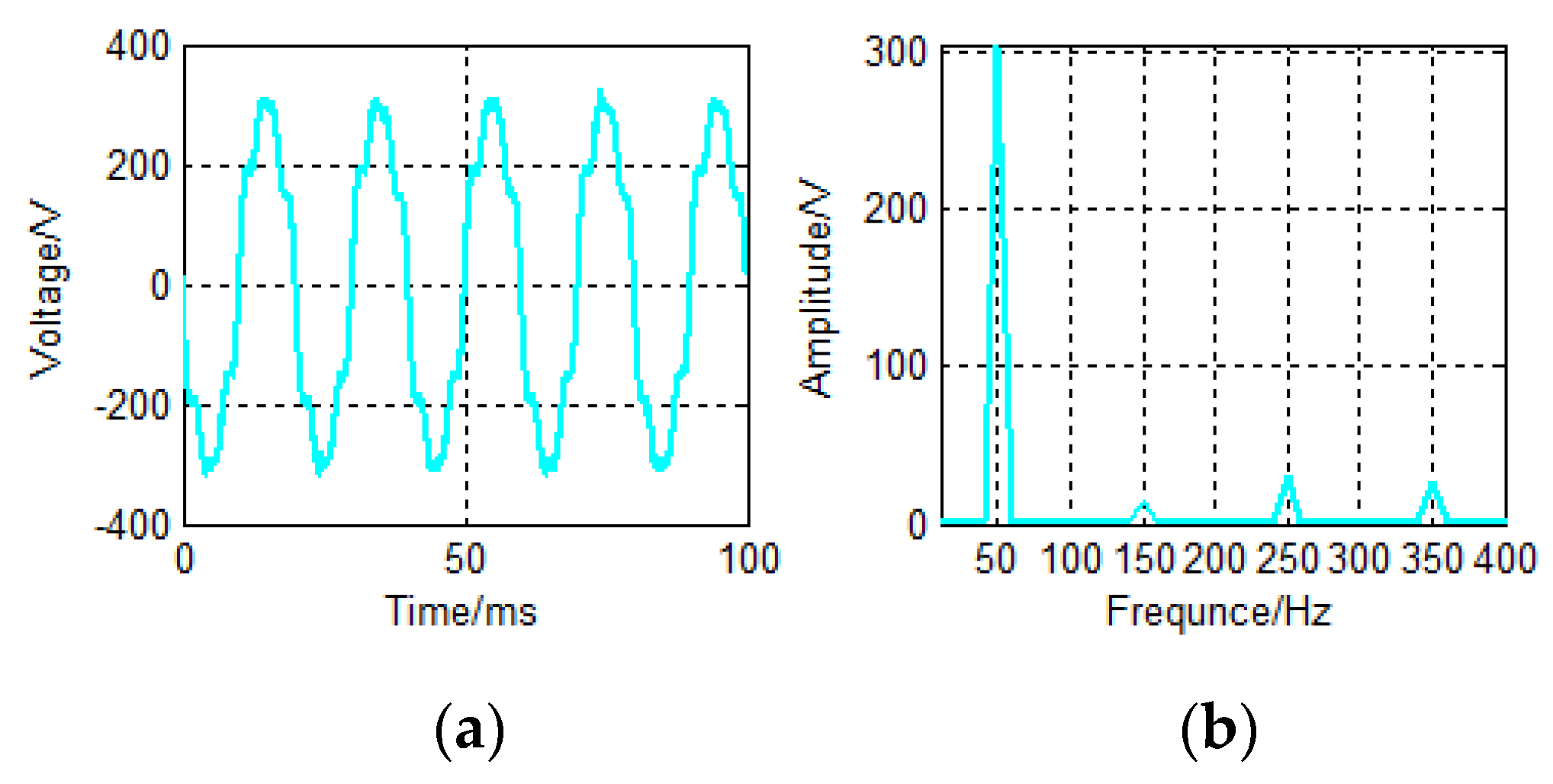
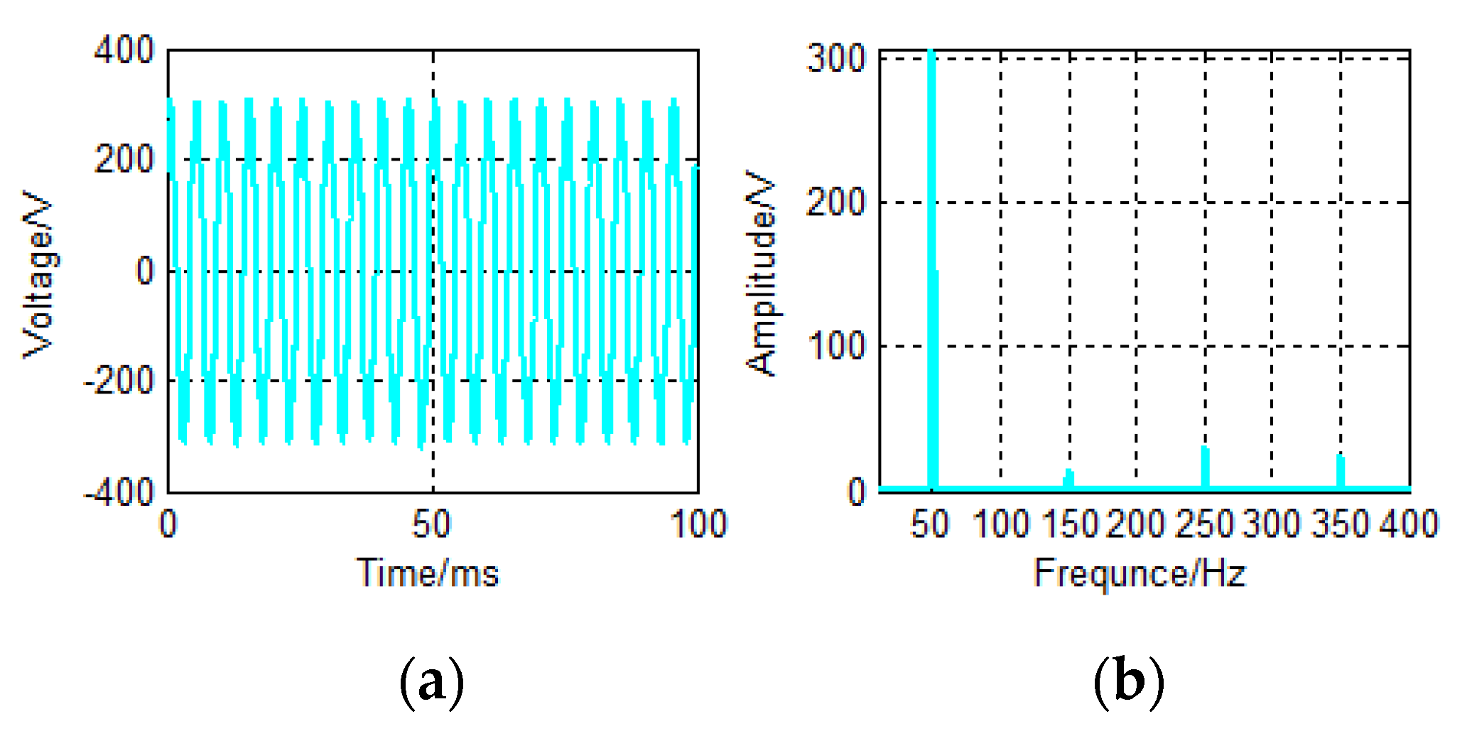
2.1. Distorted AC Signal

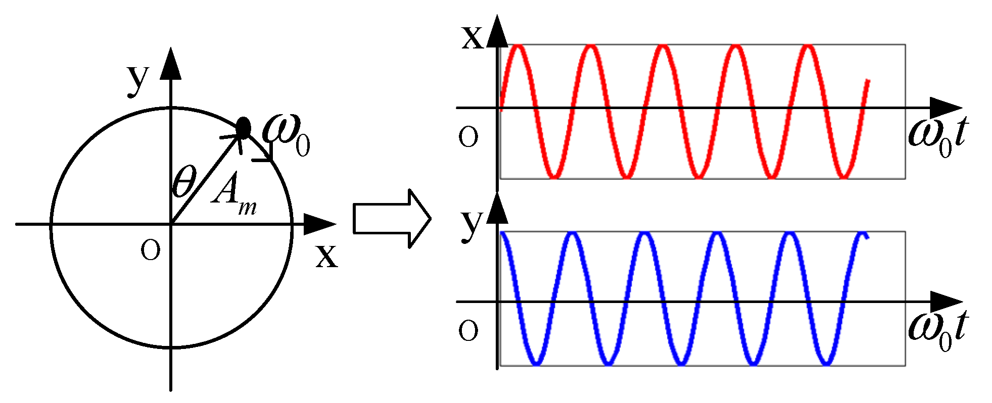
The waveform of the distorted AC signals sampled at time t can be expressed as

$$\mathrm{s}(t)={\displaystyle \sum _{i=1}^N{A}_i(t)\sin [i{\omega }_{0}T+{\theta }_i(t)]+{\displaystyle \sum _{i=1}^N{w}_i(t)}}$$

(1)

where $i=1,2,3,\cdots ,N$, T denotes the sampling cycle. For the fundamental frequency of 50 Hz, ${\omega }_0=100\pi$. ${\displaystyle \sum _{i=1}^N{A}_i(t)\sin [i{\omega }_{0}T+{\theta }_i(t)]}$ represents the fundamental and harmonic components. ${\displaystyle \sum _{i=1}^N{w}_i(t)}$ is the state noise of fundamental and harmonic components.

2.2. PAV Model

The vector of fundamental and harmonic components is expressed as $X_k={\left[\begin{array}{ccccc}{x}_1& y_1& \cdots & x_n& y_n\end{array}\right]}^T$, where $x_1=A_1\cos {\theta }_1$, $y_1=A_1\sin {\theta }_1$,$x_n=A_n\cos {\theta }_n$, $y_n=A_n\sin {\theta }_n$.

The measurement equation of model is expressed as [3]

$$z_k=H_k{X}_k+V_k={\left[\begin{array}{c}\cos ({\omega }_{0}kT)\\ -\sin ({\omega }_{0}kT)\\ ⋮\\ \cos (n{\omega }_{0}kT\\ -\sin (n{\omega }_{0}kT)\end{array}\right]}^T{\left[\begin{array}{c}{x}_1\\ y_1\\ ⋮\\ x_n\\ y_n\end{array}\right]}_k+V_k$$

(2)

The state equation of model is expressed as

$$X_{k+1}={\Phi }_k{X}_k+W_{\mathrm{k}}=\left[\begin{array}{ccccc}1& 0& \cdots & 0& 0\\ 0& 1& \cdots & 0& 0\\ ⋮& ⋮& ⋮& ⋮& ⋮\\ 0& 0& \cdots & 1& 0\\ 0& 0& \cdots & 0& 1\end{array}\right]{\left[\begin{array}{c}{x}_1\\ y_1\\ ⋮\\ x_n\\ y_n\end{array}\right]}_k+{\left[\begin{array}{c}{W}_{x_1}\\ W_{y_1}\\ ⋮\\ W_{x_n}\\ W_{y_n}\end{array}\right]}_k$$

(3)

The covariance matrix of state noise $W_k$ can be expressed as

$$Q_k=E\left[W_k{W}_k^T\right]={\sigma }_{PAV}^2{I}_{2n\times 2n}$$

(4)

2.3. OV Model

Considering a signal $A_k\sin ({\omega }_k{t}_k+{\theta }_k)$ with amplitude $A_k$, angular frequency is ${\omega }_k$ and phase is ${\theta }_k$ [4,11]. Let $x_k=A_k\sin ({\omega }_k{t}_k+{\theta }_k)$, $y_k=A_k\cos ({\omega }_k{t}_k+{\theta }_k)$, initially, consider $A_{k+1/k}\approx A_k$, ${\omega }_{k+1/k}\approx {\omega }_k$ and ${\theta }_{k+1/k}\approx {\theta }_k$. At the time $t_{k+1}=t_k+T$, the signal $x_k$ can be expressed as

$$x_{k+1}=A_{k+1}\sin ({\omega }_k{t}_k+{\omega }_{k}T+{\theta }_k)=x_k\cos ({\omega }_{k}T)+y_k\sin ({\omega }_{k}T)$$

(5)

where, $T$ is the sampling cycle. Additionally,

$$y_{k+1}=A_{k+1}\cos ({\omega }_k{t}_k+{\omega }_{k}T+{\theta }_k)=-x_k\sin ({\omega }_{k}T)+y_k\cos ({\omega }_{k}T)$$

(6)

the state−space is extended for detection of distorted AC signal existed n frequencies harmonic components.

The vectors are expressed as $X_k={\left[\begin{array}{ccccc}{x}_1& y_1& \cdots & x_n& y_n\end{array}\right]}_k^T$, where, $x_{1_k}=A_{1_k}\sin \left({\omega }_k{t}_k+{\theta }_{1_k}\right)$, $y_{1_k}=A_{1_k}\cos \left({\omega }_k{t}_k+{\theta }_{1_k}\right)$, $x_{n_k}=A_{n_k}\sin \left(n{\omega }_k{t}_k+{\theta }_{n_k}\right)$, $y_{n_k}=A_{n_k}\cos \left(n{\omega }_k{t}_k+{\theta }_n{}_{{}_k}\right)$.

Then, the state and measurement equation is expressed as [4]

$$\{\begin{array}{l}{X}_{k+1}=\left[\begin{array}{ccc}{\Phi }_1& \cdots & 0\\ ⋮& \cdots & ⋮\\ 0& \cdots & {\Phi }_n\end{array}\right]X_k+W_{i_k}\\ z_k=\left[\begin{array}{ccccc}1& 0& \cdots & 1& 0\end{array}\right]X_k+V_k\end{array}$$

(7)

where, the state transition matrixes ${\Phi }_i$ are shown below as

$${\Phi }_i=\left[\begin{array}{cc}\cos (i{\omega }_{k}T)& \sin (i{\omega }_{k}T)\\ -\sin (i{\omega }_{k}T)& \cos (i{\omega }_{k}T)\end{array}\right]$$

(8)

The covariance matrix of state noise $W_{k_i}$ can be expressed as

$$Q_{i_k}=E\left[W_{i_k}{W}_{i_k}{}_{}^T\right]={\sigma }_{OV}^2{I}_{2n\times 2n}$$

(9)

in (4) and (9), $I_{2n\times 2n}$ is a unit matrix. ${\sigma }_{PAV}^2$ and ${\sigma }_{OV}^2$ are selected as 0.05, when AC signal is sampling voltage [10,11]. ${\sigma }_{PAV}^2$ and ${\sigma }_{OV}^2$ are selected as 0.01, when AC signal is sampling current [20].

2.4. PAV-KF and OV-KF Algorithm

The discrete PAV−KF and OV−KF algorithm for detecting distorted AC signal can be expressed as follow by combining PAV and OV model.

$$\{\begin{array}{l}{\widehat{X}}_{k+1/k+1}={\Phi }_k{\widehat{X}}_{k+1/k}+K_{k+1}\left(Z_{k+1}-H_k{\widehat{X}}_{k+1/k}\right)\\ K_{k+1}={\Phi }_k{P}_{k+1/k}{H}_k^T{\left(H_k{P}_{k+1/k}{H}_k^T+R_k\right)}^{-1}\begin{array}{cc}& \end{array}\\ P_{k+1/k+1}={\Phi }_k{P}_{k+1/k}{\Phi }_{\mathrm{k}}^T-K_{k+1}{H}_k{P}_{k+1/k}{\Phi }_{\mathrm{k}}^T+Q_k\end{array}$$

(10)

The amplitude and the phase angle for the fundamental and harmonic components can be calculated as follows.

$$A_{i_{k+1}}=\sqrt{{\widehat{x}}_{i_{k+1}}^2+{\widehat{y}}_{i_{k+1}}^2}$$

(11)

$${\varphi }_{i_{k+1}}=\arctan \left(\frac{{\widehat{x}}_{i_{k+1}}}{{\widehat{y}}_{i_{k+1}}}\right)$$

(12)

3. PAVD-KF and OVD-KF Algorithm

In Section 3, we construct the AC signal continuous differential equation of phase angle vector and orthogonal vector, and derive the discretization PAVD and OVD model in accordance with stochastic process theory. Next, we combine the proposed models with KF algorithm, to obtain PAVD−KF and OVD−KF algorithm.

3.1. PAVFIGURE

D-KF Algorithm

The phase angle vectors of fundamental components in (2)−(3) are expressed as

$$\{\begin{array}{l}x(t)=A\cos \theta \\ y(t)=A\sin \theta \end{array}$$

(13)

The first derivative can be expressed as

$$\frac{d}{dt}\left[\begin{array}{c}x(t)\\ y(t)\end{array}\right]=A\left[\begin{array}{c}x(t)\\ y(t)\end{array}\right]+B\left[\begin{array}{c}{w}_x(t)\\ w_y(t)\end{array}\right]$$

(14)

where, $w_x(t)$ and $w_y(t)$ are the input white noise, $w_x(t)\perp w_y(t)$. $w_x(t)\sim (0,{\sigma }_w^2)$, $w_y(t)\sim (0,{\sigma }_w^2)$. Where, $A=\left[\begin{array}{cc}0& 0\\ 0& 0\end{array}\right]$, $B=\left[\begin{array}{cc}1& 0\\ 0& 1\end{array}\right]$.

Equation (11) is discretized, and the state equation can be obtained as follows [25].

$${\left[\begin{array}{c}x\\ y\end{array}\right]}_{k+1}={\Phi }_k{\left[\begin{array}{c}x\\ y\end{array}\right]}_k+W_k$$

(15)

where,

$${\Phi }_k=e^{AT}=L^{-1}({\left[sI-A\right]}^{-1})=\left[\begin{array}{cc}1& 0\\ 0& 1\end{array}\right]$$

(16)

$$W_k={\displaystyle {\int }_{kT}^{(k+1)T}{e}^{A[(k+1)T-\tau ]}}\cdot B\cdot w(\tau )d\tau$$

(17)

The covariance matrix of state noise $W_k$ can be expressed as

$$Q_w=E\left[W_k{W}_k^T\right]={\sigma }_w^2\left[\begin{array}{cc}T& 0\\ 0& T\end{array}\right]={\sigma }_w^{2}T\left[\begin{array}{cc}1& 0\\ 0& 1\end{array}\right]$$

(18)

from (18), an important conclusion can be known that $Q_w$ is related to sampling cycle $T$.

The state−space dimension of the distorted AC signal is extended under the consideration of fundamental and harmonic components. The state-space formulas of PAVD model are the same as the conventional PAV model (2)−(3). The difference is that the state noise covariance in (4). The state noise covariance of the PAVD model is

$$Q_k={\sigma }_{PAVD}^2{I}_{2n\times 2n}=\rho T{I}_{2n\times 2n}$$

(19)

where, ${\sigma }_{PAVD}^2$ is the state noise covariance of PAVD model. $\rho \le 1$ is a coefficient. When high detection precision is required, $\rho$ is selected as a small value. When dynamic fast detecting is required, $\rho$ is selected to a large value. Then, the discrete PAVD−KF algorithm can be obtained by combining model (2), (3), (15) and KF algorithm.

3.2. OVD−KF Algorithm

In the two−dimensional space, the circular movement of the object along the midpoint is projected on the x, y axis as a pure sine and a pure cosine waveform. It is shown in Figure 1.

It can be expressed as

$$\{\begin{array}{l}x(t)=A_m\sin ({\omega }_{0}t+\theta )\\ y(t)=A_m\cos ({\omega }_{0}t+\theta )\end{array}$$

(20)

where, $A_m$ is the amplitude, ${\omega }_0$ is the angular frequency, and $\theta$ is the phase angle.

The first derivative of (10) can be expressed as

$$\{\begin{array}{l}\dot{x}(t)={\omega }_0{A}_m\cos ({\omega }_{0}t+\theta )+w_x(t)={\omega }_{0}y(t)+w_x(t)\\ \dot{y}(t)=-{\omega }_0{A}_m\sin ({\omega }_{0}t+\theta )+w_y(t)=-{\omega }_{0}x(t)+w_y(t)\end{array}$$

(21)

where, $w_x(t)$ and $w_y(t)$ are the input white noise, $w_x(t)\perp w_y(t)$. $w_x(t)\sim (0,{\sigma }_w^2)$, $w_y(t)\sim (0,{\sigma }_w^2)$.

The state equation can be obtained from (21).

$$\frac{d}{dt}\left[\begin{array}{c}x(t)\\ y(t)\end{array}\right]=A\left[\begin{array}{c}x(t)\\ y(t)\end{array}\right]+B\left[\begin{array}{c}{w}_x(t)\\ w_y(t)\end{array}\right]=\left[\begin{array}{cc}0& {\omega }_0\\ -{\omega }_0& 0\end{array}\right]\left[\begin{array}{c}x(t)\\ y(t)\end{array}\right]+\left[\begin{array}{cc}1& 0\\ 0& 1\end{array}\right]\left[\begin{array}{c}{w}_x(t)\\ w_y(t)\end{array}\right]$$

(22)

Equation (22) is discretized, and the state equation can be obtained as follows [25].

$${\left[\begin{array}{c}x\\ y\end{array}\right]}_{k+1}={\Phi }_k{\left[\begin{array}{c}x\\ y\end{array}\right]}_k+W_k$$

(23)

where,

$${\Phi }_k=e^{AT}=L^{-1}({\left[sI-A\right]}^{-1})=\left[\begin{array}{cc}\cos ({\omega }_{0}T)& \sin ({\omega }_{0}T)\\ -\sin ({\omega }_{0}T)& \cos ({\omega }_{0}T)\end{array}\right]$$

(24)

$$W_k={\displaystyle {\int }_{kT}^{(k+1)T}{e}^{A[(k+1)T-\tau ]}}\cdot B\cdot w(\tau )d\tau$$

(25)

The state noise covariance matrix can be expressed as

$$Q_w=E\left[W_k{W}_k^T\right]={\sigma }_w^2\left[\begin{array}{cc}T& 0\\ 0& T\end{array}\right]={\sigma }_w^{2}T\left[\begin{array}{cc}1& 0\\ 0& 1\end{array}\right]$$

(26)

from Equation (16), an important conclusion can be drew that $Q_w$ is related to the sampling cycle $T$.

The state-space dimension of the distorted AC signal is expanded under the consideration of fundamental and harmonic components. The state and measurement equations of OVD model are the same as the conventional OV model (4) and (5). The difference is that state noise covariance matrix of the OV model in (6). That is

$$Q_k={\sigma }_{OVD}^2{I}_{2n\times 2n}=\rho T{I}_{2n\times 2n}$$

(27)

where ${\sigma }_{OVD}^2$ is the covariance of OVD model. $\rho \le 1$ is a coefficient. When high detection precision is required, $\rho$ is selected as a small value. When dynamic fast detecting is required, $\rho$ is selected to a large value.

Then, there are the combinations of the model (7), (8), (27), and KF algorithm. The discrete OVD−KF algorithm can be obtained.

4. Experiment and Evaluation

In this section, we conduct the detection of the current and the voltage with the sampling cycle of 10 μs and 40 μs. Then, comparing the detecting results for fundamental and harmonics components in PAVD−KF and PAV−KF algorithm, and in OVD−KF and OV-KF algorithm. At the last, we come to a conclusion of these results.

4.1. Experiment and Evaluation for AC Current Detection

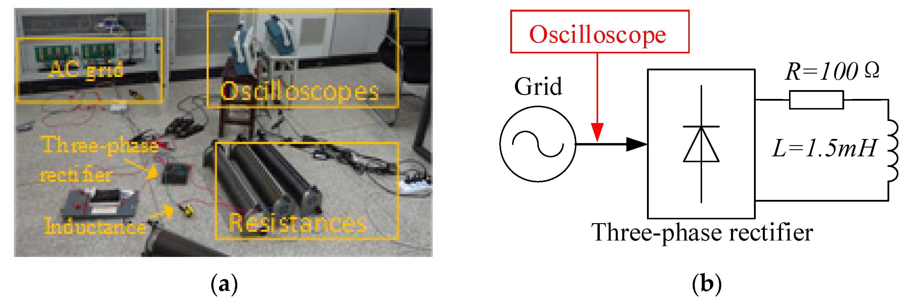
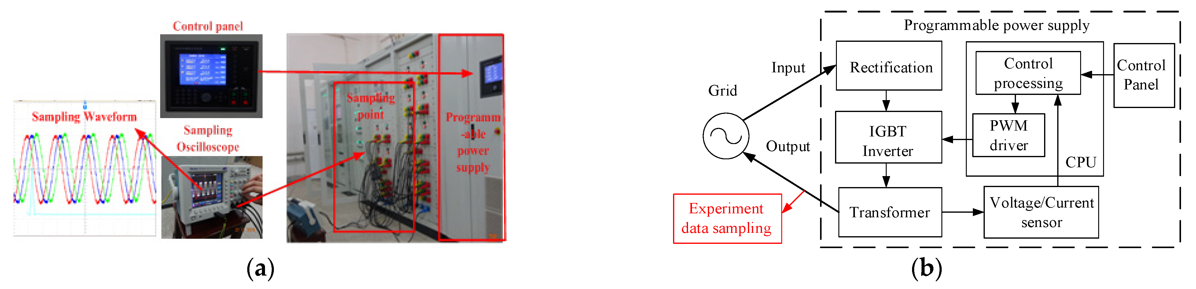
4.1.1. Experiment Settings

As an experimental example, we sample the AC distorted current signal. Experiment platform consists of AC grid (380 V, 50 Hz), oscilloscope (Tektronix GDS−2102) and nonlinear load (the three−phase rectifier, R = 100 Ω and L = 1.5 mH). It is shown in Figure 2. The AC current signals are sampled by the oscilloscope. Sampling cycles are selected as 10 µs and 40 µs. The experiment sampling current data and spectrogram are shown in Figure 3 and Figure 4. The HRI of harmonic components are measured to be approximately 24% of 5th, 10% of 7th, 10% of 11th, 5% of 13th, 5% of 17th, 4% of 19th by spectrum analysis.

HRI is defined as follows

$${\mathrm{HRI}}_{\mathrm{n}}=\frac{I_n}{I_1}\times 100\%$$

(28)

where $I_1$ is the voltage rms value of fundamental component, $I_n$ is the voltage rms value of n−th harmonic components.

The measurement noise covariance R of the algorithms is all selected as 0.06 A, that is the measurement error of the sensor. The initial covariance matrices are selected as $P_{0/0}=1000\times I_{14\times 14}$. The state noise covariance is selected as $Q_k=0.01\times I_{14\times 14}$ in (4). The state noise covariance is selected as $Q_k=0.01\times T\times I_{14\times 14}$ in (19).

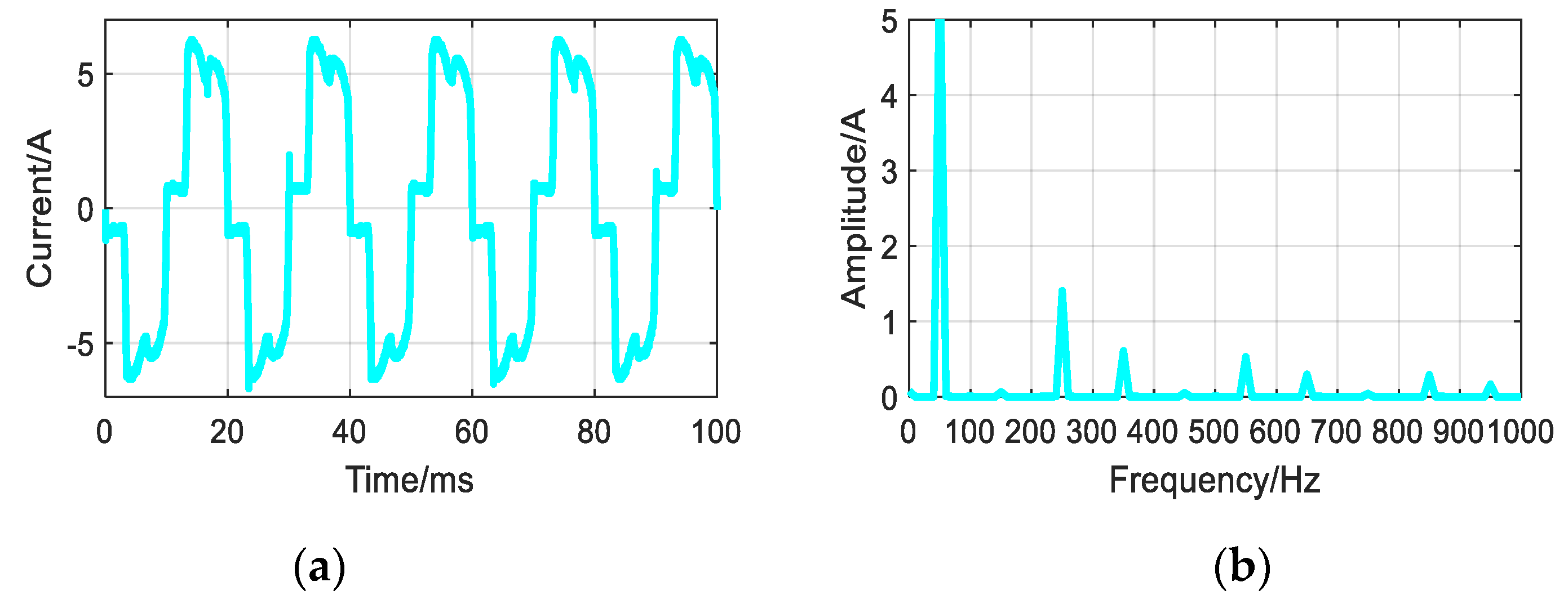
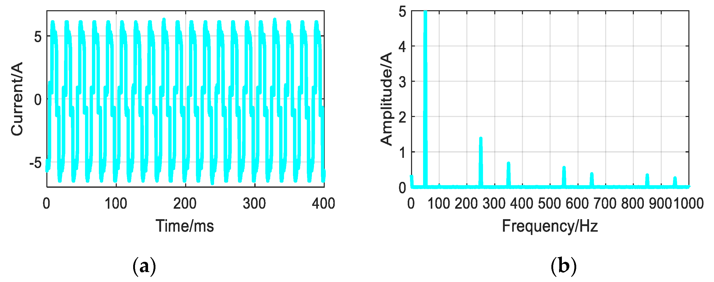
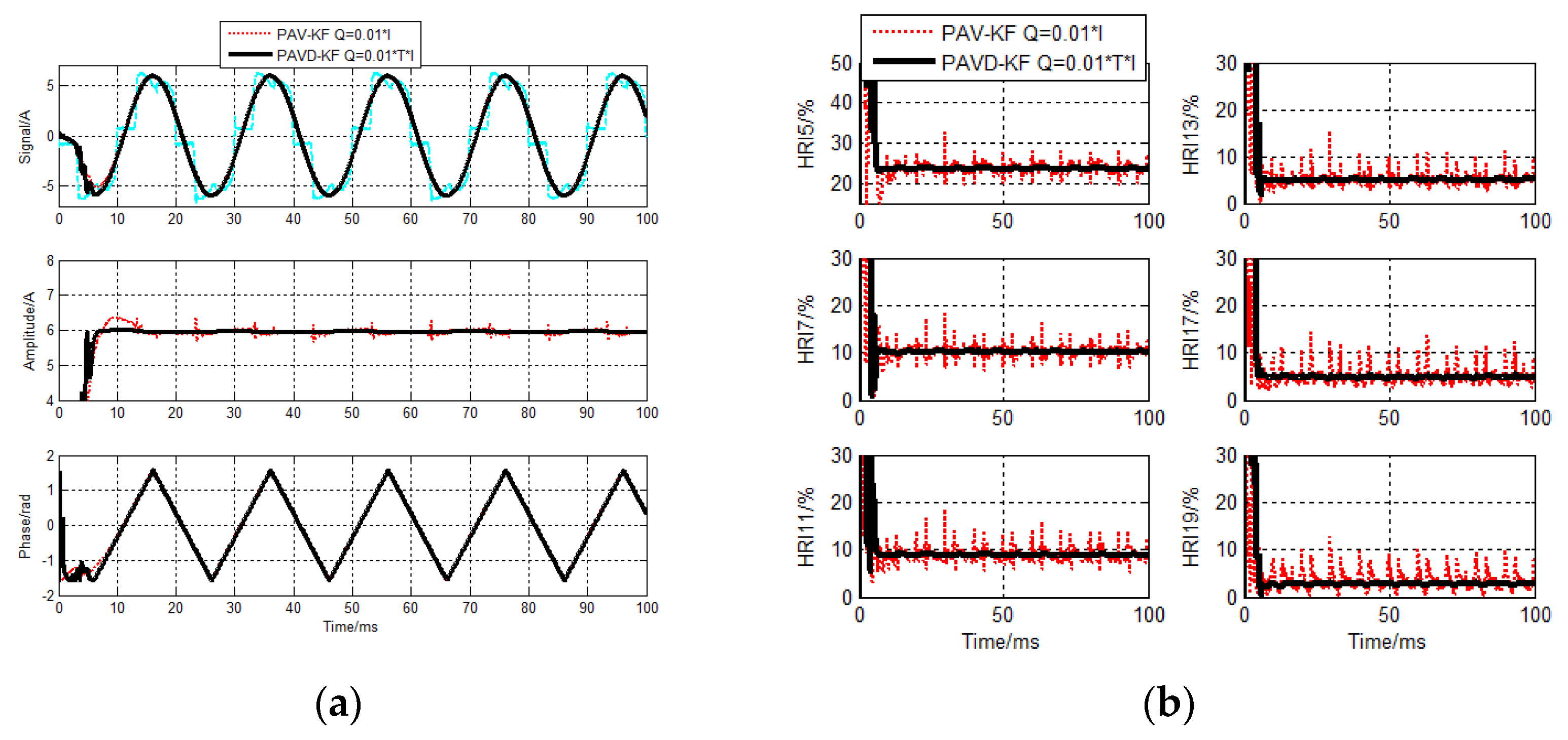
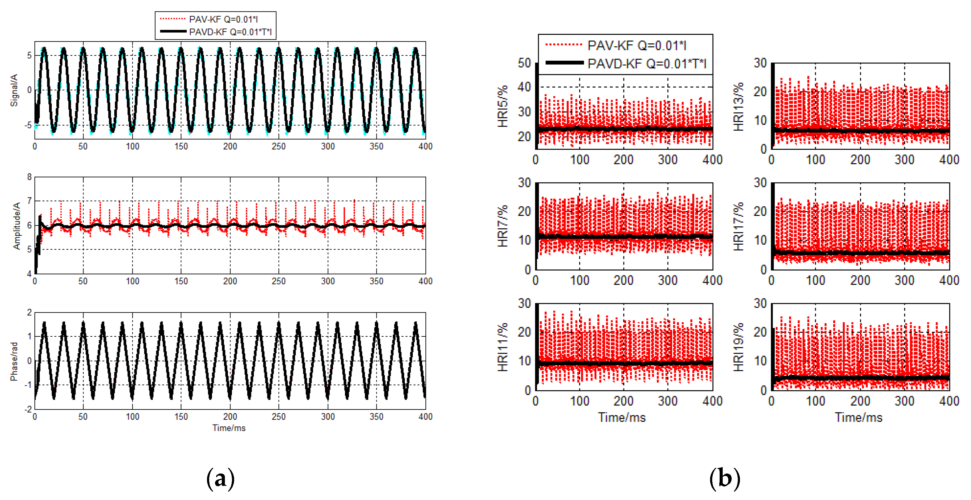
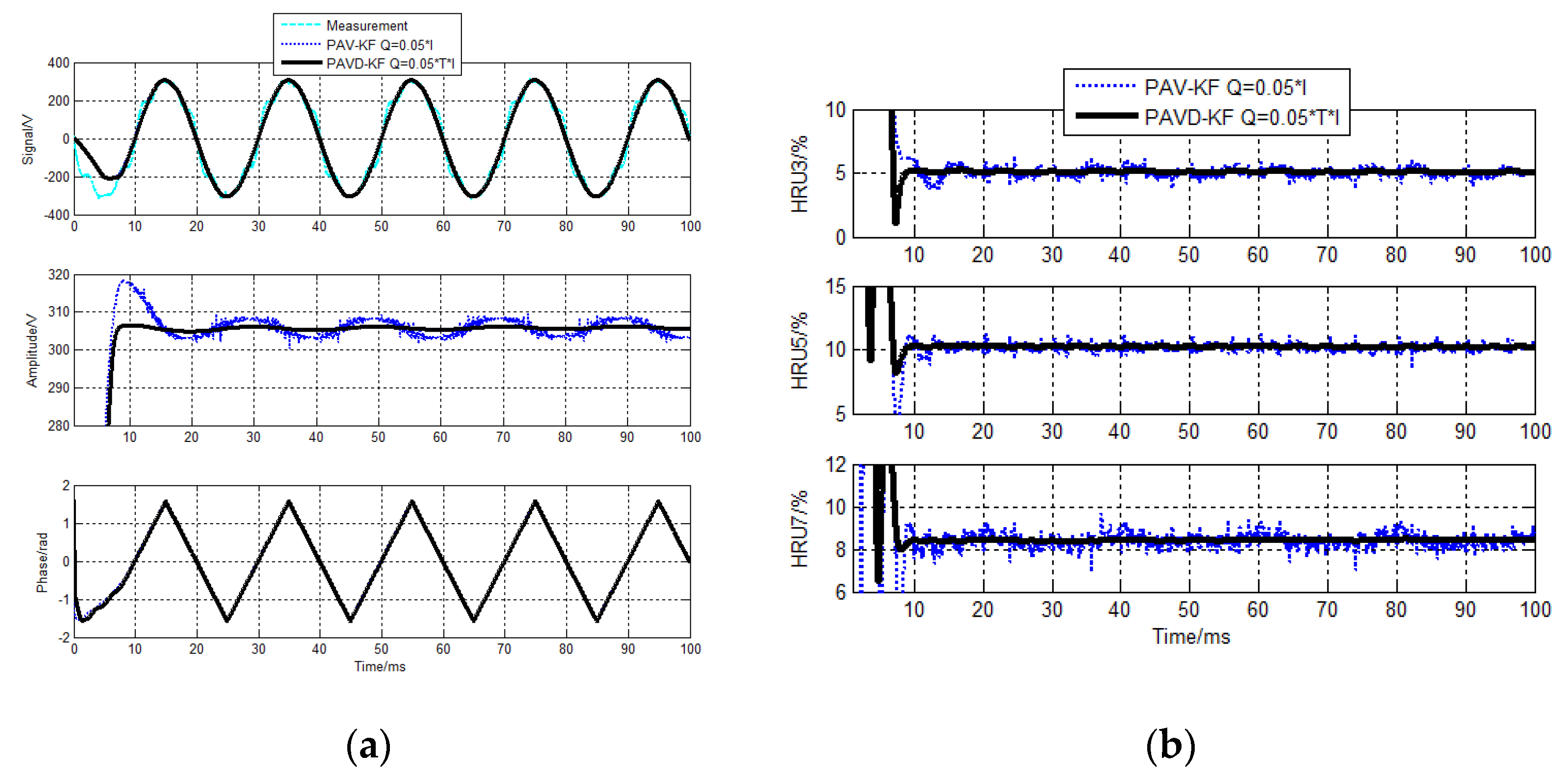
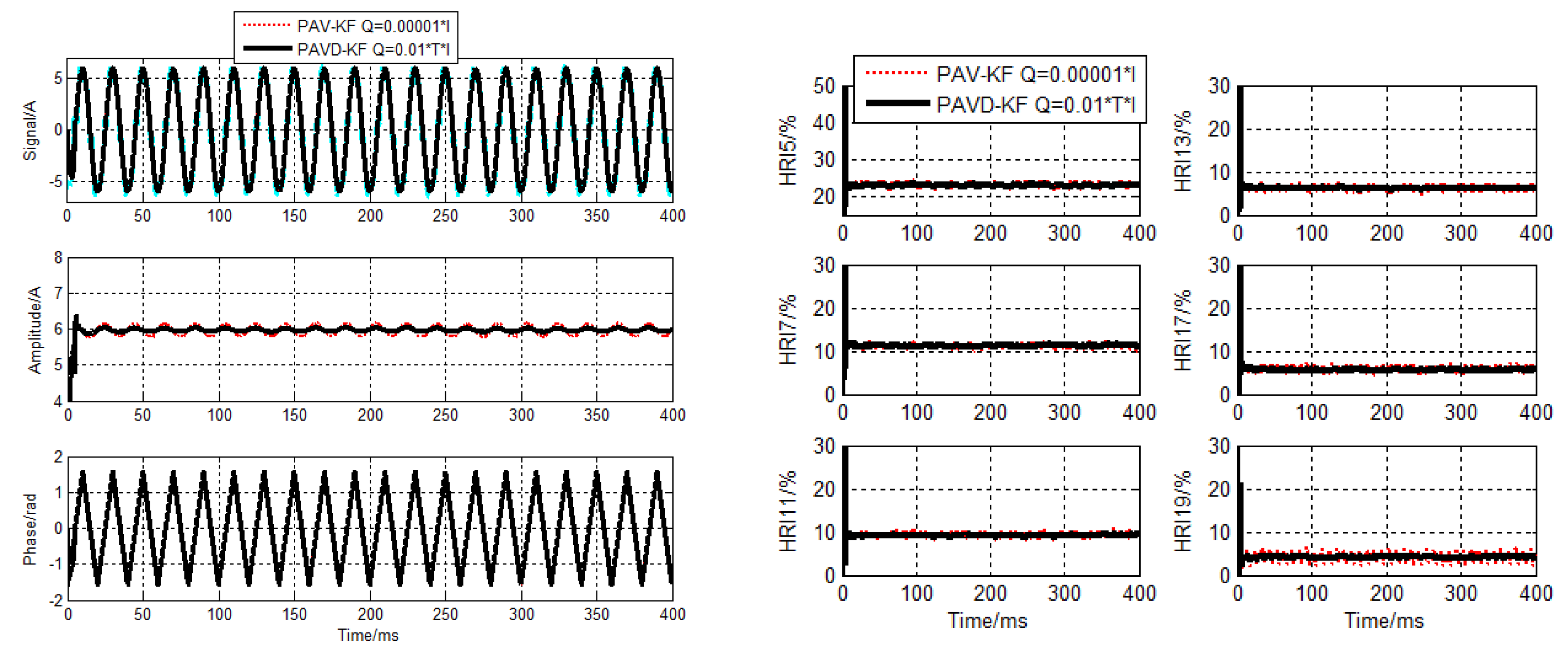
4.1.2. Detection Results for PAVD−KF Algorithm

Two algorithms of PAV−KF and PAVD−KF are evaluated and compared. The evaluation results for sampling cycle 10 µs and 40 µs are shown in Figure 5 and Figure 6.

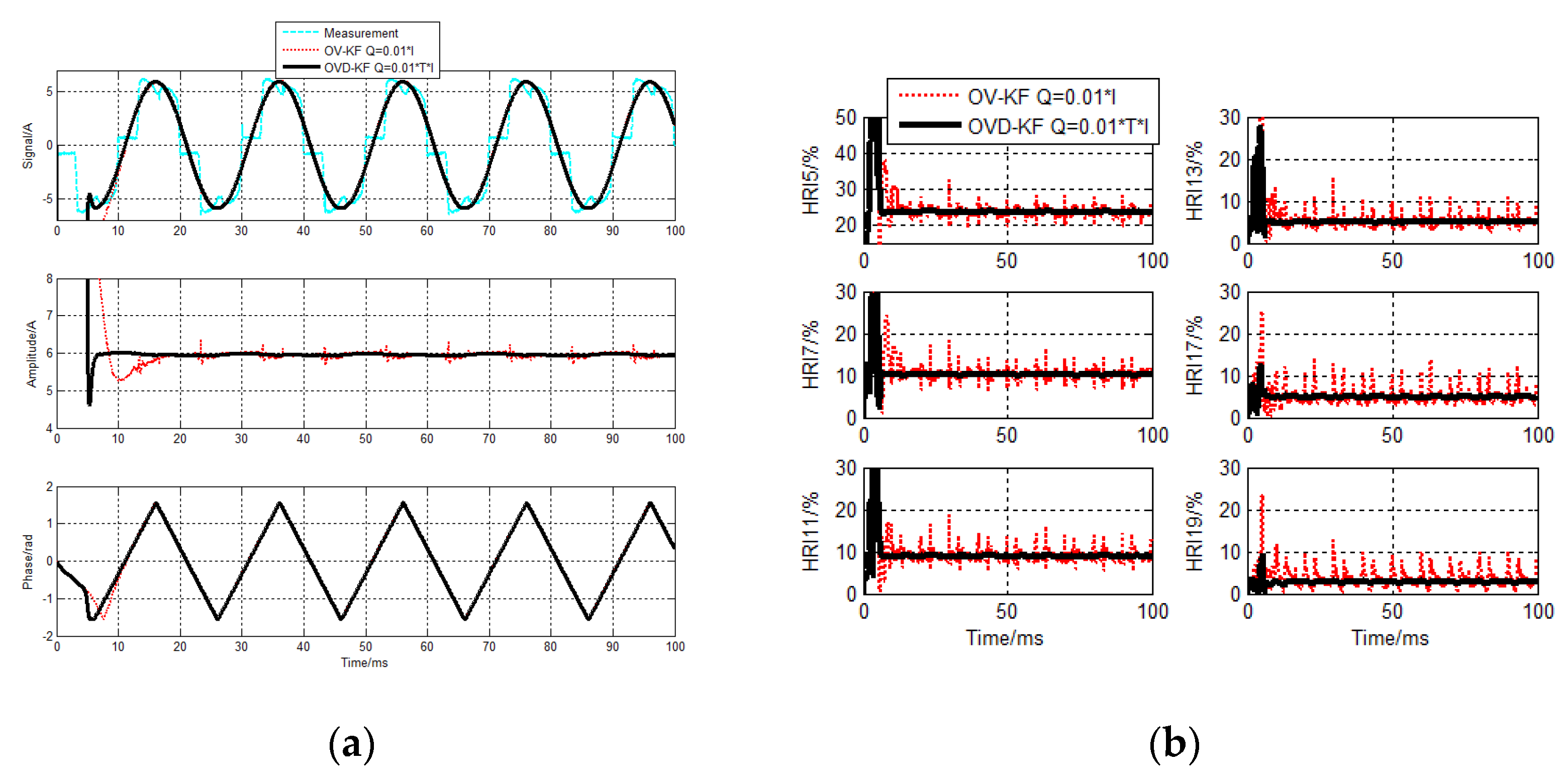
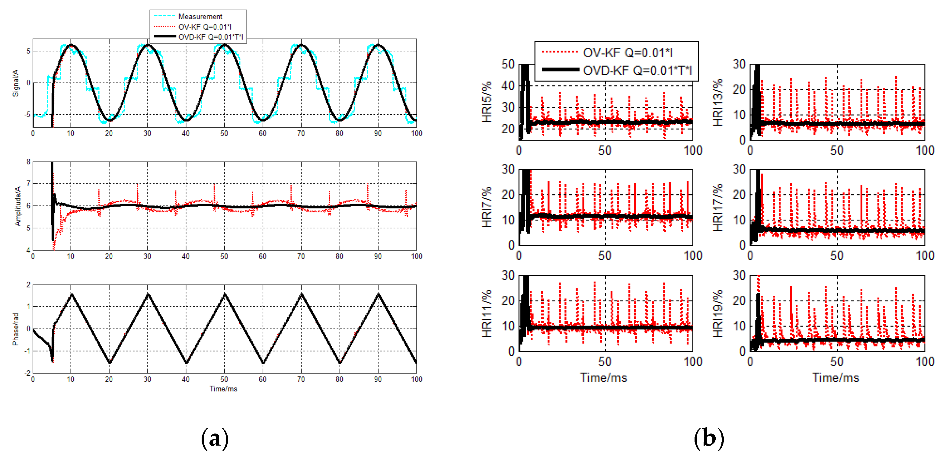
4.1.3. Detection Results for OVD−KF Algorithm

Two algorithms of OV−KF and OVD−KF are evaluated and compared. The evaluation results for sampling cycle 10 µs and 40 µs are shown in Figure 7 and Figure 8.

4.1.4. Summary for AC Current Detecting

It can be seen from Figure 5 and Figure 8, when Q = 0.01 × I, the detecting errors of the conventional PAV−KF and OV−KF algorithms are big. In particular, the detecting errors of the conventional algorithms for sampling cycle 40 μs are rather big. The errors are too big to affect the normal operation.

Corresponding to it, when Q combines with the sampling cycle, Q = 0.01 × T × I, regardless of the fundamental or harmonic components, the proposed detecting accuracies in PAVD−KF and OVD−KF algorithm are much higher than the conventional algorithms.

4.2. Experiment and Evaluation for AC Voltage Detection

4.2.1. Experiment Settings

The AC signal is grid voltage as an experimental example. Experiment platform is shown in Figure 9. The experiment of superimposing harmonics in fundamental voltage is carried out through a programmable power supply device. The AC voltage signals are sampled and the sampling cycles $T$ are selected by the oscilloscope of Tektronix GDS−2102.

The harmonics ratio for voltage (HRU) is defined as follows

$${\mathrm{HRU}}_{\mathrm{n}}=\frac{U_n}{U_1}\times 100\%$$

(29)

where $U_1$ is the voltage rms value of the fundamental component, and $U_n$ is the voltage rms value of n−th harmonic components.

Experiment voltage data for sampling cycle 10 µs is in Figure 10. Experiment voltage data for sampling cycle 40 µs is in Figure 11, and the HRU of harmonic components all are set as 5% of 3rd, 10% of 5th, and 8% of 7th.

The R of the algorithms are all selected as 3.11 V, that is the measurement error of the sensor. The initial covariance matrices of algorithms are selected as $P_{0/0}=1000\times I_{10\times 10}$. The state noise covariance matrix of algorithms is selected as $Q_k=0.05\times I_{10\times 10}$. The state noise covariance matrix of algorithms is $Q_k=0.1\times T\times I_{10\times 10}$.

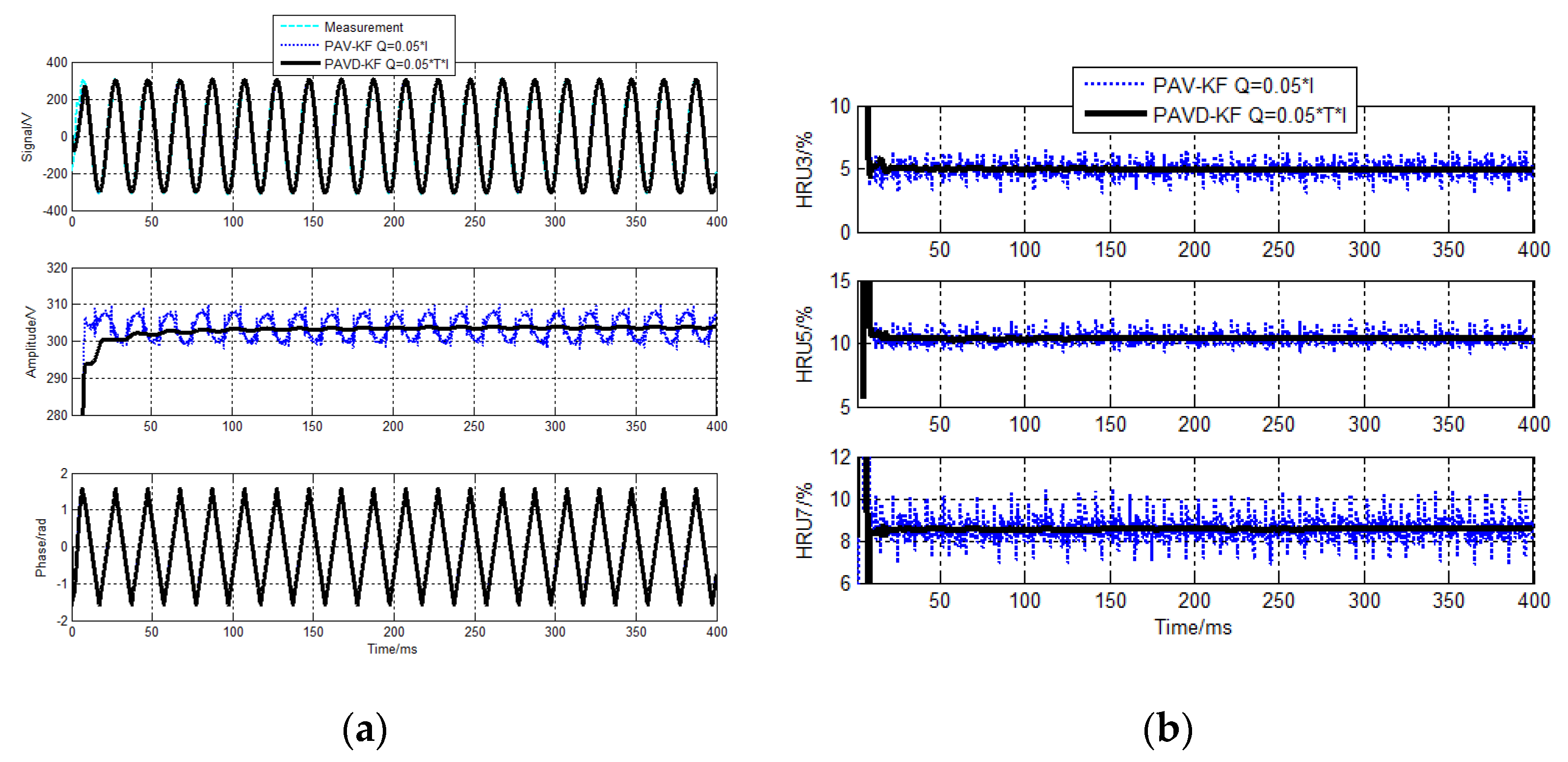
4.2.2. Detection Results for PAVD−KF Algorithm

PAVD−KF and PAV−KF algorithms are evaluated and compared. The detecting results of the sampling cycle 10 µs and 40 µs are shown in Figure 12 and Figure 13.

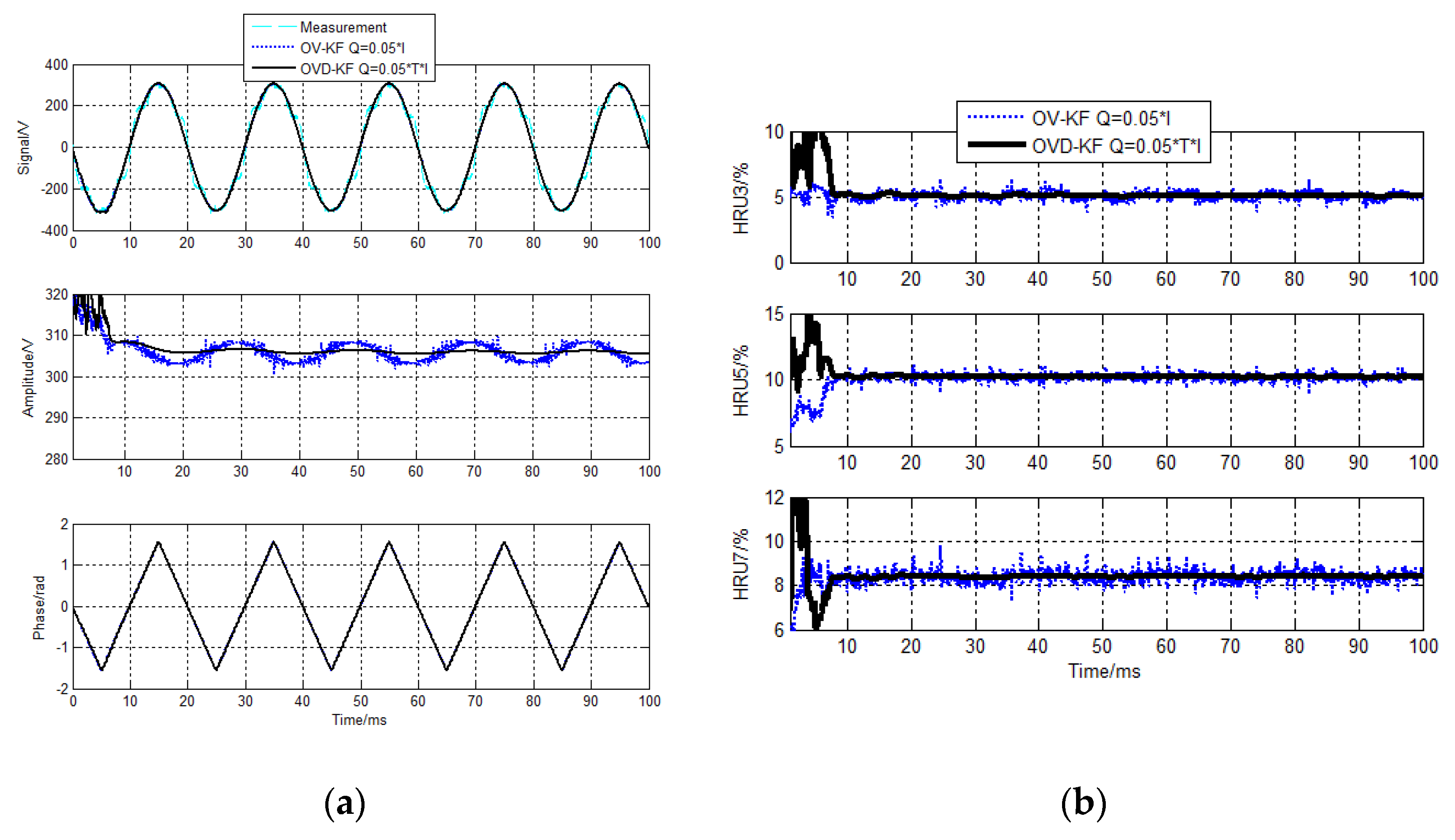
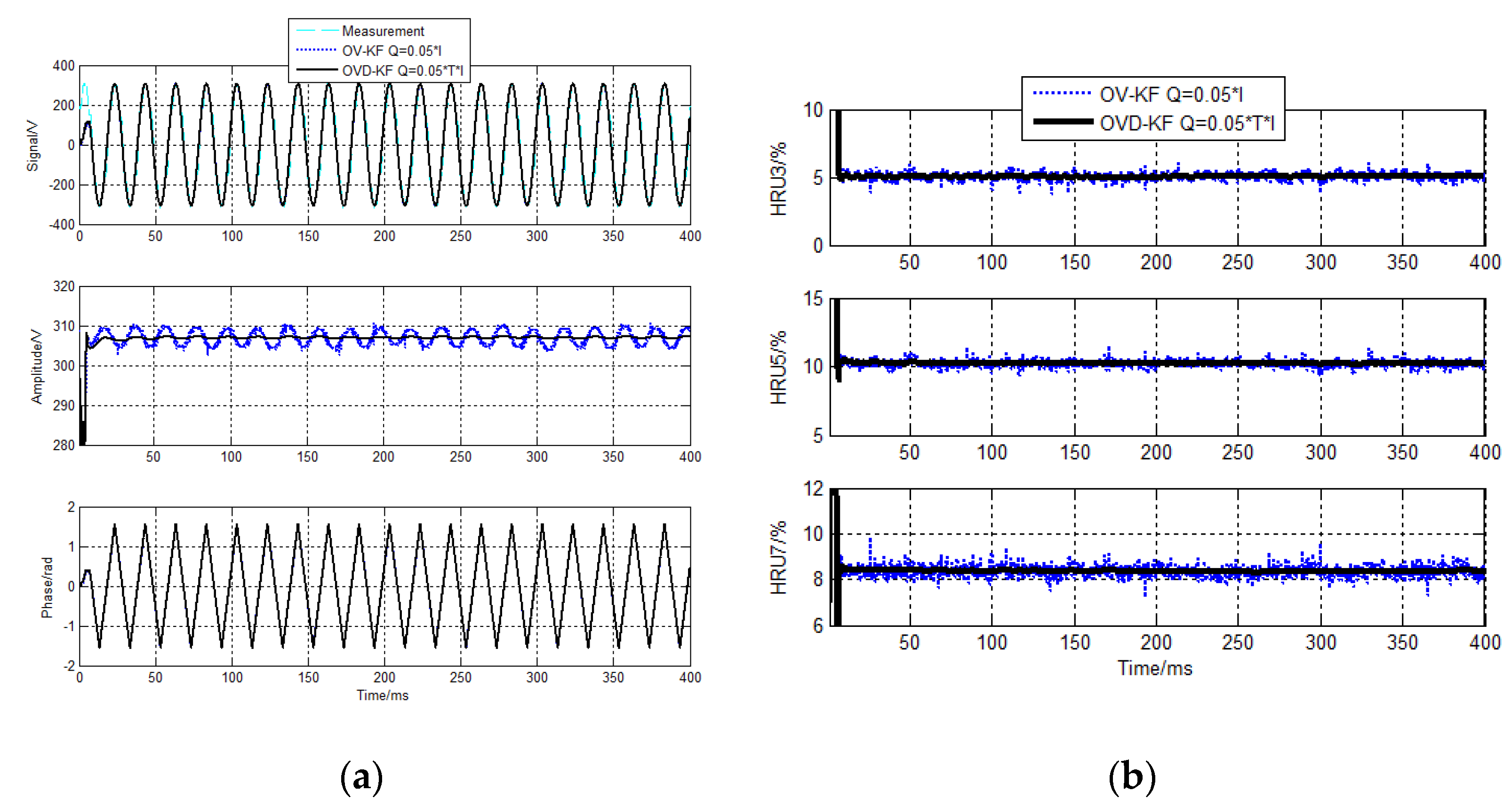
4.2.3. Detection Results for OVD−KF Algorithm

OVD−KF and OV−KF algorithms are evaluated and compared. The detecting results of the sampling cycle 10 µs and 40 µs are shown in Figure 14 and Figure 15.

4.2.4. Summary for AC Voltage Detecting

It can be seen from Figure 12 and Figure 13 that the amplitudes of the fundamental components of the conventional model−KF algorithm detecting are fluctuating, the stability of its detection shows poorly. Specifically, when we use the sampling cycle 40 µs, the error is too big to be ignored. From Figure 14 and Figure 15, we know that detecting errors of the harmonics components for the conventional OV−KF algorithm are also big, though the error seems smaller compared to PAV−KF. Corresponding to it, the detecting accuracies of the fundamental and harmonic components for the OVD−KF algorithm are higher than that of the OV−KF algorithm.

Generally, when Q = 0.05 × I, the conventional algorithms could basically meet the engineering requirements with some big errors under different sampling cycle conditions. When Q = 0.05 × T × I, all the novel algorithms could fulfill the requirements.

4.3. Summary for Experiment and Evaluation

In general, when using the fixed value, the error of PAV model is the biggest, neither current nor voltage can meet the demand. OV model performs better, when using the sampling cycle 10 µs, the voltage can be used normally, and the current error is too big to be used. But when using the sampling cycle 40 µs, both current and voltage cannot operate normally.

The proposed algorithms in this paper, whether it is PAVD model or OVD model, it is related to the sampling cycle, so the voltage and current detecting results can meet the engineering requirement.

Take PAV model with 40 μs in current and voltage tracking for example, the conventional methods produce big errors when Q = 0.01 × I detecting the current and Q = 0.05 × I detecting the voltage. Only when Q = 0.00001 × I detecting the current, the accuracy of it would be almost close to that of our proposed algorithm, as Figure 16 shows. When Q = 0.0005 × I detecting the voltage, the accuracy would satisfy the requirement, as Figure 17 shows.

5. Conclusions

This paper presents the PAVD−KF and OVD−KF algorithm derived from the stochastic process theory. It enhances the knowledge about the Kalman algorithms applied to the harmonic detection of the distorted AC grid. It gives a rule that the KF algorithms in the application of distorted grid AC signal detection is related to the sampling cycle and their state noise covariance cannot be simply considered as a constant.

This paper applies the actual current and voltage data of the sampling cycle 10 µs and 40 µs to detection and evaluation. The conventional algorithms have big errors in general and unable to meet engineering requirements. When using a fixed value of covariance, if we are going to obtain the ideal results, we need to spend a lot of time debugging (trying to make up) the parameters. Also, there is no theoretical source to set the fixed value of covariance. To solve it, we propose the algorithms to save much time and workload to get the ideal results. Besides, we make the algorithms more feasible and effective based on stochastic process theory. From which the results show that the proposed PAVD−KF and OVD−KF algorithms are effective and improve the dynamic detecting accuracy of grid AC signal significantly. This paper would provide a reference for the application of KF algorithms to harmonic detection, power quality control and grid synchronization in the future.

References

1. Auger, F.; Hilairet, M.; Guerrero, J.M.; Monmasson, E.; Orlowska-Kowalska, T.; Katsura, S. Industrial Applications of the Kalman Filter: A Review. IEEE Trans. Ind. Electron. 2013, 60, 5458–5471. [Google Scholar] [CrossRef] [Green Version]
2. Girgis, A.A.; Brown, R.G. Application of Kalman Filtering In Computer Relaying. IEEE Trans. Power Appar. Syst. 1981, 7, 3387–3397. [Google Scholar] [CrossRef]
3. Girgis, A.A.; Hwang, T.L.D. Optimal Estimation of Voltage Phasors and Frequency Deviation. IEEE Trans. Power Appar. Syst. 1984, 10, 2943–2951. [Google Scholar] [CrossRef]
4. Girgis, A.A.; Sallam, A.A.; El-Din, A.K. Identification and tracking of harmonic sources in a power system using a Kalman filte. IEEE Trans. Power Deliv. 1998, 13, 414–420. [Google Scholar] [CrossRef]
5. Nie, X. Detection of Grid Voltage Fundamental and Harmonic Components Using Kalman Filter Based on Dynamic Tracking Model. IEEE Trans. Ind. Electron. 2020, 67, 1191–1200. [Google Scholar] [CrossRef]
6. Naseri, F.; Kazemi, Z.; Farjah, E.; Ghanbari, T. Fast Detection and Compensation of Current Transformer Saturation Using Extended Kalman Filter. IEEE Trans. Power Deliv. 2020, 34, 1087–1097. [Google Scholar] [CrossRef]
7. Swain, S.; Subudhi, B. Grid Synchronization of a PV System with Power Quality Disturbances Using Unscented Kalman Filtering. IEEE Trans. Sustain. Energy 2019, 10, 1240–1247. [Google Scholar] [CrossRef]
8. Uz-Logoglu, E.; Salor, O.; Ermis, M. Real-Time Detection of Interharmonics and Harmonics of AC Electric Arc Furnaces on GPU Framework. IEEE Trans. Ind. Appl. 2019, 55, 1373–1378. [Google Scholar]
9. Xi, Y.; Tang, X.; Li, Z.; Cui, Y.; Zhao, T.; Zeng, X.; Guo, J.; Duan, W. Harmonic estimation in power systems using an optimised adaptive Kalman filter based on PSO-GA. IET Gener. Transm. Distrib. 2019, 13, 3968–3979. [Google Scholar] [CrossRef]
10. Bagheri, A.; Mardaneh, M.; Rajaei, A.; Rahideh, A. Detection of Grid Voltage Fundamental and Harmonic Components Using Kalman Filter and Generalized Averaging Method. IEEE Trans. Power Electron. 2016, 31, 1064–1073. [Google Scholar] [CrossRef]
11. Cardoso, R.; Camargo, R.F.; Pinheiro, H.; Grundling, H.A. Kalman filter based synchronisation methods. IET Gener. Transm. Distrib. 2008, 2, 542–555. [Google Scholar] [CrossRef]
12. Swain, S.; Subudhi, B. Iterated extended Kalman filter-based grid synchronisation control of a PV system. IET Energy Syst. Integr. 2019, 1, 219–228. [Google Scholar] [CrossRef]
13. Ferrero, R.; Pegoraro, P.A.; Toscani, S. Synchrophasor Estimation for Three-Phase Systems Based on Taylor Extended Kalman Filtering. IEEE Trans. Instrum. Meas. 2020, 69, 6723–6730. [Google Scholar] [CrossRef]
14. Golestan, S.; Guerrero, J.M.; Vasquez, J.C.; Abusorrah, A.M.; Al-Turki, Y. Single-Phase FLLs Based on Linear Kalman Filter, Limit-Cycle Oscillator, and Complex Bandpass Filter: Analysis and Comparison With a Standard FLL in Grid Applications. IEEE Trans. Power Electron. 2019, 34, 1064–1073. [Google Scholar] [CrossRef]
15. Ahmed, H.; Biricik, S.; Benbouzid, M. Linear Kalman Filter-Based Grid Synchronization Technique: An Alternative Implementation. IEEE Trans. Ind. Inform. 2021, 17, 3847–3856. [Google Scholar] [CrossRef]
16. Alam, S.J.; Arya, S.R. Control of UPQC based on steady state linear Kalman filter for compensation of power quality problems. Chin. J. Electr. Eng. 2020, 6, 52–65. [Google Scholar] [CrossRef]
17. Xi, Y.; Li, Z.; Zeng, X.; Tang, X.; Liu, Q.; Xiao, H. Detection of power quality disturbance using an adaptive process noise covariance Kalman filte. Digit. Signal Process. 2018, 76, 34–49. [Google Scholar] [CrossRef]
18. Wu, C.; Magana, M.E.; Cotilla-Sanchez, E. Dynamic Frequency and Amplitude Estimation for Three-Phase Unbalanced Power Systems Using the Unscented Kalman Filter. IEEE Trans. Instrum. Meas. 2019, 68, 3387–3395. [Google Scholar] [CrossRef]
19. Panigrahi, R.; Subudhi, B.; Panda, P.C. A robust LQG servo control strategy of shunt-active power filter for power quality enhancement. IEEE Trans. Power Electron. 2016, 31, 2860–2869. [Google Scholar] [CrossRef]
20. Panigrahi, R.; Subudhi, B. Performance enhancement of shunt active power filter using a Kalman filter-based H∞ control strategy. IEEE Trans. Power Electron. 2017, 32, 2622–2630. [Google Scholar] [CrossRef]
21. Abdelsalam, A.A.; Abdelaziz, A.Y.; Kamh, M.Z. A Generalized Approach for Power Quality Disturbances Recognition Based on Kalman Filter. IEEE Access 2021, 9, 93614–93628. [Google Scholar] [CrossRef]
22. Xi, Y.; Li, Z.; Tang, X.; Zeng, X. Classification of power quality disturbances based on KF-ML-Aided S-Transform and multilayers feedforward neural networks. IET Gener. Trans. Distrib. 2020, 14, 4010–4020. [Google Scholar] [CrossRef]
23. Abdelsalam, A.A.; Eldesouky, A.A.; Sallam, A.A. Classification of Power System Disturbances using Linear Kalman Filter and Fuzzy-expert System. Electr. Power Energy Syst. 2012, 43, 688–695. [Google Scholar] [CrossRef]
24. Abdelsalam, A.A.; Eldesouky, A.A.; Sallam, A.A. Characterization of power quality disturbances using hybrid technique of linear Kalman filter and fuzzy-expert system. Electr. Power Syst. Res. 2012, 83, 41–50. [Google Scholar] [CrossRef]
25. Brown, R.G.; Hwang, P.Y.C. Introduction to Random Signals and Applied Kalman Filtering with MATLAB Exercises, 4th ed.; John Wiley& Sons, Inc.: Hoboken, NJ, USA, 2011. [Google Scholar]
Figure 1. Diagram of the object circular movement being projected.
Energies 14 08175 g001
Figure 2. Experiment platform. (a) Current sampling experiment platform (b) Principle diagram of experiment platform.
Energies 14 08175 g002
Figure 3. Experiment current for sampling cycle 10 µs. (a) The sampling current data. (b) Spectrogram of sampling current data.
Energies 14 08175 g003
Figure 4. Experiment current for sampling cycle 40 µs. (a) The sampling current data. (b) Spectrogram of sampling current data.
Energies 14 08175 g004
Figure 5. PAVD−KF current detecting results for sampling cycle 10 µs. (a) Fundamental components detecting results (b) HRI detecting results.
Energies 14 08175 g005
Figure 6. PAVD−KF current detecting results for sampling cycle 40 µs. (a) Fundamental components detecting results (b) HRI detecting results.
Energies 14 08175 g006
Figure 7. OVD−KF current detecting results for sampling cycle 10 µs. (a) Fundamental components detecting results (b) HRI detecting results.
Energies 14 08175 g007
Figure 8. OVD−KF current detecting results for sampling cycle 40 µs. (a) Fundamental components detecting results (b) HRI detecting results.
Energies 14 08175 g008
Figure 9. Experiment platform. (a) Voltage sampling experiment platform. (b) Principle diagram of experiment platform.
Energies 14 08175 g009
Figure 10. Experiment voltage for sampling cycle 10 µs. (a) The sampling voltage data. (b) Spectrogram of sampling voltage data.
Energies 14 08175 g010
Figure 11. Experiment voltage for sampling cycle 40 µs. (a) The sampling voltage data. (b) Spectrogram of sampling voltage data.
Energies 14 08175 g011
Figure 12. PAVD−KF voltage detecting results for sampling cycle 10 µs. (a) Fundamental components detecting results (b) HRU detecting results.
Energies 14 08175 g012
Figure 13. PAVD−KF voltage detecting results for sampling cycle 40 µs. (a) Fundamental components detecting results (b) HRU detecting results.
Energies 14 08175 g013
Figure 14. OVD−KF voltage detecting results for sampling cycle 10 µs. (a) Fundamental components detecting results (b) HRU detecting results.
Energies 14 08175 g014
Figure 15. OVD−KF voltage detecting results for sampling cycle 40 µs. (a) Fundamental components detecting results (b) HRU detecting results.
Energies 14 08175 g015
Figure 16. PAVD−KF current detecting results for sampling cycle 40 µs. (Q = 0.00001 × I).
Energies 14 08175 g016
Figure 17. PAVD−KF voltage detecting results for sampling cycle 40 µs. (Q = 0.0005 × I).
Energies 14 08175 g017
Publisher’s Note: MDPI stays neutral with regard to jurisdictional claims in published maps and institutional affiliations.