
A Case Study on the Closed-Type Barrier Effect on Debris Flows at Mt. Woomyeon, Korea in 2011 via a Numerical Approach


Abstract
:1. Introduction
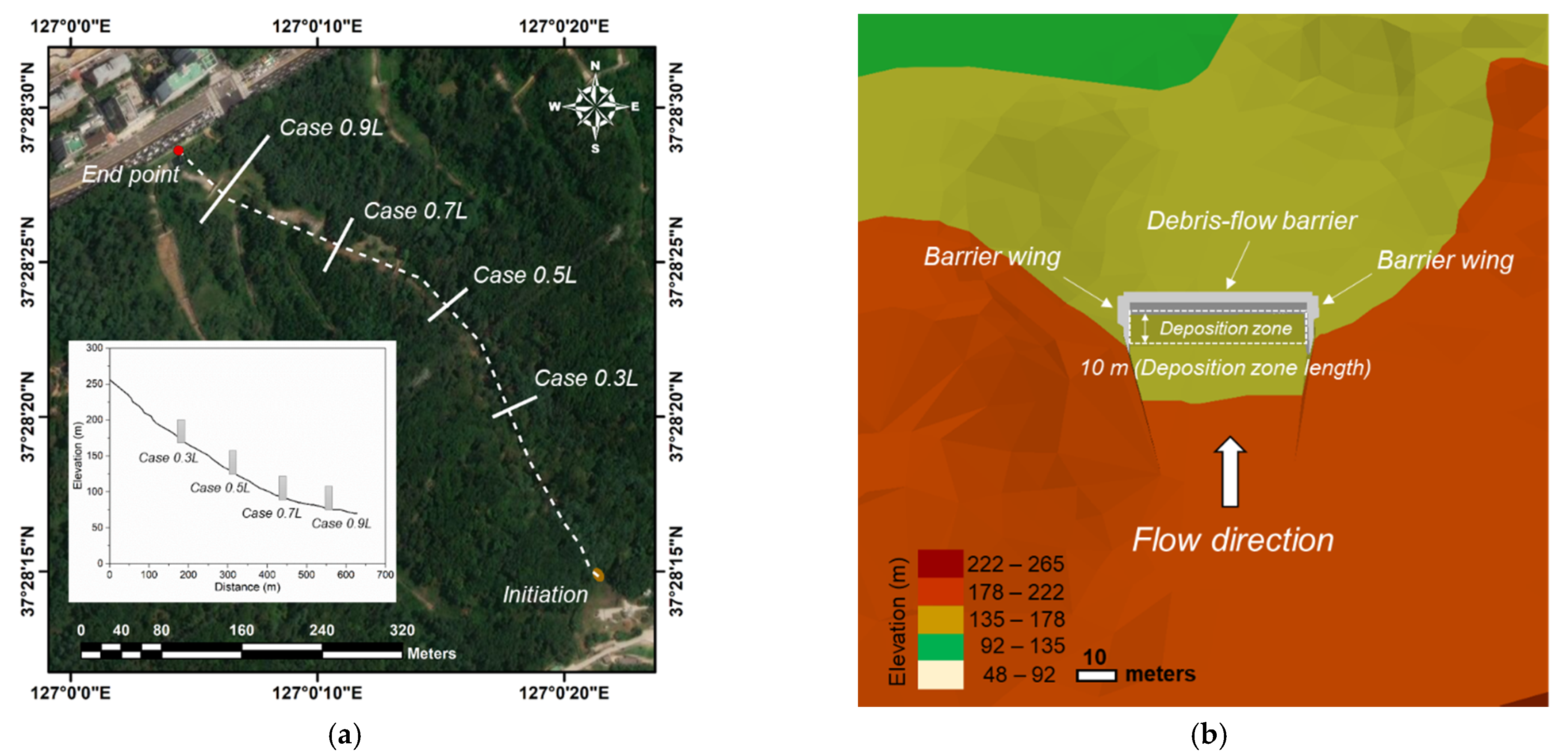
2. Study Area
3. Study Method
3.1. Numerical Code
3.2. Rheological Model
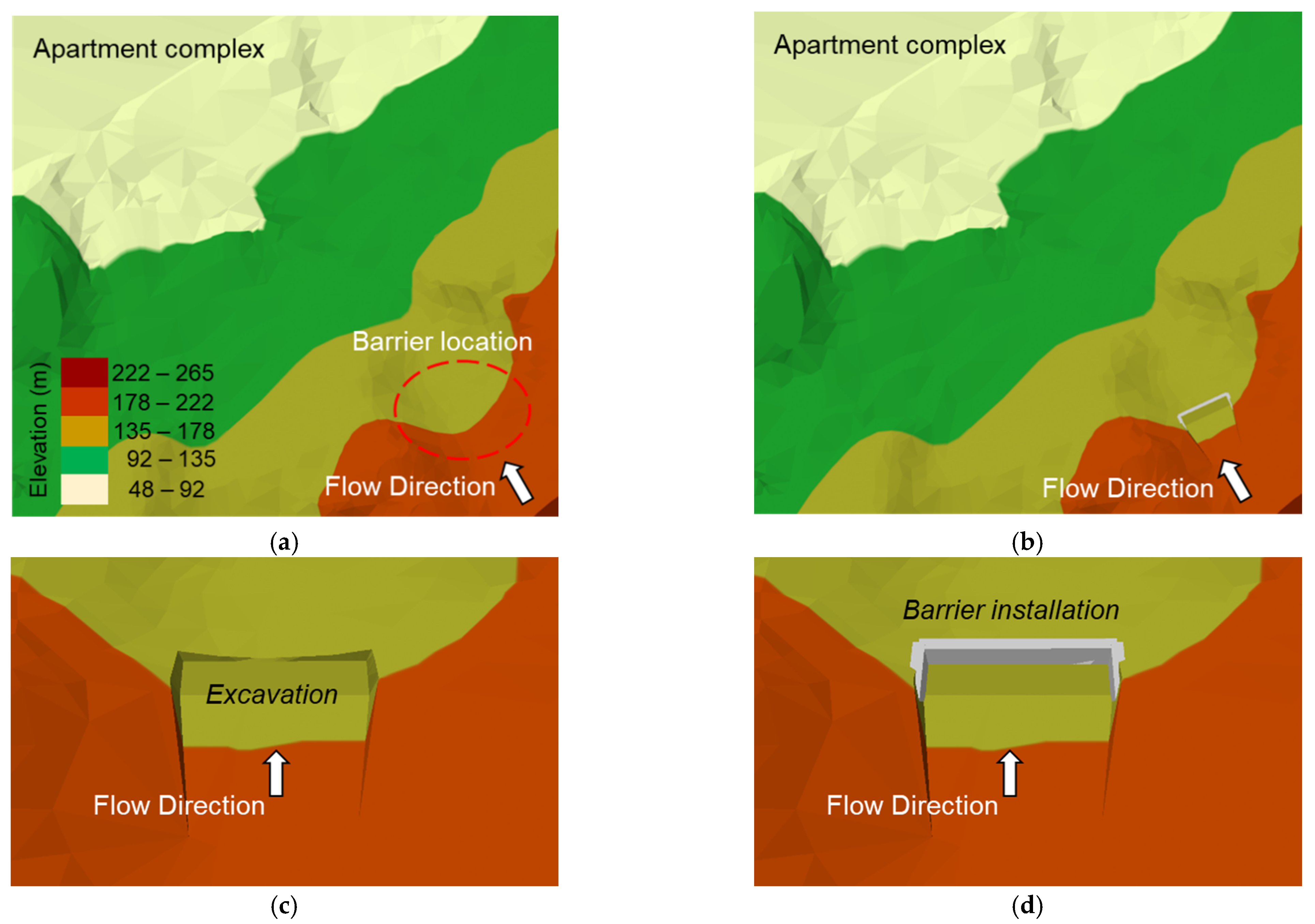
3.3. Barrier Installation
3.4. Deposition Zone at the Upstream Face of a Barrier
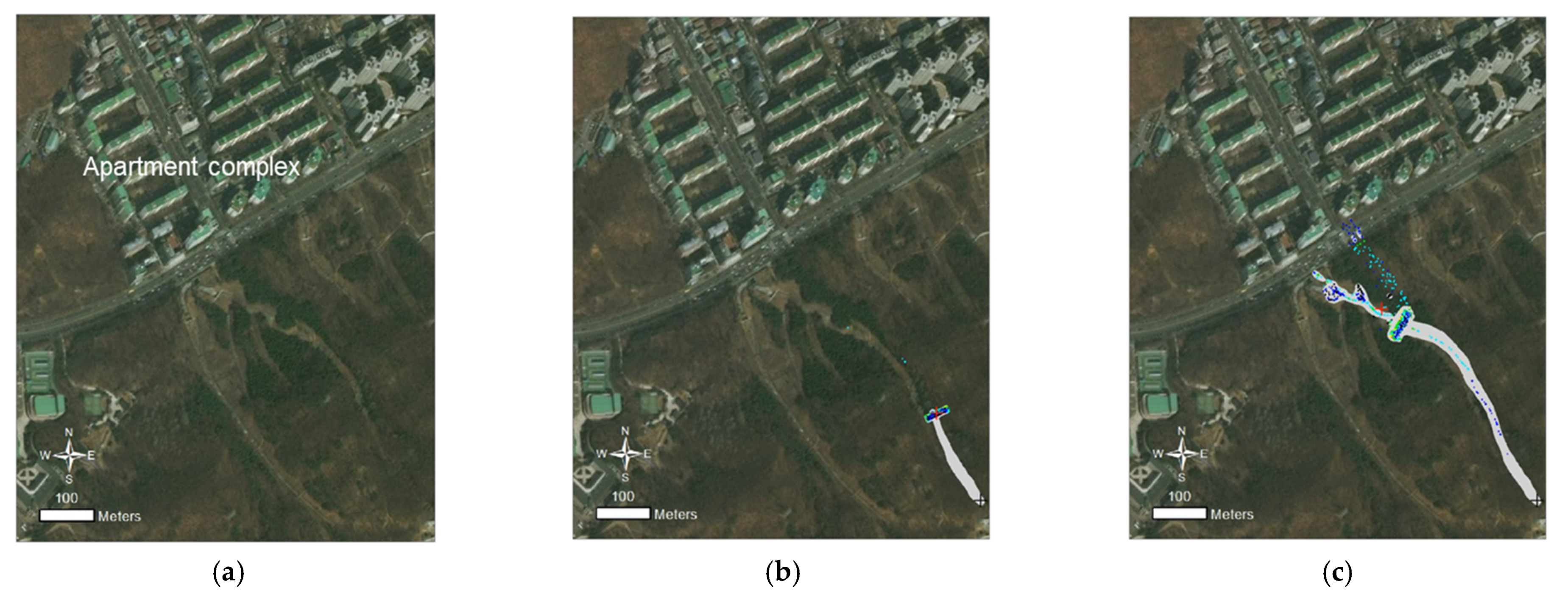
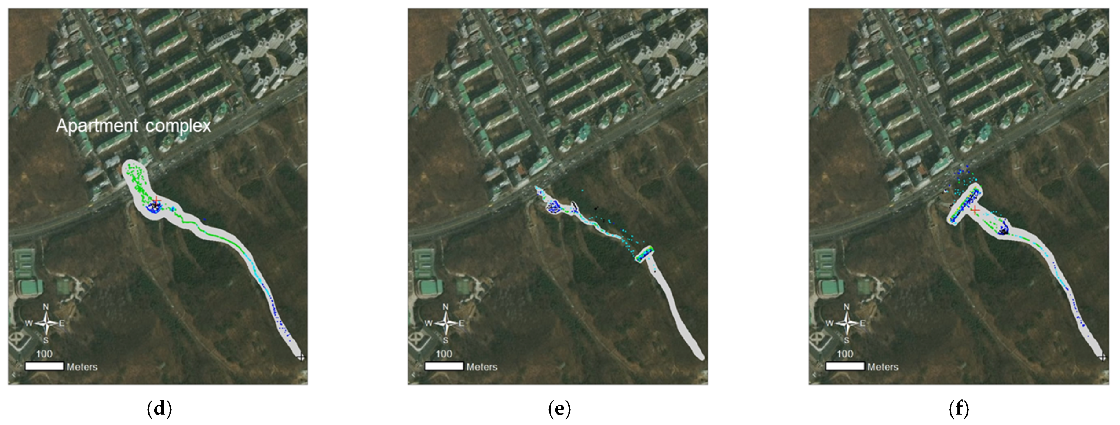
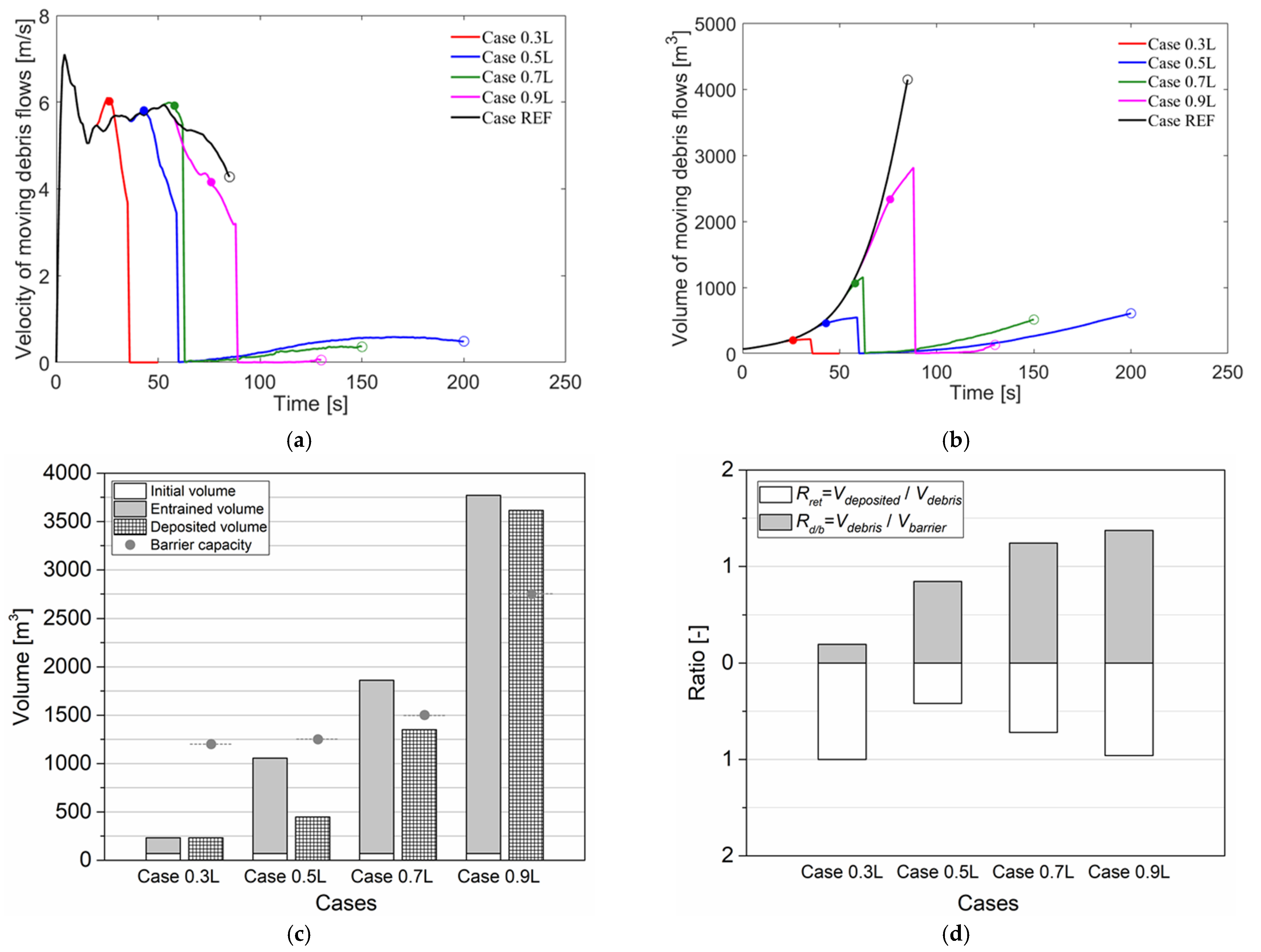
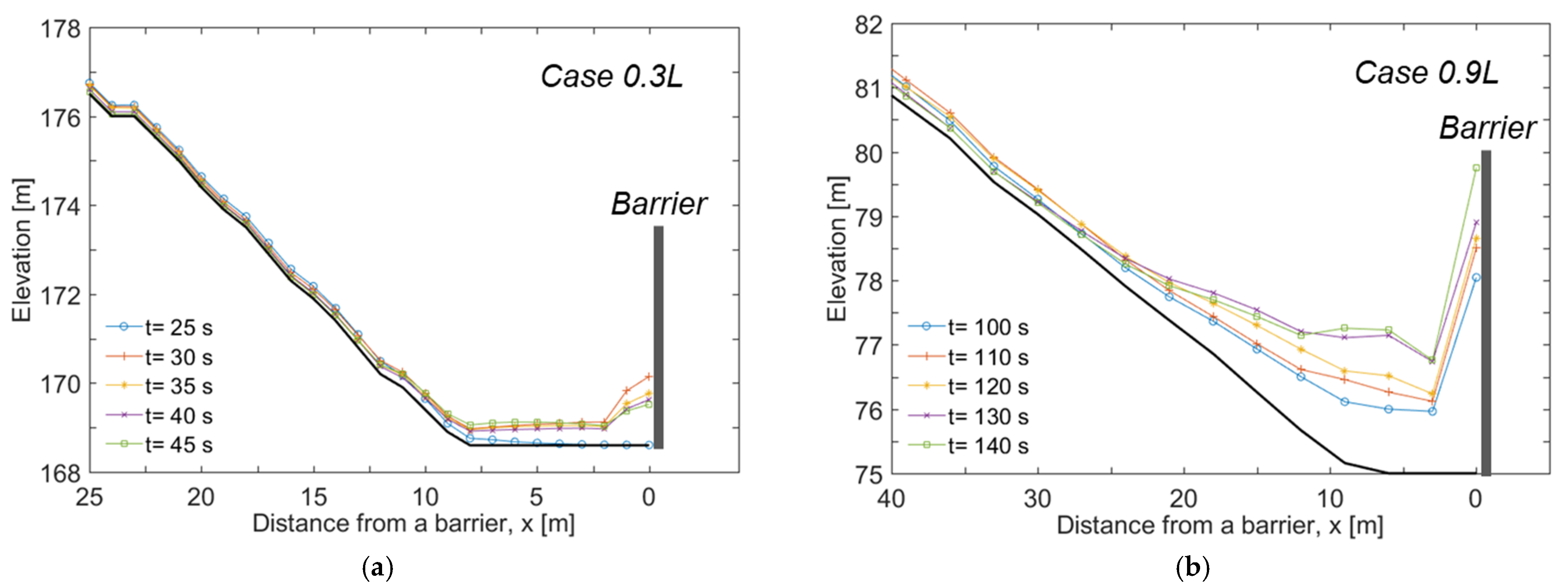
4. Results and Analysis
5. Discussion and Implication
6. Conclusions
Author Contributions
Funding
Data Availability Statement
Conflicts of Interest
References
- Jakob, M.; Hungr, O. Debris Flow Hazards and Related Phenomena; Springer: Berlin/Heidelberg, Germany, 2005. [Google Scholar]
- Tang, C.; Zhu, J.; Chang, M.; Ding, J.; Qi, X. An empirical–statistical model for predicting debris flow run-out zones in the Wenchuan earthquake area. Quat. Int. 2012, 250, 63–73. [Google Scholar] [CrossRef]
- Shen, W.; Wang, D.; Qu, H.; Li, T. The effect of check dams on the dynamic and bed entrainment processes of debris flows. Landslides 2019, 16, 2201–2217. [Google Scholar] [CrossRef]
- Orense, R.P.; Sapuay, S.E. Preliminary report on the 17 February 2006 Leyte, Philippines landslide. Soils Found. 2006, 46, 685–693. [Google Scholar] [CrossRef] [Green Version]
- Yune, C.Y.; Chae, Y.K.; Paik, J.; Kim, G.; Lee, S.W.; Seo, H.S. Debris flow in metropolitan area—2011 Seoul debris flow. J. Mt. Sci. 2013, 10, 199–206. [Google Scholar] [CrossRef]
- Jeong, S.; Kim, Y.; Lee, J.K.; Kim, J. The 27 July 2011 debris flows at Umyeonsan, Seoul, Korea. Landslides 2015, 12, 799–813. [Google Scholar] [CrossRef]
- Wenbing, H.; Guoqiang, O. Efficiency of slit dam prevention against non-viscous debris flow. Wuhan Univ. J. Nat. Sci. 2006, 11, 865–869. [Google Scholar] [CrossRef]
- Kim, Y.; Nakagawa, H.; Kawaike, K.; Zhang, H. Study on Characteristic Analysis of Closed-Type Sabo Dam with a Flap due to Dynamic Force of Debris Flow; Kyoto University: Kyoto, Japan, 2013; pp. 503–522. [Google Scholar]
- Ng, C.W.; Choi, C.; Song, D.; Kwan, J.; Koo, R.; Shiu, H.; Ho, K.K. Physical modeling of baffles influence on landslide debris mobility. Landslides 2015, 12, 1–18. [Google Scholar] [CrossRef]
- Wendeler, C.; Volkwein, A. Laboratory tests for the optimization of mesh size for flexible debris-flow barriers. Nat. Hazards Earth Syst. Sci. 2015, 15, 2597–2604. [Google Scholar] [CrossRef] [Green Version]
- Choi, S.K.; Lee, J.M.; Kwon, T.H. Effect of slit-type barrier on characteristics of water-dominant debris flows: Small-scale physical modeling. Landslides 2018, 15, 111–122. [Google Scholar] [CrossRef]
- Choi, S.K.; Park, J.Y.; Lee, D.H.; Lee, S.R.; Kim, Y.T.; Kwon, T.H. Assessment of barrier location effect on debris flow based on smoothed particle hydrodynamics (SPH) simulation on 3D terrains. Landslides 2021, 18, 217–234. [Google Scholar] [CrossRef]
- O’Brien, J.S.; Julien, P.Y.; Fullerton, W.T. Two-dimensional water flood and mudflow simulation. J. Hydraul. Eng. 1993, 119, 244–261. [Google Scholar] [CrossRef]
- McDougall, S.; Hungr, O. A model for the analysis of rapid landslide motion across three-dimensional terrain. Can. Geotech. J. 2004, 41, 1084–1097. [Google Scholar] [CrossRef]
- Pirulli, M.; Mangeney, A. Results of back-analysis of the propagation of rock avalanches as a function of the assumed rheology. Rock Mech. Rock Eng. 2008, 41, 59–84. [Google Scholar] [CrossRef]
- Beguería, S.; Van Asch, T.W.; Malet, J.P.; Gröndahl, S. A GIS-based numerical model for simulating the kinematics of mud and debris flows over complex terrain. Nat. Hazards Earth Syst. Sci. 2009, 9, 1897–1909. [Google Scholar] [CrossRef] [Green Version]
- Pastor, M.; Haddad, B.; Sorbino, G.; Cuomo, S.; Drempetic, V. A depth-integrated, coupled SPH model for flow-like landslides and related phenomena. Int. J. Numer. Anal. Methods Geomech. 2009, 33, 143–172. [Google Scholar] [CrossRef]
- Christen, M.; Kowalski, J.; Bartelt, P. RAMMS: Numerical simulation of dense snow avalanches in three-dimensional terrain. Cold Reg. Sci. Technol. 2010, 63, 1–14. [Google Scholar] [CrossRef] [Green Version]
- Quan, L. Dynamic Numerical Run-Out Modeling for Quantitative Landslide Risk Assessment. Ph.D. Thesis, University of Twente, Enschede, The Netherlands, 2012. [Google Scholar]
- Osti, R.; Egashira, S. Method to improve the mitigative effectiveness of a series of check dams against debris flows. Hydrol. Process. Int. J. 2008, 22, 4986–4996. [Google Scholar] [CrossRef]
- Korean Society of Civil Engineers (KSCE). Research Contract Report: Causes Survey and Restoration Work of Mt. Woomyeon Landslide; Korean Society of Civil Engineers: Seoul, Korea, 2012. [Google Scholar]
- National Geographic Information Institute of Korea (NGII). Digital Elevation Maps of South Jeolla Province with the Scale of 1:5000; National Geographic Information Institute of Korea: Suwon, Korea, 2010.
- McDougall, S. 2014 Canadian Geotechnical Colloquium: Landslide runout analysis—Current practice and challenges. Can. Geotech. J. 2017, 54, 605–620. [Google Scholar] [CrossRef] [Green Version]
- McDougall, S.; Hungr, O. Dynamic modelling of entrainment in rapid landslides. Can. Geotech. J. 2005, 42, 1437–1448. [Google Scholar] [CrossRef]
- Hungr, O. A model for the run-out analysis of rapid flow slides, debris flows, and avalanches. Can. Geotech. J. 1995, 32, 610–623. [Google Scholar] [CrossRef]
- Voellmy, A. Über die Zerstörungskraft von Lawinen. Schweiz. Bauztg. 1955, 73, 212–285. [Google Scholar]
- Cepeda, J.; Chávez, J.A.; Martínez, C.C. Procedure for the selection of runout model parameters from landslide back-analyses: Application to the Metropolitan Area of San Salvador, El Salvador. Landslides 2010, 7, 105–116. [Google Scholar] [CrossRef]
- Aaron, J.; McDougall, S.; Nolde, N. Two methodologies to calibrate landslide runout models. Landslides 2019, 16, 907–920. [Google Scholar] [CrossRef]
- McDougall, S. A New Continuum Dynamic Model for the Analysis of Extremely Rapid Landslide Motion across Complex 3D Terrain. Ph.D. Thesis, University of British Columbia, Vancouver, BC, Canada, 2006. [Google Scholar]
- Ng, C.W.W.; Choi, C.E.; Kwan, J.S.H.; Koo, R.C.H.; Shiu, H.Y.K.; Ho, K.K.S. Effects of baffle transverse blockage on landslide debris impedance. Procedia Earth Planet. Sci. 2014, 9, 3–13. [Google Scholar] [CrossRef] [Green Version]
- Zhou, G.G.D.; Song, D.; Choi, C.E.; Pasuto, A.; Sun, Q.C.; Dai, D.F. Surge impact behavior of granular flows: Effects of water content. Landslides 2018, 15, 695–709. [Google Scholar] [CrossRef]
- Song, D.; Choi, C.E.; Ng, C.W.W.; Zhou, G.G.; Kwan, J.S.; Sze, H.Y.; Zheng, Y. Load-attenuation mechanisms of flexible barrier subjected to bouldery debris flow impact. Landslides 2019, 16, 2321–2334. [Google Scholar] [CrossRef]
- Siyou, X.; Lijun, S.; Yuanjun, J.; Xin, Q.; Min, X.; Xiaobo, H.; Zhenyu, L. Experimental investigation on the impact force of the dry granular flow against a flexible barrier. Landslides 2020, 17, 1465–1483. [Google Scholar] [CrossRef]
- Tan, D.Y.; Yin, J.H.; Qin, J.Q.; Zhu, Z.H.; Feng, W.Q. Experimental study on impact and deposition behaviours of multiple surges of channelized debris flow on a flexible barrier. Landslides 2020, 17, 1577–1589. [Google Scholar] [CrossRef]
- Remaître, A.; Van Asch, T.W.; Malet, J.P.; Maquaire, O. Influence of check dams on debris-flow run-out intensity. Nat. Hazards Earth Syst. Sci. 2008, 8, 1403–1416. [Google Scholar] [CrossRef]
- Iverson, R.M.; George, D.L.; Logan, M. Debris flow runup on vertical barriers and adverse slopes. J. Geophys. Res. Earth Surf. 2016, 121, 2333–2357. [Google Scholar] [CrossRef]
- Revellino, P.; Hungr, O.; Guadagno, F.M.; Evans, S.G. Velocity and runout simulation of destructive debris flows and debris avalanches in pyroclastic deposits, Campania region, Italy. Environ. Geol. 2004, 45, 295–311. [Google Scholar] [CrossRef]
- Hungr, O.; Evans, S.G. Entrainment of debris in rock avalanches: An analysis of a long run-out mechanism. Geol. Soc. Am. Bull. 2004, 116, 1240–1252. [Google Scholar] [CrossRef]
- Dai, Z.; Huang, Y.; Cheng, H.; Xu, Q. SPH model for fluid–structure interaction and its application to debris flow impact estimation. Landslides 2017, 14, 917–928. [Google Scholar] [CrossRef]
- Chen, H.X.; Li, J.; Feng, S.J.; Gao, H.Y.; Zhang, D.M. Simulation of interactions between debris flow and check dams on three-dimensional terrain. Eng. Geol. 2019, 251, 48–62. [Google Scholar] [CrossRef]


| Parameters/Cases | Site | ||
|---|---|---|---|
| Input parameters | Unit weight | 16.3 kN/m3 | |
| Internal friction angle | 40° | ||
| Erosion rate | 7.8 × 10⁻³ %/m | ||
| Maximum erosion depth | 1.6 m | ||
| Friction coefficient | 0.03 | ||
| Turbulence parameter | 800 m/s2 | ||
| Debris volume | Source volume | Field | 70 m3 |
| DAN3D | 70 m3 | ||
| Final volume | Field | 3914 m3 | |
| DAN3D | 4024 m3 | ||
| Barrier condition | Width | Distance fromthe initiation location | |
| Case REF | 627 m | ||
| Case 0.3 L | 48 m | 189 m | |
| Case 0.5 L | 50 m | 311 m | |
| Case 0.7 L | 60 m | 437 m | |
| Case 0.9 L | 110 m | 563 m | |
Publisher’s Note: MDPI stays neutral with regard to jurisdictional claims in published maps and institutional affiliations. |
© 2021 by the authors. Licensee MDPI, Basel, Switzerland. This article is an open access article distributed under the terms and conditions of the Creative Commons Attribution (CC BY) license (https://creativecommons.org/licenses/by/4.0/).
Share and Cite
Choi, S.-K.; Kwon, T.-H. A Case Study on the Closed-Type Barrier Effect on Debris Flows at Mt. Woomyeon, Korea in 2011 via a Numerical Approach. Energies 2021, 14, 7890. https://doi.org/10.3390/en14237890
Choi S-K, Kwon T-H. A Case Study on the Closed-Type Barrier Effect on Debris Flows at Mt. Woomyeon, Korea in 2011 via a Numerical Approach. Energies. 2021; 14(23):7890. https://doi.org/10.3390/en14237890
Chicago/Turabian StyleChoi, Shin-Kyu, and Tae-Hyuk Kwon. 2021. "A Case Study on the Closed-Type Barrier Effect on Debris Flows at Mt. Woomyeon, Korea in 2011 via a Numerical Approach" Energies 14, no. 23: 7890. https://doi.org/10.3390/en14237890