
Design of Ensemble Forecasting Models for Home Energy Management Systems

 , , , and
Abstract
:1. Introduction
1.1. Background Information
1.2. Objectives, Contributions, and Work Organization
- (i)
- A detailed review of ML techniques in energy forecasting in buildings and HEMS;
- (ii)
- A simple scheme to design ensemble models for forecasting the energy produced and consumed in residences with PV generation and battery storage. Notice that as PV generation forecasting also implies the forecast of solar irradiance and atmospheric temperature, four different forecasting models are needed for a HEMS.
2. Literature Review
2.1. Machine Learning (ML)-Based Prediction Methods for Energy Systems
2.2. Forecasting of Energy Consumption in Buildings
2.3. Applications of ML-Based Energy Systems Forecasting in HEMS
2.4. Future Applications for Schedulable and Non-Schedulable Appliance Consumption Forecasting Using NILM
3. Design Methodology
3.1. The Models
3.2. Model Design
- (i)
- Using the available data, training, generalization or testing, and validation sets should be constructed. This phase is known as data selection.
- (ii)
- Once datasets have been built, the structure of the models, as well as their inputs, should be determined. This phase is known as structure selection.
- (iii)
- For each model determined in the previous step, its parameters should be estimated. This is the estimation step.
3.2.1. Data Selection
3.2.2. Structure Selection
3.2.3. Parameter Estimation
3.3. Model Ensemble
4. Case Study Description
5. Results
5.1. Data Sets Description
5.2. Approxhull Results
5.3. MOGA Results
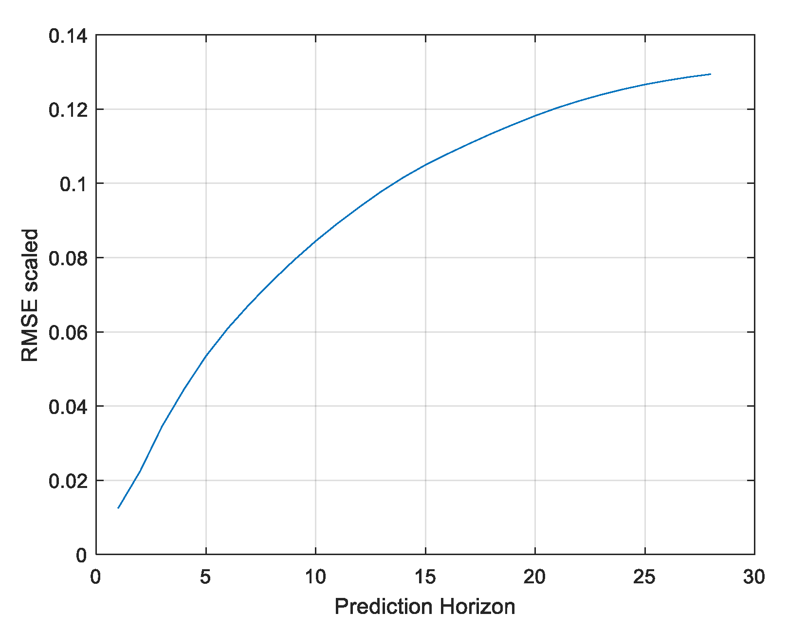
- Prediction Horizon: 28 steps (7 h);
- Number of neuros: ;
- Initial parameter values: OAKM [97];
- Number of training trials: five, best compromise solution;
- Termination criterion: early stopping, with a maximum number of iterations of 50;
- Number of generations: 100;
- Population size: 100;
- Proportion of random emigrants: 0.10;
- Crossover rate: 0.70.
5.3.1. Single Solution
Model 1—Power Demand
- ;
- ;
- OM < 150;
- Minimize .
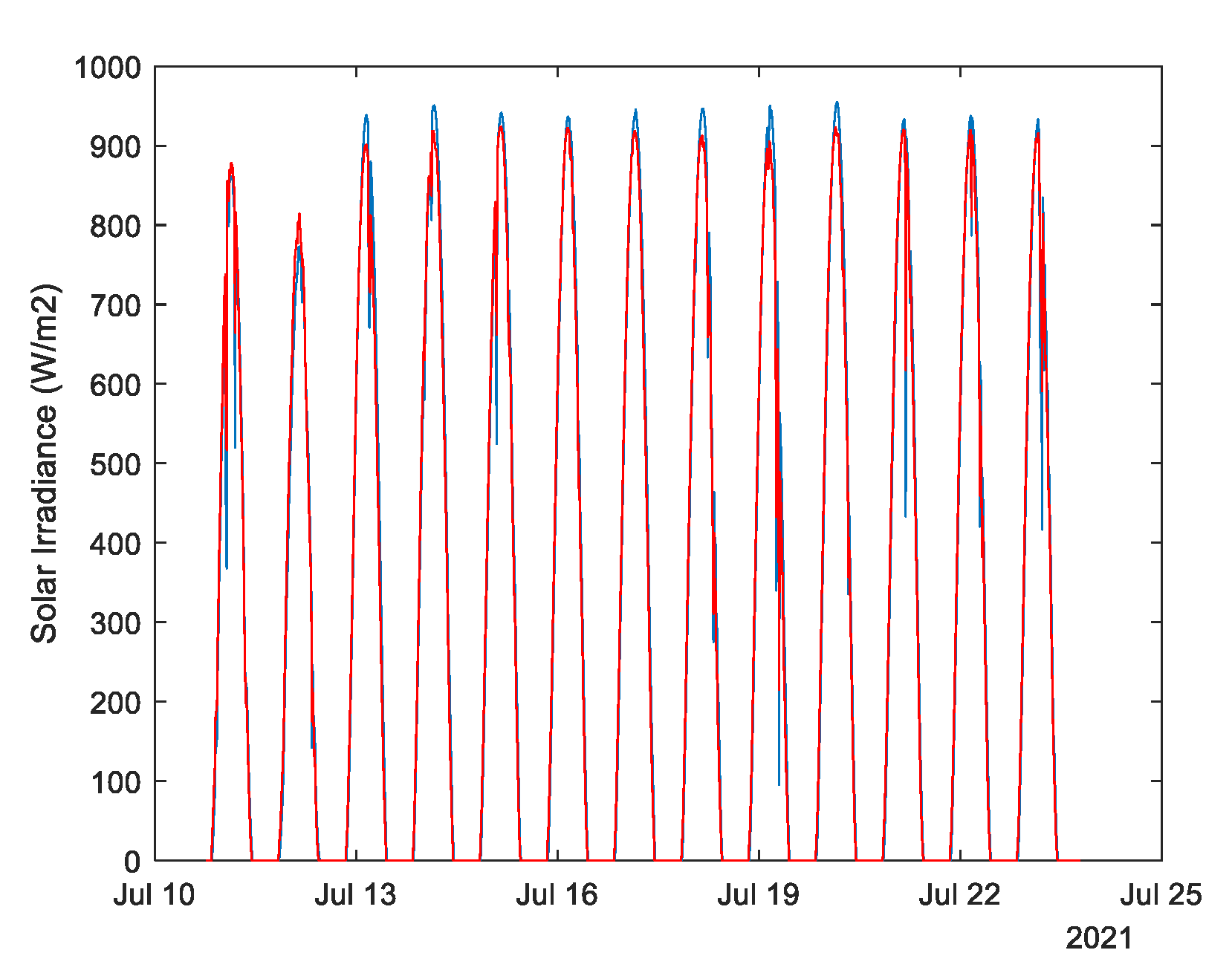
Model 2—Solar Irradiance
- ;
- ;
- OM < 150;
- Minimize .
Model 3—Atmospheric Temperature
- ;
- ;
- OM < 100;
- Minimize .
Model 4—Power Generated
- OM < 100
- Minimize .
5.3.2. Ensemble Averaging
Model 1—Load Demand
Model 2—Solar Irradiance
Model 3—Atmospheric Temperature
Model 4—Power Generated
5.4. Discussion of the Results
Comparison of Results
6. Conclusions
Author Contributions
Funding
Institutional Review Board Statement
Informed Consent Statement
Conflicts of Interest
Abbreviations
| ANN | Artificial Neural Networks |
| ARIMA | Autoregressive Integrated Moving Average |
| BAB | Branch and Bound |
| BPS | Building Performance Simulation |
| CH | Convex Hull |
| DC | Direct Current |
| ELM | Extreme Learning Machines |
| EMS | Energy Management Systems |
| GPR | Ground Penetrating Radar |
| HEMS | Home Energy Management Systems |
| HVAC | Heat Ventilation Air Conditioning |
| HW | Holt-Winters |
| k-NN | k-Nearest Neighbors |
| LR | Linear Regression |
| LSTM | Long Short-Term Memory |
| ML | Machine Learning |
| MOGA | Multi-Objective Genetic Algorithm |
| NAR | Nonlinear Autoregressive |
| NARX | Nonlinear Autoregressive Exogenous |
| NILM | Non-Intrusive Load Monitoring |
| NSGA-II | Nondominated Sorting Genetic Algorithm-II |
| OAKM | Optimal Adaptative K-Means |
| PH | Prediction Horizon |
| PV | Photovoltaics |
| RBF | Radial Basis Function |
| RMSE | Root Mean Square Error |
| RNN | Recursive Neural Networks |
| SPWS | Self-Powered Wireless Sensors |
| SVM | Support Vector Machine |
| SVR | Support Vector Regression |
| WBs | Wibees |
References
- Chou, J.S.; Tran, D.S. Forecasting energy consumption time series using machine learning techniques based on usage patterns of residential householders. Energy 2018, 165, 709–726. [Google Scholar] [CrossRef]
- Lund, H.; Østergaard, P.A.; Connolly, D.; Mathiesen, B.V. Smart energy and smart energy systems. Energy 2017, 137, 556–565. [Google Scholar] [CrossRef]
- Lund, H. Renewable Energy Systems: A Smart Energy Systems Approach to the Choice and Modeling of 100% Renewable Solutions; Academic Press: Cambridge, MA, USA, 2014. [Google Scholar]
- Connolly, D.; Lund, H.; Mathiesen, B.V.; Østergaard, P.A.; Möller, B.; Nielsen, S.; Ridjan, I.; Hvelplund, F.; Sperling, K.; Karnøe, P. Smart Energy Systems: Holistic and Integrated Energy Systems for the Era of 100% Renewable Energy. 2013. Available online: https://vbn.aau.dk/en/publications/smart-energy-systems-holistic-and-integrated-energy-systems-for-t/ (accessed on 14 October 2021).
- Ahmad, T.; Chen, H. A review on machine learning forecasting growth trends and their real-time applications in different energy systems. Sustain. Cities Soc. 2020, 54, 102010. [Google Scholar] [CrossRef]
- Wang, H.Z.; Lei, Z.X.; Zhang, X.; Zhou, B.; Peng, J.C. A review of deep learning for renewable energy forecasting. Energy Convers. Manag. 2019, 198, 111799. [Google Scholar] [CrossRef]
- Liu, H.; Li, Y.; Duan, Z.; Chen, C. A review on multi-objective optimization framework in wind energy forecasting techniques and applications. Energy Convers. Manag. 2020, 224, 113324. [Google Scholar] [CrossRef]
- Sharma, V.; Cortes, A.; Cali, U. Use of Forecasting in Energy Storage Applications: A Review. IEEE Access 2021, 9, 114690–114704. [Google Scholar] [CrossRef]
- Ma, J.; Ma, X.D. A review of forecasting algorithms and energy management strategies for microgrids. Syst. Sci. Control Eng. 2018, 6, 237–248. [Google Scholar] [CrossRef]
- Walther, J.; Weigold, M. A Systematic Review on Predicting and Forecasting the Electrical Energy Consumption in the Manufacturing Industry. Energies 2021, 14, 968. [Google Scholar] [CrossRef]
- Heyets, V.M.; Kyrylenko, O.V.; Basok, B.I.; Baseyev, Y.T. The Energy Strategy: Forecasts and Reality (Review). Sci. Innov. 2020, 16, 3–14. [Google Scholar] [CrossRef]
- Debnath, K.B.; Mourshed, M. Forecasting methods in energy planning models. Renew. Sustain. Energy Rev. 2018, 88, 297–325. [Google Scholar] [CrossRef] [Green Version]
- Wei, N.; Li, C.J.; Peng, X.L.; Zeng, F.H.; Lu, X.Q. Conventional models and artificial intelligence-based models for energy consumption forecasting: A review. J. Pet. Sci. Eng. 2019, 181, 106187. [Google Scholar] [CrossRef]
- Paudel, S.; Elmitri, M.; Couturier, S.; Nguyen, P.H.; Kamphuis, R.; Lacarriere, B.; Le Corre, O. A relevant data selection method for energy consumption prediction of low energy building based on support vector machine. Energy Build. 2017, 138, 240–256. [Google Scholar] [CrossRef]
- Szul, T.; Necka, K.; Mathia, T.G. Neural Methods Comparison for Prediction of Heating Energy Based on Few Hundreds Enhanced Buildings in Four Season’s Climate. Energies 2020, 13, 5453. [Google Scholar] [CrossRef]
- Khan, A.N.; Iqbal, N.; Rizwan, A.; Ahmad, R.; Kim, D.H. An Ensemble Energy Consumption Forecasting Model Based on Spatial-Temporal Clustering Analysis in Residential Buildings. Energies 2021, 14, 3020. [Google Scholar] [CrossRef]
- Aslam, S.; Herodotou, H.; Mohsin, S.M.; Javaid, N.; Ashraf, N.; Aslam, S. A survey on deep learning methods for power load and renewable energy forecasting in smart microgrids. Renew. Sustain. Energy Rev. 2021, 144, 23. [Google Scholar] [CrossRef]
- Singaravel, S.; Suykens, J.; Geyer, P. Deep-learning neural-network architectures and methods: Using component based models in building-design energy prediction. Adv. Eng. Inform. 2018, 38, 81–90. [Google Scholar] [CrossRef]
- Truong, L.M.; Chow, K.H.K.; Luevisadpaibul, R.; Thirunavukkarasu, G.S.; Seyedmahmoudian, M.; Horan, B.; Mekhilef, S.; Stojcevski, A. Accurate Prediction of Hourly Energy Consumption in a Residential Building Based on the Occupancy Rate Using Machine Learning Approaches. Appl. Sci. 2021, 11, 2229. [Google Scholar] [CrossRef]
- Geyer, P.; Singaravel, S. Component-based machine learning for performance prediction in building design. Appl. Energy 2018, 228, 1439–1453. [Google Scholar] [CrossRef]
- Chatfield, C.; Xing, H. The Analysis of Time Series: An Introduction with R; Chapman and hall/CRC: Boca Raton, FL, USA, 2019. [Google Scholar]
- Chatfield, C. The Analysis of Time Series: Theory and Practice; Springer: Berlin/Heidelberg, Germany, 2013. [Google Scholar]
- Divina, F.; Garcia Torres, M.; Goméz Vela, F.A.; Vazquez Noguera, J.L. A comparative study of time series forecasting methods for short term electric energy consumption prediction in smart buildings. Energies 2019, 12, 1934. [Google Scholar] [CrossRef] [Green Version]
- Webby, R.; O’Connor, M. Judgemental and statistical time series forecasting: A review of the literature. Int. J. Forecast. 1996, 12, 91–118. [Google Scholar] [CrossRef]
- Kelleher, J.D.; Mac Namee, B.; D’Arcy, A. Fundamentals of Machine Learning for Predictive Data Analytics: Algorithms, Worked Examples, and Case Studies; MIT Press: Cambridge, MA, USA, 2020. [Google Scholar]
- Deisenroth, M.P.; Faisal, A.A.; Ong, C.S. Mathematics for Machine Learning; Cambridge University Press: Cambridge, UK, 2020. [Google Scholar]
- Shalev-Shwartz, S.; Ben-David, S. Understanding Machine Learning: From Theory to Algorithms; Cambridge University Press: Cambridge, UK, 2014. [Google Scholar]
- Khalil, A.J.; Barhoom, A.M.; Abu-Nasser, B.S.; Musleh, M.M.; Abu-Naser, S.S. Energy Efficiency Prediction using Artificial Neural Network. Int. J. Acad. Pedagog. Res. (IJAPR) 2019, 3, 1–7. [Google Scholar]
- Ahmad, M.W.; Mourshed, M.; Rezgui, Y. Trees vs Neurons: Comparison between random forest and ANN for high-resolution prediction of building energy consumption. Energy Build. 2017, 147, 77–89. [Google Scholar] [CrossRef]
- Li, K.; Xie, X.; Xue, W.; Dai, X.; Chen, X.; Yang, X. A hybrid teaching-learning artificial neural network for building electrical energy consumption prediction. Energy Build. 2018, 174, 323–334. [Google Scholar] [CrossRef]
- Bot, K.; Ruano, A.; Ruano, M.d.G. Short-Term Forecasting Photovoltaic Solar Power for Home Energy Management Systems. Inventions 2021, 6, 12. [Google Scholar] [CrossRef]
- Ruano, A.; Bot, K.; Ruano, M.G. Home Energy Management System in an Algarve residence. First results. In CONTROLO 2020: Proceedings of the 14th APCA International Conference on Automatic Control and Soft Computing; Lecture Notes in Electrical Engineering; Springer Science and Business Media Deutschland GmbH: Bragança, Portugal, 2021; Volume 695, pp. 332–341. [Google Scholar]
- Bot, K.; Ruano, A.; Ruano, M.G. Forecasting Electricity Demand in Households using MOGA-designed Artificial Neural Networks. In Proceedings of the 21st IFAC World Congress, Berlin, Germany, 12–17 July 2020. [Google Scholar]
- Al-Dahidi, S.; Ayadi, O.; Alrbai, M.; Adeeb, J. Ensemble Approach of Optimized Artificial Neural Networks for Solar Photovoltaic Power Prediction. IEEE Access 2019, 7, 81741–81758. [Google Scholar] [CrossRef]
- Zhong, H.; Wang, J.; Jia, H.; Mu, Y.; Lv, S. Vector field-based support vector regression for building energy consumption prediction. Appl. Energy 2019, 242, 403–414. [Google Scholar] [CrossRef]
- Koschwitz, D.; Frisch, J.; Van Treeck, C. Data-driven heating and cooling load predictions for non-residential buildings based on support vector machine regression and NARX Recurrent Neural Network: A comparative study on district scale. Energy 2018, 165, 134–142. [Google Scholar] [CrossRef]
- Li, Y.; Cao, L.; Han, Y.; Shi, Y.; Zhang, Y. Short-Term Electric Load Forecasting with a Hybrid ARIMA, SVR, and IA Methodology; American Society of Civil Engineers: Reston, VA, USA, 2020; pp. 166–175. [Google Scholar]
- Nepal, B.; Yamaha, M.; Yokoe, A.; Yamaji, T. Electricity load forecasting using clustering and ARIMA model for energy management in buildings. Jpn. Archit. Rev. 2020, 3, 62–76. [Google Scholar] [CrossRef] [Green Version]
- Jagait, R.K.; Fekri, M.N.; Grolinger, K.; Mir, S. Load Forecasting Under Concept Drift: Online Ensemble Learning With Recurrent Neural Network and ARIMA. IEEE Access 2021, 9, 98992–99008. [Google Scholar] [CrossRef]
- Kandananond, K. Electricity Demand Forecasting in Buildings Based on ARIMA and ARX Models. In Proceedings of the 8th International Conference on Informatics, Environment, Energy and Applications, Osaka, Japan, 19 March 2019; pp. 268–271. [Google Scholar]
- Wang, Z.; Srinivasan, R.S. A review of artificial intelligence based building energy use prediction: Contrasting the capabilities of single and ensemble prediction models. Renew. Sustain. Energy Rev. 2017, 75, 796–808. [Google Scholar] [CrossRef]
- Tran, D.-H.; Luong, D.-L.; Chou, J.-S. Nature-inspired metaheuristic ensemble model for forecasting energy consumption in residential buildings. Energy 2020, 191, 116552. [Google Scholar] [CrossRef]
- Bontempi, G.; Taieb, S.B.; Le Borgne, Y.-A. Machine Learning Strategies for Time Series Forecasting; Springer: Berlin/Heidelberg, Germany, 2012; pp. 62–77. [Google Scholar]
- Ahmed, N.K.; Atiya, A.F.; Gayar, N.E.; El-Shishiny, H. An empirical comparison of machine learning models for time series forecasting. Econom. Rev. 2010, 29, 594–621. [Google Scholar] [CrossRef]
- Seyedzadeh, S.; Rahimian, F.P.; Glesk, I.; Roper, M. Machine learning for estimation of building energy consumption and performance: A review. Vis. Eng. 2018, 6, 1–20. [Google Scholar] [CrossRef]
- Mosavi, A.; Bahmani, A. Energy Consumption Prediction Using Machine Learning; a Review. Preprints 2019, 2019030131. [Google Scholar] [CrossRef]
- Fathi, S.; Srinivasan, R.; Fenner, A.; Fathi, S. Machine learning applications in urban building energy performance forecasting: A systematic review. Renew. Sustain. Energy Rev. 2020, 133, 110287. [Google Scholar] [CrossRef]
- Mariano-Hernández, D.; Hernández-Callejo, L.; García, F.S.; Duque-Perez, O.; Zorita-Lamadrid, A.L. A Review of Energy Consumption Forecasting in Smart Buildings: Methods, Input Variables, Forecasting Horizon and Metrics. Appl. Sci. 2020, 10, 8323. [Google Scholar] [CrossRef]
- Ahmad, T.; Zhang, H.C. Novel deep supervised ML models with feature selection approach for large-scale utilities and buildings short and medium-term load requirement forecasts. Energy 2020, 209, 16. [Google Scholar] [CrossRef]
- Chou, J.S.; Truong, D.N. Multistep energy consumption forecasting by metaheuristic optimization of time-series analysis and machine learning. Int. J. Energy Res. 2021, 45, 4581–4612. [Google Scholar] [CrossRef]
- Liu, C.; Sun, B.; Zhang, C.H.; Li, F. A hybrid prediction model for residential electricity consumption using holt-winters and extreme learning machine. Appl. Energy 2020, 275, 15. [Google Scholar] [CrossRef]
- Li, X.Y.; Yao, R.M. Modelling heating and cooling energy demand for building stock using a hybrid approach. Energy Build. 2021, 235, 110740. [Google Scholar] [CrossRef]
- Wenninger, S.; Wiethe, C. Benchmarking Energy Quantification Methods to Predict Heating Energy Performance of Residential Buildings in Germany. Bus. Inform. Syst. Eng. 2021, 63, 223–242. [Google Scholar] [CrossRef]
- Ullah, F.U.M.; Ullah, A.; Ul Haq, I.; Rho, S.; Baik, S.W. Short-Term Prediction of Residential Power Energy Consumption via CNN and Multi-Layer Bi-Directional LSTM Networks. IEEE Access 2020, 8, 123369–123380. [Google Scholar] [CrossRef]
- Papadopoulos, S.; Azar, E.; Woon, W.L.; Kontokosta, C.E. Evaluation of tree-based ensemble learning algorithms for building energy performanceestimation. J. Build. Perform. Simul. 2018, 11, 322–332. [Google Scholar] [CrossRef]
- Szul, T.; Tabor, S.; Pancerz, K. Application of the BORUTA Algorithm to Input Data Selection for a Model Based on Rough Set Theory (RST) to Prediction Energy Consumption for Building Heating. Energies 2021, 14, 2779. [Google Scholar] [CrossRef]
- Rahman, A.; Srikumar, V.; Smith, A.D. Predicting electricity consumption for commercial and residential buildings using deep recurrent neural networks. Appl. Energy 2018, 212, 372–385. [Google Scholar] [CrossRef]
- Gong, M.J.; Wang, J.; Bai, Y.; Li, B.; Zhang, L. Heat load prediction of residential buildings based on discrete wavelet transform and tree-based ensemble learning. J. Build. Eng. 2020, 32, 12. [Google Scholar] [CrossRef]
- Bassamzadeh, N.; Ghanem, R. Multiscale stochastic prediction of electricity demand in smart grids using Bayesian networks. Appl. Energy 2017, 193, 369–380. [Google Scholar] [CrossRef]
- Jin, X.; Baker, K.; Christensen, D.; Isley, S. Foresee: A user-centric home energy management system for energy efficiency and demand response. Appl. Energy 2017, 205, 1583–1595. [Google Scholar] [CrossRef]
- Mawson, V.J.; Hughes, B. Coupling simulation with artificial neural networks for the optimisation of HVAC controls in manufacturing environments. Optim. Eng. 2021, 22, 103–119. [Google Scholar] [CrossRef]
- Movahedi, A.; Derrible, S. Interrelationships between electricity, gas, and water consumption in large-scale buildings. J. Ind. Ecol. 2021, 25, 932–947. [Google Scholar] [CrossRef]
- Kaur, J.; Bala, A. Predicting power for home appliances based on climatic conditions. Int. J. Energy Sect. Manag. 2019, 13, 610–629. [Google Scholar] [CrossRef]
- Shen, M.; Lu, Y.J.; Wei, K.H.; Cui, Q.B. Prediction of household electricity consumption and effectiveness of concerted intervention strategies based on occupant behaviour and personality traits. Renew. Sustain. Energy Rev. 2020, 127, 109839. [Google Scholar] [CrossRef]
- Liu, S.; Zeng, A.; Lau, K.; Ren, C.; Chan, P.W.; Ng, E. Predicting long-term monthly electricity demand under future climatic and socioeconomic changes using data-driven methods: A case study of Hong Kong. Sustain. Cities Soc. 2021, 70, 102936. [Google Scholar] [CrossRef]
- Honda. Honda Smart Home US. Available online: https://www.hondasmarthome.com (accessed on 14 October 2019).
- Leitao, J.; Fonseca, C.M.; Gil, P.; Ribeiro, B.; Cardoso, A. A Compressive Receding Horizon Approach for Smart Home Energy Management. IEEE Access 2021, 9, 100407–100435. [Google Scholar] [CrossRef]
- Huang, H.T.; Xu, H.; Cai, Y.H.; Khalid, R.S.; Yu, H. Distributed Machine Learning on Smart-Gateway Network toward Real-Time Smart-Grid Energy Management with Behavior Cognition. ACM Transact. Des. Automat. Electron. Syst. 2018, 23, 26. [Google Scholar] [CrossRef]
- Aurangzeb, K. Short Term Power Load Forecasting using Machine Learning Models for energy management in a smart community. In Proceedings of the 2019 International Conference on Computer and Information Sciences (ICCIS), Sakaka, Saudi Arabia, 3–4 April 2019; pp. 1–6. [Google Scholar]
- Zaouali, K.; Rekik, R.; Bouallegue, R. Deep learning forecasting based on auto-lstm model for home solar power systems. In Proceedings of the 2018 IEEE 20th International Conference on High Performance Computing and Communications, Exeter, UK, 28–30 June 2018; pp. 235–242. [Google Scholar]
- Shakir, M.; Biletskiy, Y. Forecasting and optimisation for microgrid in home energy management systems. IET Gener. Transm. Distrib. 2020, 14, 3458–3468. [Google Scholar] [CrossRef]
- Ahmadiahangar, R.; Häring, T.; Rosin, A.; Korõtko, T.; Martins, J. Residential load forecasting for flexibility prediction using machine learning-based regression model. In Proceedings of the 2019 IEEE International Conference on Environment and Electrical Engineering and 2019 IEEE Industrial and Commercial Power Systems Europe (EEEIC / I&CPS Europe), Genova, Italy, 11–14 June 2019; pp. 1–4. [Google Scholar]
- Rajasekaran, R.G.; Manikandaraj, S.; Kamaleshwar, R. Implementation of machine learning algorithm for predicting user behavior and smart energy management. In Proceedings of the 2017 International Conference on Data Management, Analytics and Innovation (ICDMAI), Pune, India, 24–26 February 2017; pp. 24–30. [Google Scholar]
- Koltsaklis, N.; Panapakidis, I.P.; Pozo, D.; Christoforidis, G.C. A Prosumer Model Based on Smart Home Energy Management and Forecasting Techniques. Energies 2021, 14, 1724. [Google Scholar] [CrossRef]
- Fan, L.; Li, J.; Zhang, X.-P. Load prediction methods using machine learning for home energy management systems based on human behavior patterns recognition. CSEE J. Power Energy Syst. 2020, 6, 563–571. [Google Scholar]
- Li, W.; Logenthiran, T.; Phan, V.-T.; Woo, W.L. Implemented IoT-based self-learning home management system (SHMS) for Singapore. IEEE Internet Things J. 2018, 5, 2212–2219. [Google Scholar] [CrossRef]
- Khan, M.; Seo, J.; Kim, D. Towards Energy Efficient Home Automation: A Deep Learning Approach. Sensors 2020, 20, 7187. [Google Scholar] [CrossRef] [PubMed]
- Arens, S.; Derendorf, K.; Schuldt, F.; Maydell, K.V.; Agert, C. Effect of EV movement schedule and machine learning-based load forecasting on electricity cost of a single household. Energies 2018, 11, 2913. [Google Scholar] [CrossRef] [Green Version]
- Prophet. Prophet, Forecasting at Scale. Available online: https://facebook.github.io/prophet/ (accessed on 2 November 2021).
- AtsPy. AtsPy: Automated Time Series Models in Python. Available online: https://github.com/firmai/atspy (accessed on 2 November 2021).
- Yuan, X.M.; Han, P.; Duan, Y.; Alden, R.E.; Rallabandi, V.; Ionel, D.M. Residential Electrical Load Monitoring and Modeling—State of the Art and Future Trends for Smart Homes and Grids. Electr. Power Compon. Syst. 2020, 48, 1125–1143. [Google Scholar] [CrossRef]
- Laouali, I.H.; Qassemi, H.; Marzouq, M.; Ruano, A.; Bennani, S.D.; El Fadili, H. A Survey on Computational Intelligence Techniques For Non Intrusive Load Monitoring. In Proceedings of the 2020 IEEE 2nd International Conference on Electronics, Control, Optimization and Computer Science (ICECOCS), Kenitra, Morocco, 2–3 December 2020; pp. 1–6. [Google Scholar]
- Ruano, A.; Hernandez, A.; Ureña, J.; Ruano, M.; Garcia, J. NILM Techniques for Intelligent Home Energy Management and Ambient Assisted Living: A Review. Energies 2019, 12, 2203. [Google Scholar] [CrossRef] [Green Version]
- Hosseini, S.S.; Agbossou, K.; Kelouwani, S.; Cardenas, A. Non-intrusive load monitoring through home energy management systems: A comprehensive review. Renew. Sustain. Energy Rev. 2017, 79, 1266–1274. [Google Scholar] [CrossRef]
- Zeifman, M.; Roth, K. Nonintrusive appliance load monitoring: Review and outlook. IEEE Trans. Consum. Electron. 2011, 57, 76–84. [Google Scholar] [CrossRef]
- Lemes, D.A.M.; Cabral, T.W.; Fraidenraich, G.; Meloni, L.G.P.; De Lima, E.R.; Neto, F.B. Load Disaggregation Based on Time Window for HEMS Application. IEEE Access 2021, 9, 70746–70757. [Google Scholar] [CrossRef]
- Lin, Y.-H.; Tsai, M.-S. An advanced home energy management system facilitated by nonintrusive load monitoring with automated multiobjective power scheduling. IEEE Trans. Smart Grid 2015, 6, 1839–1851. [Google Scholar] [CrossRef]
- Zhai, S.; Wang, Z.; Yan, X.; He, G. Appliance flexibility analysis considering user behavior in home energy management system using smart plugs. IEEE Trans. Ind. Electron. 2018, 66, 1391–1401. [Google Scholar] [CrossRef]
- Khosravani, H.R.; Ruano, A.E.; Ferreira, P.M. A convex hull-based data selection method for data driven models. Appl. Soft Comput. 2016, 47, 515–533. [Google Scholar] [CrossRef]
- Ruano, A.E.; Pesteh, S.; Silva, S.; Duarte, H.; Mestre, G.; Ferreira, P.M.; Khosravani, H.R.; Horta, R. The IMBPC HVAC system: A complete MBPC solution for existing HVAC systems. Energy Build. 2016, 120, 145–158. [Google Scholar] [CrossRef]
- Siemens Smart Infrastructure. Energy Intelligence—Tapping the Potential of a Smart Energy World; Siemens Switzerland Ltd.: Zug, Switzerland, 2020. [Google Scholar]
- Gordillo-Orquera, R.; Lopez-Ramos, L.M.; Muñoz-Romero, S.; Iglesias-Casarrubios, P.; Arcos-Avilés, D.; Marques, A.G.; Rojo-Álvarez, J.L. Analyzing and Forecasting Electrical Load Consumption in Healthcare Buildings. Energies 2018, 11, 493. [Google Scholar] [CrossRef] [Green Version]
- Ferreira, P.; Ruano, A. Evolutionary Multiobjective Neural Network Models Identification: Evolving Task-Optimised Models. In New Advances in Intelligent Signal Processing; Ruano, A., Várkonyi-Kóczy, A., Eds.; Springer: Berlin/Heidelberg, Germany, 2011; Volume 372, pp. 21–53. [Google Scholar]
- Levenberg, K. A method for the solution of certain problems in least squares. Q. Appl. Math. 1944, 2, 164–168. [Google Scholar] [CrossRef] [Green Version]
- Marquardt, D. An algorithm for least-squares estimation of nonlinear parameters. SIAM J. Appl. Math. 1963, 11, 431–441. [Google Scholar] [CrossRef]
- Ruano, A.E.B.; Jones, D.I.; Fleming, P.J. A New Formulation of the Learning Problem for a Neural Network Controller. In Proceedings of the 30th IEEE Conference on Decision and Control, Brighton, UK, 11–13 December 1991; pp. 865–866. [Google Scholar]
- Chinrunngrueng, C.; Séquin, C.H. Optimal adaptive k-means algorithm with dynamic adjustment of learning rate. IEEE Trans. Neural Netw. 1995, 6, 157–169. [Google Scholar] [CrossRef] [PubMed]
- Lineros, M.L.; Luna, A.M.; Ferreira, P.M.; Ruano, A.E. Optimized Design of Neural Networks for a River Water Level Prediction System. Sensors 2021, 21, 6504. [Google Scholar] [CrossRef] [PubMed]
- Sharp NU-AK PV Panels. Available online: https://www.sharp.co.uk/cps/rde/xchg/gb/hs.xsl/-/html/product-details-solar-modules-2189.htm?product=NUAK300B (accessed on 14 October 2021).
- Kostal Plenticore Plus Inverter. Available online: https://www.kostal-solar-electric.com/en-gb/products/hybrid-inverters/plenticore-plus (accessed on 14 October 2021).
- BYD Battery Box HV. Available online: https://www.eft-systems.de/en/The%20B-BOX/product/Battery%20Box%20HV/3 (accessed on 14 October 2021).
- Mestre, G.; Ruano, A.; Duarte, H.; Silva, S.; Khosravani, H.; Pesteh, S.; Ferreira, P.; Horta, R. An Intelligent Weather Station. Sensors 2015, 15, 31005–31022. [Google Scholar] [CrossRef]
- TP-Link WiFi Smart Plugs. Available online: https://www.tp-link.com/pt/home-networking/smart-plug/hs100/ (accessed on 14 October 2021).
- Ruano, A.; Silva, S.; Duarte, H.; Ferreira, P.M. Wireless Sensors and IoT Platform for Intelligent HVAC Control. Appl. Sci. 2018, 8, 370. [Google Scholar] [CrossRef] [Green Version]
- Carlo Gavazzi EM340. Available online: https://www.carlogavazzi.co.uk/blog/carlo-gavazzi-energy-solutions/em340-utilises-touchscreen-technology (accessed on 14 October 2021).
- Wibeee Consumption Analyzers. Available online: http://circutor.com/en/products/measurement-and-control/fixed-power-analyzers/consumption-analyzers (accessed on 14 October 2021).
- Ferreira, P.M.; Ruano, A.E.; Pestana, R.; Koczy, L.T. Evolving RBF predictive models to forecast the Portuguese electricity consumption. IFAC Proc. 2009, 42, 414–419. [Google Scholar] [CrossRef]
- Ferreira, P.M.; Pestana, R.; Ruano, A.E. Improving the Identification of RBF Predictive Models to Forecast the Portuguese Electricity Consumption. IFAC Proc. 2010, 1, 208–213. [Google Scholar] [CrossRef]
- Bot, K.; Laouali, I.; Ruano, A.; Ruano, M.d.G. Home Energy Management Systems with Branch-and-Bound Model-Based Predictive Control Techniques. Energies 2021, 14, 5852. [Google Scholar] [CrossRef]
- Ruano, A.; Bot, K.; Ruano, M.d.G. The Impact of Occupants in Thermal Comfort and Energy Efficiency in Buildings. In Occupant Behaviour in Buildings: Advances and Challenges, Bentham Science: Sharjah. United Arab Emirates 2021, 6, 101–137. [Google Scholar]
- Ferreira, P.M.; Ruano, A.E.; Pestana, R. Towards Online Operation of a RBF Neural Network Model to Forecast the Portuguese Electricity Consumption. In Proceedings of the 2011 IEEE 7th International Symposium on Intelligent Signal Processing (WISP), Floriana, Malta, 19–21 September 2021. [Google Scholar]
- Ferreira, P.M.; Cuambe, I.D.; Ruano, A.E.; Pestana, R. Forecasting the Portuguese Electricity Consumption using Least-Squares Support Vector Machines. IFAC Proc. 2013, 3, 411–416. [Google Scholar] [CrossRef]
- Zhang, X.M.; Grolinger, K.; Capretz, M.A.M.; Seewald, L. Forecasting Residential Energy Consumption: Single Household Perspective. In Proceedings of the 17th IEEE International Conference on Machine Learning and Applications (IEEE ICMLA), Orlando, FL, USA, 17–20 December 2018; pp. 110–117. [Google Scholar]
- Wen, L.; Zhou, K.; Yang, S. Load demand forecasting of residential buildings using a deep learning model. Electr. Power Syst. Res. 2020, 179, 106073. [Google Scholar] [CrossRef]
- Pecan Street Inc. Dataport. Available online: https://www.pecanstreet.org/dataport/ (accessed on 14 October 2021).
- Rana, M.; Rahman, A. Multiple steps ahead solar photovoltaic power forecasting based on univariate machine learning models and data re-sampling. Sustain. Energy Grids Netw. 2020, 21, 100286. [Google Scholar] [CrossRef]
- Hossain, M.S.; Mahmood, H. Short-Term Photovoltaic Power Forecasting Using an LSTM Neural Network and Synthetic Weather Forecast. IEEE Access 2020, 8, 172524–172533. [Google Scholar] [CrossRef]
- Wang, K.; Qi, X.; Liu, H. A comparison of day-ahead photovoltaic power forecasting models based on deep learning neural network. Appl. Energy 2019, 251, 113315. [Google Scholar] [CrossRef]
- Li, G.; Xie, S.; Wang, B.; Xin, J.; Li, Y.; Du, S. Photovoltaic Power Forecasting with a Hybrid Deep Learning Approach. IEEE Access 2020, 8, 175871–175880. [Google Scholar] [CrossRef]


| Day of the Week | Regular Day | Holiday | Special |
|---|---|---|---|
| Monday | 0.05 | 0.40 | 0.70 |
| Tuesday | 0.10 | 0.80 | |
| Wednesday | 0.15 | 0.50 | |
| Thursday | 0.20 | 1.00 | |
| Friday | 0.25 | 0.60 | 0.90 |
| Saturday | 0.30 | 0.30 | |
| Sunday | 0.35 | 0.35 |
| Execution | ||||
|---|---|---|---|---|
| 1st | 0.14 | 0.12 | 0.12 | 4.81 |
| 2nd | 0.15 | 0.12 | 0.12 | 4.79 |
| Execution | ||||
|---|---|---|---|---|
| 1st | 0.11 | 0.08 | 0.08 | 2.58 |
| 2nd | 0.11 | 0.08 | 0.08 | 2.58 |
| Execution | ||||
|---|---|---|---|---|
| 1st | 0.02 | 0.02 | 0.02 | 2.72 |
| 2nd | 0.02 | 0.02 | 0.02 | 2.70 |
| Execution | ||||
|---|---|---|---|---|
| 1st | 0.05 | 0.04 | 0.05 | 1.69 |
| 2nd | 0.06 | 0.04 | 0.05 | 1.67 |
| 4.14 | 4.61 | 5.14 | 1.00 | |
| 4.16 | 4.61 | 5.10 | 0.94 | |
| 4.17 | 4.62 | 5.10 | 0.93 | |
| 4.04 | 4.67 | 5.53 | 1.49 | |
| 4.04 | 4.67 | 5.53 | 1.49 | |
| 4.18 | 4.65 | 5.17 | 0.99 |
| 2.27 | 2.46 | 2.66 | 0.35 | |
| 2.26 | 2.47 | 2.70 | 0.44 | |
| 2.25 | 2.48 | 2.72 | 0.47 | |
| 2.15 | 2.55 | 3.07 | 0.92 | |
| 2.25 | 2.53 | 2.84 | 0.59 | |
| 2.28 | 2.54 | 2.80 | 0.52 |
| 2.38 | 2.59 | 2.84 | 0.46 | |
| 2.40 | 2.58 | 2.78 | 0.38 | |
| 2.42 | 2.59 | 2.78 | 0.36 | |
| 2.35 | 2.62 | 2.92 | 0.57 | |
| 2.35 | 2.59 | 2.89 | 0.54 | |
| 2.38 | 2.59 | 2.85 | 0.47 |
| 1.19 | 1.44 | 1.75 | 0.56 | |
| 1.14 | 1.41 | 1.73 | 0.59 | |
| 1.09 | 1.38 | 1.74 | 0.65 | |
| 1.24 | 1.65 | 2.16 | 0.92 | |
| 1.18 | 1.56 | 2.05 | 0.87 | |
| 1.15 | 1.51 | 2.08 | 0.87 |
Publisher’s Note: MDPI stays neutral with regard to jurisdictional claims in published maps and institutional affiliations. |
© 2021 by the authors. Licensee MDPI, Basel, Switzerland. This article is an open access article distributed under the terms and conditions of the Creative Commons Attribution (CC BY) license (https://creativecommons.org/licenses/by/4.0/).
Share and Cite
Bot, K.; Santos, S.; Laouali, I.; Ruano, A.; Ruano, M.d.G. Design of Ensemble Forecasting Models for Home Energy Management Systems. Energies 2021, 14, 7664. https://doi.org/10.3390/en14227664
Bot K, Santos S, Laouali I, Ruano A, Ruano MdG. Design of Ensemble Forecasting Models for Home Energy Management Systems. Energies. 2021; 14(22):7664. https://doi.org/10.3390/en14227664
Chicago/Turabian StyleBot, Karol, Samira Santos, Inoussa Laouali, Antonio Ruano, and Maria da Graça Ruano. 2021. "Design of Ensemble Forecasting Models for Home Energy Management Systems" Energies 14, no. 22: 7664. https://doi.org/10.3390/en14227664