Decarbonizing Local Mobility and Greenhouse Agriculture through Residential Building Energy Upgrades: A Case Study for Québec

Abstract

Electrification is an efficient way to decarbonize by replacing fossil fuels with low-emission power. In addition, energy efficiency measures can reduce consumption, making it easier to shift to a zero-carbon society. In Québec, upgrades to aging buildings that employ electric resistance heating offer a unique opportunity to free up large amounts of hydroelectricity that can serve to decarbonize heating in other buildings. However, another source of energy would be needed to electrify mobility because efficiency measures free up small amounts of electricity in summer compared to winter. This study reveals how building efficiency measures combined with solar electricity generation provide an energy profile that matches the requirements for decarbonizing both mobility and heating. The TRNSYS software was used to simulate the annual energy performance of an existing house and retrofitted/rebuilt low-energy houses equipped with a photovoltaic (PV) roof in Montreal, Québec, Canada (45.5° N). The electricity that is made available by upgrading the houses is mainly considered for powering battery and fuel cell electric vehicles (BEVs and FCEVs) and electrifying heating in greenhouses. The results indicate that retrofitting 16% or rebuilding 12% of single-detached homes in Québec can provide enough electricity to decarbonize heating energy use in existing greenhouses and to operate the new greenhouses required for growing all fresh vegetables locally. If all the single-detached houses that employ electric resistance heating are upgraded, 33.4 and 21.8 TWh year⁻¹ of electricity would be available for decarbonization, equivalent to a 19% and 12% increase of the province’s electricity supply for the retrofitted or rebuilt houses, respectively. This is enough energy to convert 83–100% of personal vehicles to BEVs or 35–56% to FCEVs. Decarbonization using the electricity that is made available by upgrading to low-energy solar houses could reduce the province’s greenhouse gas (GHG) emissions by approximately 32% (26.5 MtCO_2eq). The time required for the initial embodied GHG emissions to surpass the emissions avoided by electrification ranges from 3.4 to 11.2 years. Building energy efficiency retrofits/rebuilds combined with photovoltaics is a promising approach for Québec to maximize the decarbonization potential of its existing energy resources while providing local energy and food security.

1. Introduction

As humans strive to reduce environmental degradation, fossil fuels will increasingly be substituted with low-emission energy sources such as renewable electricity. The sectors that require decarbonization the most are transportation, which represents 45% of Québec’s greenhouse gas (GHG) emissions, and the energy used to heat buildings, greenhouses, and industrial processes [1]. The transportation sector is particularly in need of transformation due to high personal vehicle ownership, long commutes, large travel distances for goods produced elsewhere, and inefficient internal combustion engines that produce harmful pollution such as particulate matter directly in the city.

For many applications, the preferred decarbonization pathway is electrification because of the higher efficiency of electrical devices. For instance, electric motors are around 90% efficient compared to 20% for internal combustion engines [2], and heat pumps can achieve heating at least three times more efficiently than electric resistance heating [3]. Electrification always reduces emissions when a low-emission electricity supply is employed. However, electrification increases electricity demand. A study for Canada estimates that electricity consumption will need to be doubled by 2050 [4]. One of the greatest challenges of the energy transition will be to identify and implement the most effective solutions for supplying the energy required for decarbonization.

Typically, the new power supply would be provided using one or a mix of renewable energy resources such as wind, solar, and to a lesser extent biomass or nuclear, as a low-emission (i.e., emits low amounts of pollution such as GHGs and particulate matter) non-renewable energy resource. An alternative option that does not require new power generation infrastructure is to implement energy efficiency measures to reduce electricity demand from the utility, thereby freeing up generation capacity for other applications. The decarbonization potential of this saved energy depends on the electric utility’s power mix and the performance of the improved energy systems. For instance, reducing electricity use in Québec, whose grid is almost entirely hydropower, would free up low- emission power generation capacity that can be used to decarbonize other sectors such as mobility and heating (can be seen as indirect decarbonization). In contrast, energy efficiency measures applied in Alberta, whose electric grid is mostly powered by fossil fuels, would directly reduce emissions (direct decarbonization) but does not provide low- emission power for decarbonization elsewhere. The annual profile of freed-up electricity depends on when and how much a given efficiency measure reduces energy use. For example, switching from electric resistance heating to a heat pump would free up energy mainly in the winter, which is ideal for electrifying and decarbonizing the heating energy used in other buildings. Upgrading to more energy-efficient appliances would free up a more or less equal amount of energy throughout the year and this matches the requirements for electrifying mobility, which also has a near-constant demand for energy year-round.

In Québec, the grid consists of nearly 96% hydroelectricity [5] and almost 61% of residential buildings are heated with electrical resistance heating [6]. These two conditions provide a unique opportunity to take advantage of energy efficiency and free up a power that the utility can redirect elsewhere, particularly in the winter as heating makes up a large portion of building energy use. Potentially large amounts of electricity can be freed up by implementing building energy upgrades, most notably by switching from electric resistance to heat pumps [7]. This freed-up electricity can be valuable for decarbonizing heating in other buildings, for instance, by converting natural gas heating to electric heat pumps. This would result in the more effective use of the province’s existing low-emission power generation infrastructure, particularly during the winter, when peak demand occurs and new generation capacity is in short supply. Every year, many buildings will be retrofitted or rebuilt due to aging or the owner’s personal choice and there is an opportunity for energy efficiency upgrades to play a significant role as a decarbonization solution.

The electricity that is made available from building upgrades could be prioritized for decarbonizing mobility and heating because they represent the largest contributors to GHG emissions and are amongst the most challenging for the utility to electrify due to issues related to the peak power supply. Greenhouses consume significant amounts of fossil fuels for heating and this trend will accelerate as the Québec government plans to increase local food production by doubling the province’s greenhouse crop production area by 2025 [8]. Most of the existing greenhouses are heated with natural gas and the new ones will likely follow the same path for economic reasons. As a consequence, emissions will increase unless low-emission energy source(s) are employed for their operation. Options for heating decarbonization include electrification, solar energy [9,10,11], and the use of biomass boilers/gasifiers for heating [12] or combined heat and power for lighting and heating [13], including using crop waste as an energy source [14]. A challenge with electrifying heating in greenhouses is their large thermal energy consumption and power demand during peak periods, often making the use of heat pumps cost-prohibitive. If greenhouses would switch from natural gas to electric resistance heating, the impact on grid peak power demand can be considerable, particularly for Québec, where peak demand occurs in winter due to the widespread use of electric heating. Hydro-Québec now offers incentives for demand-side management and estimates that a new power supply during peak periods will be needed by 2025 [15,16]. Therefore, redirecting the electricity that is made available from building energy upgrades to secure low-emission greenhouse operation is prioritized in this work.

For high-latitude locations, building energy efficiency frees up significantly less electricity in the summer (and shoulder seasons) because the potential energy reductions during these periods (e.g., achieved mainly by more efficient appliances, lighting, and water heating) are small compared to the potential energy savings from space heating. Since electrifying mobility requires a near-constant annual supply of low-emission electricity as vehicles travel approximately the same distance throughout the year, the potential decarbonization that can be achieved from building upgrades is limited by the relatively low amount of electricity that can be freed up by energy efficiency measures in summer. Therefore, to address the priority objective of decarbonizing the mobility sector, another source of energy (concentrated in the summer) would be needed to complement the energy that is freed up due to efficiency measures (concentrated in the winter).

This study investigates the combination of energy efficiency and solar electricity generation as a promising way to increase the potential for decarbonizing mobility in the summer. During this period, the higher solar energy generation complements the low amount of electricity that is freed up by efficiency measures, and the opposite occurs in the winter. The combo of energy that is made available by implementing energy efficiency measures and solar energy generation might provide a greater potential for electrifying constant loads (such as required for electric vehicles (EVs) and domestic hot water (DHW) heating) than would be possible if they were implemented separately. Various studies have been conducted to quantify the potential energy savings from efficiency measures [17,18], energy generation from on-site solar energy conversion technologies [19,20], and their associated cost and emissions analysis [21,22,23]. However, from an extensive literature review, there are not any studies that evaluate how the energy supplied from building energy upgrades can serve for decarbonization purposes. More specifically, how can upgrading aging residential buildings to low-energy solar buildings increase the potential for decarbonizing mobility and heating?

In particular, this study analyzes existing single-detached residential houses that are retrofitted/rebuilt and equipped with photovoltaic (PV) roofs in Montreal, Québec, Canada (45.5° N, mid-latitude, 4457 heating degree-days). Figure 1 illustrates how upgrading existing buildings can make electricity available to the building itself and/or the utility that redirects it for decarbonization purposes. The existing building can be retrofitted (i.e., the structure is kept and energy savings achieved by improving the envelope design and heating, ventilation, and air conditioning system, etc.) or demolished and rebuilt to a low-energy solar building. The energy generated from PV may be partly consumed by the building (e.g., self-consumed for its operation, to power the occupant’s EV(s), or to operate a greenhouse located on the land lot) while any excess is exported to the utility who redirects it for decarbonization applications elsewhere. The sum of the produced solar power and the savings due to energy efficiency provides the utility with a low-emission power supply that can help to achieve society’s decarbonization targets. In particular, this study considers the potential use of the electricity that is made available from the building upgrade for powering battery and fuel cell personal EVs and for electrifying the heating energy used in buildings, including for greenhouse crop production.

2. Energy and Emissions Analysis

The energy consumption of a typical house is compared to two upgrade scenarios: one where the existing single-detached house is retrofitted (efficiency measures applied while keeping the main structure) and the other where it is demolished and rebuilt. The upgraded houses generate electricity on-site with a building-applied PV roof for the retrofit house and a more resource-efficient building-integrated PV roof for the new construction. The first step of the analysis is to quantify the total amount of electricity that can be made available by upgrading a single-detached house or “upgrade energy”, which includes contributions from solar electricity generation plus the electricity that is freed up by implementing energy efficiency measures. Then, the amount of mobility and heating (including for greenhouses) that can be electrified using the upgrade energy will be determined based on various scenarios that are described in detail in Section 2.4. This analysis requires energy models for each house and the greenhouse. Annual energy simulations will be performed to quantify their energy performance and the associated GHG emissions.

2.1. House Characteristics

Two main scenarios are compared for upgrading an existing house. The first is to retrofit the existing house and the second is to rebuild it. For the rebuild option, the house geometry changes, whereby two houses are built on the same land lot to provide results that reflect the growing trend of densification (reduces inhabitant land and energy requirements). The existing and retrofitted single-story houses have a basement and a main living floor above it, with a slab-on-grade garage connected to it (Figure 2a). The new houses are designed to have the same living area (typically excluding basement and garage) as their existing counterparts (140 m²). Although the footprint of residential buildings in Canada has increased by approximately 20% in the last 30 years [1], future trends may be different as compact cities and environmentally friendly lifestyles are favored. For a balanced prediction given these uncertainties, the newly built houses were specified to have the same living area as its existing counterpart which also allows a fairer comparison of their energy performance. To build two houses on the same land lot (∼850 m²) while maximizing available outdoor space, the new homes will have two stories (Figure 2b). Similarly, the new houses will have an attached garage and a basement. The houses are equipped with heating and cooling and the upgraded houses also have energy recovery ventilation.

The more compact design of the rebuilt houses causes them to have a smaller area for PV production compared to the retrofitted house. Both houses are upgraded to the same level of energy efficiency. The applied energy efficiency measures are related to the space and DHW heating, the building envelope (insulation, windows and movable shades), and ventilation. The south-facing roof of the upgraded houses is equipped with a PV system consisting of monocrystalline PV modules and an inverter. The roof surface area covered by PV is 97.7 m² and 46.1 m², producing 20.7 kW and 9.8 kW of peak electricity for the retrofitted and rebuilt houses, respectively. Additional details for the modeled houses can be found in a previous study by Bambara, Athienitis and Eicker [7].

2.2. Greenhouse Characteristics

The modeled greenhouse is a typical single pane glass greenhouse with artificial lighting used for the consistent production of crops year-round. Heating and ventilation are used to control inside humidity and temperature. Thermal shading screens reduce night heat loss and are also used to control sunlight levels. The modeled greenhouse has an equal length and width of 30.5 m, a height of 3.7 m, and a total area of 929 m² (10,000 sqft). More of the details for the greenhouse can be found in a previous study by Bambara and Athienitis [24].

2.3. Energy Modeling and Simulation

The TRNSYS 17.2 software (Thermal Energy System Specialists, LLC, Madison, WI, USA) was selected for the transient simulation of the house and greenhouse climate [25]. A majority of the population and thus house upgrades would be located between Montreal and Québec City. Since these two locations have similar weather, the simulations will be performed for Montreal.

House energy performance

Table 1. Energy performance of the existing, retrofitted, and rebuilt houses (values are based on 140 m² of living area for all three houses).

Month	Average Exterior Air Temperature (°C)	Existing House Total Energy Use (kWh m−2)	Retrofit		Rebuild
			Total Energy Use (kWh m−2)	Solar Electricity Generation (kWh m−2)	Total Energy Use (kWh m−2)	Solar Electricity Generation (kWh m−2)
January	−10.1	29	11	14	10	7
February	−8.8	24	8	18	7	9
March	−2.2	19	5	24	5	11
April	5.8	11	4	21	3	10
May	13.3	7	3	24	3	11
June	17.9	6	3	23	3	11
July	21.1	6	4	24	4	11
August	19.6	5	4	21	4	10
September	14.6	6	3	21	3	10
October	8.5	9	3	16	3	7
November	1.9	15	4	8	4	4
December	−6.8	26	8	10	7	5
Total	6.3	161	60	224	56	106

provides the monthly energy consumption and production for the existing, retrofitted, and rebuilt houses. These monthly values were obtained by summing hourly simulation output data. The annual energy consumption of the existing house is sufficiently close to the value reported by [26] for single-detached houses.

Greenhouse energy consumption

The greenhouse energy model developed by Bambara and Athienitis [24] was used for this study. The simulations were performed for Ottawa and assumed to be adequate for representing conditions in Montreal, which is nearby and has sufficiently similar weather. The energy consumed for heating and lighting is in good agreement with those reported for Québec greenhouses with a thermal screen [27,28]. Since approximately 98% of Canadian greenhouse production is dedicated to growing fruiting crops such as tomatoes [29], the daily lighting integral was increased to 21 mol m⁻² d⁻¹ to reflect their growing needs [28]. The heating energy is provided by burning natural gas inside the greenhouse. Other energy such as pumping, air circulation fans, etc. is taken as 34 kWh m⁻² and ventilation fan power is calculated using 4.7 W m⁻³ h⁻¹ [30].

Table 2. Greenhouse energy consumption and peak demand.

Month	Heating Energy (kWh m−2)	Lighting Energy (kWh m−2)	Other Energy (kWh m−2)	Total Energy (kWh m−2)
January	125	43	2	170
February	120	14	2	137
March	99	5	2	106
April	55	4	2	62
May	28	3	3	33
June	13	1	4	18
July	6	2	5	12
August	9	4	4	17
September	22	6	3	31
October	45	23	2	70
November	63	48	2	113
December	100	53	2	156
Total energy (kWh m−2 year−1)	684	206	34	925
Peak power demand (kW m−2)	0.28	0.22	0.003	0.50

provides the peak winter demand and monthly energy consumption that was obtained by summing hourly simulation output data.

2.4. Energy Analysis

The energy that is made available by upgrading an existing building to a low-energy solar building is saved primarily by the utility and a portion may be self-consumed on-site (Figure 1). For the scenarios considered in this study, it is assumed that all of the electricity that is made available from building upgrades (sum of contributions from solar and energy efficiency) is saved by the utility that redirects it for mobility and heating decarbonization applications.

The present analysis considers single-detached houses but the methodology could be expanded to cover other residential buildings such as attached houses and apartments. In addition, only houses that employ electric resistance heating were considered because they are the most commonly used heating systems in Québec and their low efficiency provides significant potential for freeing up electricity from the applied energy efficiency measures.

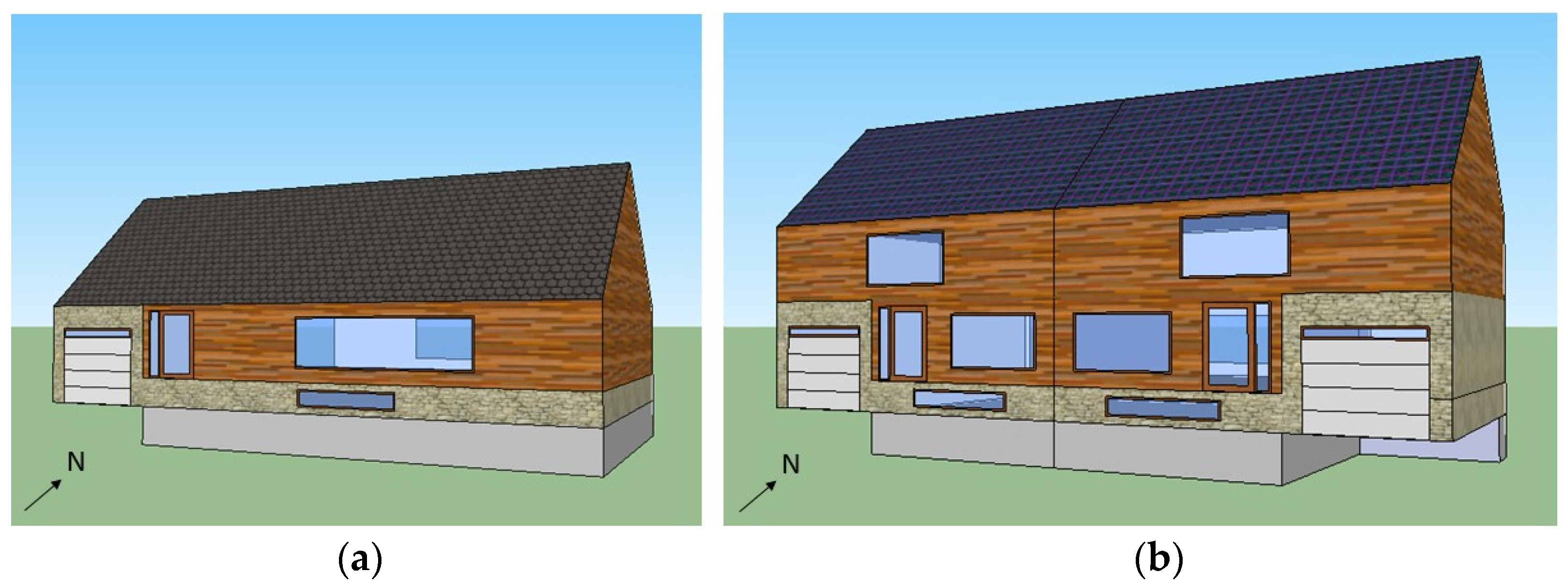
As a first step, the energy that is made available (or upgrade energy) by retrofitting and rebuilding an existing single-detached house to a low-energy solar house is quantified through annual energy simulations. Once the annual profile of upgrade energy is known, the maximum amount of electricity that can serve to decarbonize mobility is determined and the remainder is used for heating electrification.

Figure 3 illustrates the two main scenarios considered in this study. The first scenario uses the results for a single-detached house to estimate how many houses would need to be upgraded in Québec to provide all the energy required to electrify greenhouse operations. This includes the energy needed to convert all of the existing greenhouses from natural gas to electric heating and the electricity required to operate all of the planned new greenhouses (to achieve fresh vegetable production autonomy in Québec). The second scenario expands upon the findings of scenario 1 by considering the impact of upgrading all of the single-detached houses in Québec that employ electric resistance heating (42% of single-detached houses). Since all of the greenhouse operations have already been decarbonized in scenario 1, the additional upgrade energy would serve to electrify the heating in buildings that use natural gas for heating (e.g., commercial and institutional buildings). In all cases, the use of upgrade energy is first prioritized for decarbonizing mobility because it carries the highest GHG emissions and contributes to urban pollution the most.

Although the present analysis considers that all of the upgrade energy is saved by the utility, some the solar power generated on-site would likely be self-consumed by the building itself, used for the occupants’ EV, or to operate a greenhouse located the land lot (Figure 1). Increasing self-consumption may even be incentivized in certain low voltage grids to avoid power grid congestion. For the case where the house is fully operated using electricity (current situation), shifting energy use from the utility to consumption on-site would not change the net amount of upgrade energy and associated decarbonization potential presented in this investigation.

To quantify the decarbonization potential for the two main scenarios, the energy analysis is separated into different sections and the key assumptions for each can be found below. A house upgrade implies either a retrofit (efficiency measures applied while keeping the main structure) or a rebuild and the results for both are presented and compared. In addition, mobility decarbonization is achieved by switching to battery or fuel cell EVs and the results for both are provided.

• The first part covers the energy analysis of a single-detached house to answer the following questions:

  1.1.

  How much energy can be made available by upgrading an existing house to a low-energy solar house?

  1.2.

  What is the maximum amount of mobility electrification that is achieved using upgrade energy?

  1.3.

  How much energy is available for heating decarbonization and what is the maximum amount of greenhouse area that can be decarbonized/operated by using it?

• The second part consists of evaluating the impact of upgrading many houses to answer the following questions:

  2.1.

  Scenario 1: How many houses should be upgraded to provide enough energy for decarbonizing/operating all of the greenhouses needed to achieve fresh vegetable production autonomy in Québec?

  2.2.

  Scenario 1: How many houses should be upgraded to provide enough energy for decarbonizing/operating all of the greenhouses needed to achieve fresh vegetable production autonomy in Québec?

The details, parameter values, and key assumptions for the energy modeling are presented below and given in Table 3. The values for the modeled house are given in [7,24] for the greenhouse.

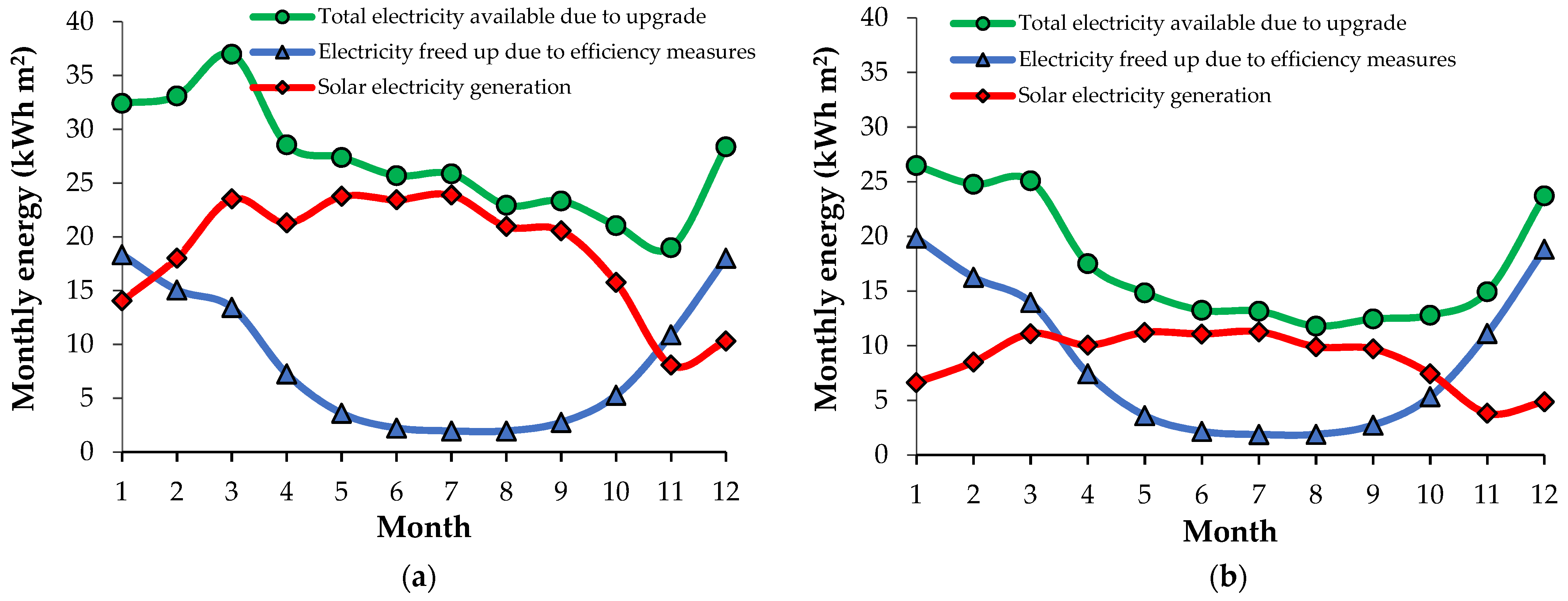
Section 1.1: For each hour of the year, the quantity of electricity that is freed up by implementing energy efficiency measures is calculated by subtracting the electricity consumed by the upgraded house from that of the existing house. The electricity that is made available for decarbonization (E_decarb in kWh year⁻¹) is found by summing the electricity that is freed up by implementing energy efficiency measures (E_eff in kWh year⁻¹) and the solar electricity generation (E_PV in kWh year⁻¹). The sum of these hourly values over one year provides the annual quantity of energy for the case where the house is retrofitted or rebuilt. Monthly totals are used to visualize and calculate some of the results.

Section 1.2: This study considers using a portion of the electricity that is made available from the house upgrade (or upgrade energy) to power battery or fuel cell electric vehicles (BEVs and FCEVs). Personal vehicles are assumed to be used for traveling approximately the same distance each day and modeled as a constant load throughout the year. The maximum amount of energy that can serve to electrify personal vehicles is taken as the lowest value of the monthly electricity (E_EV in kWh month⁻¹) that is made available from the house energy upgrade. A value of one month was selected for convenience and because the hydropower grid with large reservoirs allows it to provide energy flexibly. Therefore, each month, an amount of energy equal to E_EV is reserved for EVs. When the monthly value of upgrade energy exceeds E_EV, the surplus serves to electrify heating. The annual quantity of electricity that is available for EVs is E_EV multiplied by twelve.

The distance a BEV or FCEV can travel (D_EV in km year⁻¹) using the electricity that is provided by upgrading a single-detached house is given by:

$$D_{EV}=12·E_{EV}/E{C}_{EV}$$

(1)

where

• E_EV is the monthly energy reserved for EVs (kWh month⁻¹)
• EC_EV is the BEV or FCEV energy consumption (kWh km⁻¹)
• the factor 12 is the number of months per year (month year⁻¹).

The energy consumption (grid-to-wheel) for BEV (EC_BEV) was taken as the weighted value between cars (0.19 kWh km⁻¹ for 63% of personal vehicles) and light trucks (0.25 kWh km⁻¹ for 37% of personal vehicles) [31]. The energy consumption of a FCEV is estimated by comparing the efficiencies of BEV and FCEV for converting grid electricity into power at the wheels. The grid-to-wheel efficiency of a BEV is estimated to be 83% by multiplying the following efficiencies: 97% for the AC/DC inverter, 95% for the batteries, 97% for the DC/AC inverter, and 93% for the electric motor [32]. The grid-to-wheel efficiency of an FCEV is taken as 35% by multiplying the following efficiencies and assuming hydrogen is produced directly at the refuel station: 97% for the AC/DC inverter, 73% for water electrolysis, 92% for hydrogen compression, 60% for the fuel cell, 97% for the DC/AC inverter, and 93% for the electric motor [32,33]. The ratio of these efficiencies (R_BEV:FCEV) equals 2.37 (83%/35%), meaning that a FCEV requires that many times more energy than the BEV for a similar range. The energy consumption (EC_FCEV) of a personal FCEV is found by multiplying the energy consumption of a BEV (EC_BEV) by this ratio of efficiencies (R_BEV:FCEV). If the energy that is made available by upgrading a given number of houses exceeds the need for electrifying all the personal vehicles, then the surplus energy can be used to decarbonize other vehicles such as fuel cell electric trucks (FCET) for regional or long-haul transport. The energy consumption of a FCET (EC_FCET) is estimated the same way as for the FCEV using the energy consumption for battery electric trucks (BET) provided by Ref. [34].

Then, the number of BEVs or FCEVs that can be powered using the energy from a single house upgrade (N_EV) is calculated by:

$$N_{EV}=D_{EV}/D_{EV\_yr}$$

(2)

where D_{EV_yr} is the personal EV annual travel distance (km year⁻¹).

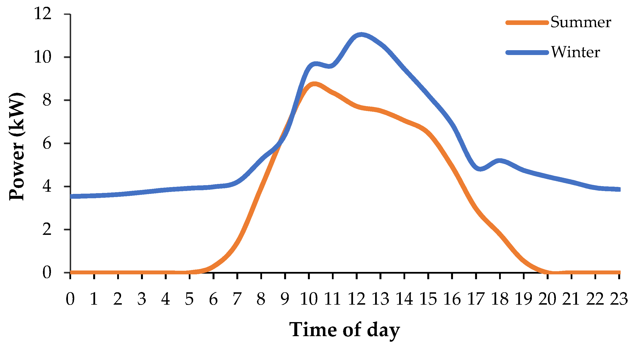
Section 1.3: The electricity that is made available by upgrading to a low energy solar house (or upgrade energy) is divided between mobility and heating decarbonization purposes. To satisfy the energy needs of the newly electrified heating loads, it is necessary to ensure that there is sufficient energy over the desired period and that enough power is available during peak demand. Therefore, the amount of heating decarbonization will be limited either by energy or power availability. The monthly amount of electricity that is available for heating decarbonization is found by subtracting the amount of electricity dedicated to EVs (E_EV in kWh month⁻¹) from the monthly amount of upgrade energy (E_{decarb_mo} in kWh month⁻¹). The amount of power available during periods of peak demand is found by subtracting the EV power demand from the maximum hourly value of power that is freed up by implementing energy efficiency measures. The contribution of solar energy is ignored as it is not guaranteed to be available during peak periods. The power demand from EV is assumed to be constant with time and calculated by dividing the monthly amount that is reserved for EV (E_EV in kWh month⁻¹) by the number of hours in one month.

The portion of the upgrade energy that is not used for EVs will be prioritized for use in greenhouses and any surpluses will then serve to electrify heating in other buildings. It is desired to determine the greenhouse area that can be decarbonized (for existing greenhouses) and operated (for new greenhouses) using the electricity that is made available by upgrading a single-detached house. Two cases are considered to address the different needs for decarbonizing the heating in existing greenhouses and providing low-emission power for the operation of new greenhouses (including heating, lighting, and other electricity needs).

The annual electricity that is available for greenhouses (E_GH in kWh year⁻¹) is given by:

$$E_{GH}=E_{decarb}-12·E_{EV}$$

(3)

where

• E_decarb is the electricity available from upgrading one house (kWh year⁻¹)
• the factor 12 is the number of months per year (month year⁻¹).

When the potential greenhouse area is designed based on energy availability, it is necessary to find the area (A_{GH_per_house} in m²) which minimizes the annual difference between the house upgrade energy and the actual energy consumed by a given greenhouse area. The greenhouse area based on power availability can be found by dividing the power that is dedicated to greenhouses (P_max in kW, obtained by subtracting the EV power demand (P_EV in kW) from the maximum power freed up by implementing efficiency measures (P_eff in kW)) by the greenhouse’s peak power demand per unit area (P_GH in kW m⁻²). The calculated greenhouse areas (A_{GH_per_house} calculated for existing and new greenhouse) based on energy and power are compared and the lowest value obtained is selected as the final design. The annual thermal energy consumed by the existing greenhouses (E_{GH_exist_per_house} in kWh year⁻¹) that are heated using the electricity that is made available from upgrading a house is determined from:

$$E_{GH\_exist\_per\_house}=A_{GH\_exist\_per\_house}·E_{GH\_heat}$$

(4)

where

• A_{GH_exist_per_house} is the greenhouse area that can be decarbonized from one house upgrade (m²)
• E_{GH_heat} is the electricity consumed for heating per unit area of a greenhouse (kWh m⁻² year⁻¹).

Similarly, the annual energy consumed by the new greenhouses (E_{GH_new_per_house} in kWh year⁻¹) that are operated using the upgrade energy may be written as:

$$E_{GH\_new\_per\_house}=A_{GH\_new\_per\_house}·E_{GH}$$

(5)

where

• A_{GH_new_per_house} is the greenhouse area that can be operated from one house upgrade (m²)
• E_GH is the electricity consumed per unit area of a greenhouse (kWh m⁻² year⁻¹).

Section 2.1: For scenario 1, it is desired to know how many houses would need to be upgraded to decarbonize/operate greenhouses in Québec. For the first case, it is desired to know how many houses would need to be upgraded to provide enough energy for electrifying the heating energy used in existing greenhouses, which are nearly all heated using natural gas today. For the second case, it is desired to know how many houses would need to be upgraded to provide enough energy to operate all of the new greenhouses (including heating, lighting, and other electricity needs) that will be built to achieve local fresh vegetable production autonomy.

Currently, a greenhouse area of approximately 1,280,000 m² is used to grow 41,000 t year⁻¹ of vegetables in Québec [29]. The government has plans and established financial incentives to achieve fresh vegetable production autonomy by doubling the greenhouse production area by 2025 [8,35]. Therefore, approximately 1,280,000 m² of additional greenhouse area would be needed to produce a total of 82,000 tonnes of vegetables per year.

The previous analysis determined the maximum greenhouse area that could be decarbonized/operated using the electricity that is made available by upgrading a house. The number of houses (N_{house_GH_exist}) needed to provide enough power for electrifying the heating in all existing greenhouses is estimated using:

$$N_{house\_GH\_exist}=A_{GH\_tot\_exist}/A_{GH\_exist\_per\_house}$$

(6)

where A_{GH_tot_exist} is the total existing greenhouse area (m²).

Similarly, the number of houses (N_{house_GH_new}) needed to provide enough electricity for operating all the new greenhouses is determined from:

$$N_{house\_GH\_new}=A_{GH\_tot\_new}/A_{GH\_new\_per\_house}$$

(7)

where A_{GH_tot_new} is the total new greenhouse area (m²).

The total number of houses that would need to be upgraded to provide enough electricity to decarbonize and operate all greenhouses in Québec (N_{house_GH_tot}) is defined as:

$$N_{house\_GH\_tot}=N_{house\_GH\_exist}+N_{house\_GH\_new}$$

(8)

The fraction of total single-detached houses that would need to be upgraded (F_{upgraded_GH} in %) is derived from:

$$F_{upgraded\_GH}=100·N_{house\_GH\_tot}/N_{house\_tot}$$

(9)

where

• N_{house_tot} is the total number of single-detached homes in Québec
• the factor 100 serves to express the result in percentage.

The total electricity that is available for decarbonization (E_{decarb_tot} in TWh year⁻¹) is calculated as:

$$E_{decarb\_tot}=E_{decarb}·N_{house\_GH\_tot}/{10}^9$$

(10)

where

• E_decarb is the electricity that is available for decarbonization (kWh year⁻¹)
• the factor 10⁹ serves to convert kWh to TWh (month year⁻¹).

The fraction of total electricity consumption (F_decarb in %) is determined by dividing total electricity that is available for decarbonization (E_{decarb_tot}) by the total electricity consumption in Québec (E_QC in TWh year⁻¹) and multiplying this by 100 to express the result in percentage.

The total electricity consumed for decarbonizing the existing greenhouses and operating the new greenhouses (E_{GH_tot} in TWh year⁻¹) is computed as:

$$E_{GH\_tot}=\left(E_{GH\_exist\_per\_house}·N_{house\_GH\_exist}+E_{GH\_new\_per\_house}·N_{house\_GH\_new}\right)/{10}^9$$

(11)

where the factor 10⁹ serves to convert kWh to TWh (month year⁻¹).

Later, the electricity (E_{GH_heat_tot} in TWh year⁻¹) that is used solely for heating the existing and new greenhouses will be needed to determine the avoided GHG emissions and is described by:

$$E_{GH\_heat\_ tot}=\left(E_{GH\_exist\_per\_house}·N_{house\_GH\_exist}+A_{GH\_new\_per\_house}·E_{GH\_heat}·N_{house\_GH\_new}\right)/{10}^9$$

(12)

where the factor 10⁹ serves to convert kWh to TWh (month year⁻¹).

The total electricity for EV (E_{EV_tot} in TWh year⁻¹) is calculated by:

$$E_{EV\_ tot}=12·E_{EV}·N_{house\_GH\_tot}/{10}^9$$

(13)

where the factors 12 is the number of months per year (month year⁻¹) and 10⁹ serves to convert kWh to TWh (month year⁻¹).

The leftover electricity (E_leftover in TWh year⁻¹) and available for other decarbonization purposes such as electrifying heating in buildings that employ natural gas is expressed as:

$$E_{leftover}=E_{decarb\_tot}-E_{GH\_tot}-E_{EV\_ tot}$$

(14)

The number of BEVs or FCEVs that can be powered using a portion of the electricity that is made available by upgrading these houses (N_{EV_tot}) is given by:

$$N_{EV\_tot}=N_{EV}·N_{house\_GH\_tot}$$

(15)

The fraction of total personal vehicles that could be converted to EVs (F_{EV_tot} in %) is estimated using:

$$F_{EV\_tot}=100·N_{EV\_tot}/N_{PV\_tot}$$

(16)

where

• N_{PV_tot} is the total number of personal vehicles
• the factor 100 serves to express the result in percentage.

Section 2.2: For scenario 2, it is desired to quantify the potential decarbonization that can be achieved by converting all of the single-detached houses that employ electric resistance heating to low energy solar houses. This scenario builds upon the results of scenario 1, where a certain number of houses are upgraded to provide energy for greenhouses. In addition to this, scenario 2 includes the decarbonization potential of an additional number of houses (N_{house_added}) equal to:

$$N_{house\_added}=N_{house\_EH\_tot}-N_{house\_GH\_tot}$$

(17)

where N_{house_EH_tot} is the number of houses that use electric resistance heating.

The analysis for these additional houses follows a similar procedure as for scenario 1 and uses the same equations, Equations (10), (13) and (14) (where E_{GH_tot} is ignored), (15), and (16), but using N_{house_added} instead of N_{house_GH_tot}. The total values for scenario 2 are the sum of the contributions from N_{house_GH_tot} and N_{house_added}.

2.5. GHG Emissions Analysis

This section aims to quantify the reduction in GHG emissions that is achieved by decarbonizing mobility and heating using the energy that is made available by upgrading the number of houses that were determined in scenarios 1 and 2. The analysis also includes estimating the embodied emissions associated with the house upgrades and electrified loads and determining the emissions payback time.

GHG emissions avoided by decarbonization

The reduction in emissions from mobility electrification (GHG_{EV_per_house} in tCO_2eq) that can be achieved using a portion of the upgrade energy is determined from:

$$GH{G}_{EV\_per\_house}=D_{EV}·F{E}_{PV}·E{F}_{PV}/1000$$

(18)

where

• FE_PV is the average fuel efficiency of personal vehicles (L km⁻¹)
• EF_PV is the emissions factor of gasoline-powered personal vehicles (kgCO_2eq L⁻¹)
• the factor 1000 serves to convert kg to tonne (t).

If the portion of upgrade energy that can be dedicated to EVs exceeds the energy needs of all of the personal vehicles in Québec, the surplus is assumed to be used for decarbonizing long-haul trucks by switching them to fuel cell electric trucks (FCETs). The associated reduction in emissions (GHG_FCET in MtCO_2eq year⁻¹) is estimated using:

$$GH{G}_{FCET}=E_{FCET}/E{C}_{FCET}·F{E}_T·E{F}_T/1000/{10}^6$$

(19)

where

• E_FCET is the surplus electricity available for FCETs (kWh year⁻¹)
• EC_FCET is the FCET energy consumption (kWh km⁻¹)
• FE_T is the average fuel efficiency of a diesel-powered truck (L km⁻¹)
• EF_T is the emissions factor of diesel-powered truck (kgCO_2eq L⁻¹)
• the factor 1000 serves to convert kg to tonne (t)
• the factor 10⁶ serves to convert tonnes (t) to megatonnes (Mt).

The reduction in emissions that can be achieved by electrifying mobility (GHG_EV in MtCO_2eq year⁻¹) in scenario 1 (N_{house_GH_tot}) or scenario 2 (N_{house_EH_tot}) is given by:

$$GH{G}_{EV}=GH{G}_{EV\_per\_house}·N_{house}/{10}^6+GH{G}_{FCET}$$

(20)

where the factor 10⁶ serves to convert tonnes (t) to megatonnes (Mt).

The reduction in emissions (GHG_GH in MtCO_2eq year⁻¹) from electrifying the heating in existing greenhouses and from the emissions that are avoided by employing electric heating in the new greenhouses (assuming they would otherwise be heated using natural gas burned inside the greenhouse) is calculated by:

$$GH{G}_{GH}=E_{GH\_heat\_ tot}·{10}^9·E{F}_{NG}/\left(EV/3.6\right)/1000/{10}^6$$

(21)

where

• EF_NG is the emissions factor of natural gas (kgCO_2eq m⁻³)
• EV is the energy value of natural gas (MJ m⁻³)
• the factor 10⁹ serves to convert TWh to kWh
• the factor 3.6 serves to convert MJ to kWh
• the factor 1000 serves to convert kg to tonne (t)
• the factor 10⁶ serves to convert tonnes (t) to megatonnes (Mt).

The analysis considers that existing heating systems that burn natural gas directly inside the greenhouse are replaced with electric resistance heating. The use of heat pumps (e.g., geothermal or thermal storage using surplus air thermal energy) and dual fuel systems could be considered in future studies.

The reduction in emissions that is achieved using the leftover electricity (GHG_leftover in MtCO_2eq year⁻¹) to convert building heating from natural gas boilers to electric heat pumps is approximated by:

$$GH{G}_{leftover}=E_{leftover}·{10}^9/\eta ·COP·E{F}_{NG}/\left(EV/3.6\right)/1000/{10}^6$$

(22)

where

• η is the natural gas boiler efficiency (dimensionless)
• COP is the average coefficient of performance of an electric heat pump (MJ m⁻³)
• the factor 10⁹ serves to convert TWh to kWh
• the factor 3.6 serves to convert MJ to kWh
• the factor 1000 serves to convert kg to tonne (t)
• the factor 10⁶ serves to convert tonnes (t) to megatonnes (Mt).

The total reduction in emissions (GHG_tot in MtCO_2eq year⁻¹) is equal to:

$$GH{G}_{tot}=GH{G}_{EV}+GH{G}_{GH}+GH{G}_{leftover}$$

(23)

The reduction in Québec’s emissions (R_GHG in %) is expressed as:

$$R_{GHG}=100·GH{G}_{tot}/GH{G}_{QC}$$

(24)

where

• GHG_QC is Québec’s total annual GHG emissions (MtCO_2eq year⁻¹)
• the factor 100 serves to express the result in percentage.

Embodied GHG emissions

This study considers the emissions that are required for the house upgrade and the production of EVs. The embodied energy of the new greenhouses will not be considered because they will be built regardless of the decarbonization scenario. They will be treated like the existing greenhouses, whereby the embodied emissions produced by converting the heating system from natural gas to electric resistance are relatively small and can be neglected.

The embodied emissions produced by retrofitting or rebuilding the houses (EE_houses in MtCO_2eq) in scenario 1 (N_{house_GH_tot}) or scenario 2 (N_{house_EH_tot}) is calculated by:

$$E{E}_{houses}=N_{house}·E{E}_{house\_m2}·A/1000/{10}^6$$

(25)

where

• EE_house is the embodied emissions per unit area for a retrofitted or rebuilt house (kgCO_2eq m⁻²)
• A is the living area of the house (m²)
• the factor 1000 serves to convert kg to tonne (t)
• the factor 10⁶ serves to convert tonnes (t) to megatonnes (Mt).

The operational (e.g., O&M) and downstream processes (e.g., removal/recycling) for roof-mounted PV systems are small compared to the upstream emissions (e.g., production-related) and ignored in this study [36]. The embodied emissions produced by the PV system (EE_PV in MtCO_2eq) in scenario 1 (N_{house_GH_tot}) or scenario 2 (N_{house_EH_tot}) is estimated using:

$$E{E}_{PV}=N_{house}·E{E}_{PV\_m2}·A_{PV}/1000/{10}^6$$

(26)

where

• EE_{PV_m2} is the embodied emissions per unit area of the PV system (kgCO_2eq m⁻²)
• A_PV is PV area (m²)
• the factor 1000 serves to convert kg to tonne (t)
• the factor 10⁶ serves to convert tonnes (t) to megatonnes (Mt).

The embodied emissions related to the production of FCETs (EE_FCETs in MtCO_2eq) is determined from:

$$E{E}_{FCETs}=E_{FCET}/E{C}_{FCET}/D_{ET\_yr}·E{E}_{FCET}/1000/{10}^6$$

(27)

where

• D_{ET_yr} is the FCET annual travel distance (km year⁻¹)
• EE_FCET is the embodied emissions per truck (kgCO_2eq)
• the factor 1000 serves to convert kg to tonne (t)
• the factor 10⁶ serves to convert tonnes (t) to megatonnes (Mt).

The embodied emissions related to the production of EVs (EE_EVs in MtCO_2eq) in scenario 1 (N_{house_GH_tot}) or scenario 2 (N_{house_EH_tot}) is computed as:

$$E{E}_{EVs}=N_{EV}·N_{house}·E{E}_{EV}/1000/{10}^6+E{E}_{FCETs}$$

(28)

where

• the factor 1000 serves to convert kg to tonne (t)
• the factor 10⁶ serves to convert tonnes (t) to megatonnes (Mt).

The total embodied emissions (EE_tot in MtCO_2eq) are approximated by:

$$E{E}_{tot}=E{E}_{houses}+E{E}_{PV}+E{E}_{EVs}$$

(29)

Emissions payback time

The emissions payback time (PT_GHG in yr) is equal to:

$$P{T}_{GHG}=E{E}_{tot}/GH{G}_{tot}$$

(30)

Table 3. Parameter values used in the model.

Parameter	Value	Reference
Living area of existing, retrofitted and rebuilt houses (A)	140 m2	[7]
PV area (APV) (value for rebuilt house in parenthesis)	97.7 (46.1) m2	[7]
BEV energy consumption for (ECBEV)	0.22 kWh km−1	[31]
FCEV energy consumption for (ECFCEV)	0.52 kWh km−1	Calculated
BET energy consumption for (ECBET)	1.15 kWh km−1	[34]
FCET energy consumption for (ECFCET)	2.73 kWh km−1	Calculated
Electric vehicle annual travel distance (DEV_yr)	14,800 km year−1	[37]
Electric truck annual travel distance (DET_yr)	120,000 km year−1	[34]
Total number of personal vehicles (NPV_tot)	5,400,000	[38]
Total number of single-detached houses (Nhouse_tot)	1,735,000	[39]
Single-detached houses with electric resistance heating (Nhouse_EH_tot)	734,000	[39]
Emissions factor for gasoline-powered personal vehicles (EFPV)	2.3 kgCO2eq L−1	[31]
Average fuel efficiency for personal vehicles (FEPV)	0.1 L km−1	[37]
Emissions factor for diesel-powered trucks (EFT)	2.7 kgCO2eq L−1	[40]
Average fuel efficiency for trucks (FEPV)	0.4 L km−1	[41]
Emissions factor for natural gas (EFNG)	1.9 kgCO2eq m−3	[42]
Energy value of natural gas (EV)	37 MJ m−3	[43]
Boiler efficiency (η)	0.8	[44]
Average COP of electric heat pump (COP)	3	[3]
Total electricity consumption in Québec (EQC)	174.6 TWh year−1	[1]
Total annual GHG emissions in Québec (GHGQC)	82 MtCO2eq	[1]
Embodied emissions for house rebuilds (EEhouse_rebuild_m2)	600 kgCO2eq m−2	[45]
Embodied emissions for house retrofits (EEhouse_retrofit_m2)	120 kgCO2eq m−2	[21]
PV system embodied emissions (EEPV_m2)	300 kgCO2eq m−2	[46]
Embodied emissions per BEV (EEBEV)	9900 kgCO2eq	[47]
Embodied emissions per FCEV (EEFCEV)	7400 kgCO2eq	[47]
Embodied emissions per FCET (EEFCET)	148,000 kgCO2eq	Estimated based on weight

Table 3. Parameter values used in the model.

Parameter	Value	Reference
Living area of existing, retrofitted and rebuilt houses (A)	140 m2	[7]
PV area (APV) (value for rebuilt house in parenthesis)	97.7 (46.1) m2	[7]
BEV energy consumption for (ECBEV)	0.22 kWh km−1	[31]
FCEV energy consumption for (ECFCEV)	0.52 kWh km−1	Calculated
BET energy consumption for (ECBET)	1.15 kWh km−1	[34]
FCET energy consumption for (ECFCET)	2.73 kWh km−1	Calculated
Electric vehicle annual travel distance (DEV_yr)	14,800 km year−1	[37]
Electric truck annual travel distance (DET_yr)	120,000 km year−1	[34]
Total number of personal vehicles (NPV_tot)	5,400,000	[38]
Total number of single-detached houses (Nhouse_tot)	1,735,000	[39]
Single-detached houses with electric resistance heating (Nhouse_EH_tot)	734,000	[39]
Emissions factor for gasoline-powered personal vehicles (EFPV)	2.3 kgCO2eq L−1	[31]
Average fuel efficiency for personal vehicles (FEPV)	0.1 L km−1	[37]
Emissions factor for diesel-powered trucks (EFT)	2.7 kgCO2eq L−1	[40]
Average fuel efficiency for trucks (FEPV)	0.4 L km−1	[41]
Emissions factor for natural gas (EFNG)	1.9 kgCO2eq m−3	[42]
Energy value of natural gas (EV)	37 MJ m−3	[43]
Boiler efficiency (η)	0.8	[44]
Average COP of electric heat pump (COP)	3	[3]
Total electricity consumption in Québec (EQC)	174.6 TWh year−1	[1]
Total annual GHG emissions in Québec (GHGQC)	82 MtCO2eq	[1]
Embodied emissions for house rebuilds (EEhouse_rebuild_m2)	600 kgCO2eq m−2	[45]
Embodied emissions for house retrofits (EEhouse_retrofit_m2)	120 kgCO2eq m−2	[21]
PV system embodied emissions (EEPV_m2)	300 kgCO2eq m−2	[46]
Embodied emissions per BEV (EEBEV)	9900 kgCO2eq	[47]
Embodied emissions per FCEV (EEFCEV)	7400 kgCO2eq	[47]
Embodied emissions per FCET (EEFCET)	148,000 kgCO2eq	Estimated based on weight

3. Results and Discussion

3.1. Energy Available by Upgrading a House

As expected, energy efficiency upgrades significantly reduce a house’s energy consumption. The retrofitted and rebuilt houses consume similar amounts of energy, equal to about 65% less than an existing house. As shown in

Table 4. Energy and peak power that is made available from retrofitting/rebuilding a single-detached house.

Item	Existing	Retrofit	Rebuild
House energy use (kWh year−1)	22,557	8435	7846
Energy freed up due to efficiency (kWh year−1)	-	14,122	14,711
Solar energy generation (kWh year−1)	-	31,323	14,793
Total energy made available due to upgrade (kWh year−1)	-	45,445	29,504
Fraction of energy provided by efficiency measures	-	31%	50%
Fraction of energy made available that is from PV	-	69%	50%
Power made available due to efficiency measures (kW)	-	7.1	7.3

, implementing efficiency measures in single-detached houses results in around 14,000 kWh year⁻¹ of electricity being freed up and available for decarbonization elsewhere. In addition, the retrofitted and rebuilt houses generate approximately 14,800 kWh year⁻¹ and 31,300 kWh year⁻¹ of solar electricity on-site, respectively. This large difference is caused by the retrofitted house having a PV area more than double the size of the rebuilt house. The simulated solar energy production for the rebuilt house (14,800 kWh year⁻¹) is in good agreement with a simple calculation that yields 15,500 kWh year⁻¹ based on the annual global radiation on a south-facing surface at a tilt angle equal to the latitude for Montreal (4.35 kWh m⁻² year⁻¹) provided by Ref. [48], a PV module efficiency of 21.16%, and a PV area of 46.1 m².

The total electricity that is made available by upgrading one house (or upgrade energy) equals the sum of the energy freed up by implementing energy efficiency measures and the solar energy generation. This amounts to approximately 45,500 kWh year⁻¹ per retrofitted house and 29,500 kWh year⁻¹ per rebuilt house. In other words, the retrofitted house could provide energy for decarbonization that is equal to twice the electricity consumption of the existing house and 1.3 times more for the rebuilt house. Solar energy provides 50% and nearly 70% of the total upgrade energy for the retrofitted and rebuilt houses, respectively, with the remainder provided by the efficiency measures. Meanwhile, the amount of energy that is freed up due to efficiency is highest during periods of peak demand in winter and is found to be 7.1 and 7.3 kW per retrofitted and rebuilt house, respectively. When the electricity that is made available by upgrading to a low-energy solar house is used to decarbonize elsewhere, the amount of energy and peak power that is required for the electrified load must not exceed these values.

Figure 4 provides the monthly quantity of electricity that is freed up by implementing energy efficiency measures, from solar electricity generation, and the total electricity that is made available by retrofitting (Figure 4a) and rebuilding (Figure 4b) a house. As expected, the energy that is freed up by implementing efficiency measures is greatest in the winter months because heating is the largest contributor to total energy use and is therefore reduced most. The opposite trend occurs with solar energy, whereby energy production in summer is about 2–3 times more than in winter for sloped south-facing roofs. The annual profile of the total upgrade energy is highest in winter due to the relatively large contribution from the energy efficiency measures during that period. The impact of a larger PV system can be observed by comparing the total electricity profile (green line) for the retrofitted house (Figure 4a) and the rebuilt house (Figure 4b). The profile’s U-shape is better defined for the rebuilt house because of a lower amount of solar electricity is generated compared to the electricity that is freed up from efficiency measures.

The use of upgrade energy is prioritized for electrifying mobility because transportation is the largest single contributor to health-damaging air pollution in cities. Since EVs typically require a near-constant supply of energy year-round, the minimum annual value of the monthly upgrade energy is what dictates the amount that can be dedicated to EVs. Energy efficiency measures alone provide little energy for EV mobility due to the low availability in summer. For solar energy, the opposite effect occurs, where minimum energy availability occurs in winter, and this would dictate the portion that can be available for EVs. The combination of the electricity that is freed up by implementing energy efficiency measures and the solar electricity generation is a promising way to obtain a larger amount of energy for EVs than would be provided by each of the energy supply streams separately. This symbiosis occurs because the minimum value of monthly energy for one is close to the maximum of the other. For example, for the retrofitted house, energy efficiency (blue line in Figure 4a) provides a minimum value of 2 kWh m⁻² month⁻¹ (in summer) and this is what limits the electricity that can be reserved year-round for EVs. For solar electricity generation (red line in Figure 4a), the minimum value is 8 kWh m⁻² month⁻¹ in November. However once combined (green line in Figure 4a), the minimum value becomes 19 kWh m⁻² month⁻¹ (in November), which is 90% more than the sum of the minimum values for efficiency and solar individually (total of 10 kWh m⁻² month⁻¹). Therefore, the efficiency and solar combo can achieve the desired goal of attributing a greater share of the total upgrade energy for EV, and the remainder is concentrated in winter and is ideal for heating decarbonization (Figure 5). It would be possible to use an alternative source of energy such as biomass to assist solar electricity production in winter (neglects efficiency) or to complement efficiency in summer (neglects solar) to achieve a constant annual energy profile. However, this study focuses on how to employ energy from building upgrades as the sole means for providing energy needed for decarbonization.

As illustrated in Figure 5, the process of upgrading residential buildings to low-energy solar buildings provides an energy profile that is suitable for both mobility and heating decarbonization. The relative proportion of energy that is freed up by implementing various efficiency measures and solar energy generation is what determines how much energy is available for the desired decarbonization application(s).

It should be noted that the energy consumption of an existing house is representative of a recently built house. More energy would be freed up by implementing energy efficiency measures if older, less efficient houses are selected for the analysis. Therefore, this paper provides conservative estimates that are more representative of what could be expected in the future, when recently built houses will be renovated or rebuilt. Additionally, a portion of solar energy generation would usually be consumed on-site (self-consumption) to minimize energy transactions with the grid and peak demand. Although it is assumed they would be implemented, these grid-interactive flexibility and self-consumption strategies were not considered in the analysis as they would not significantly impact the quantity of house upgrade energy. In addition, separating them enables a better understanding of how each energy supply stream contributes to the profile of the house upgrade energy.

3.2. Heating Decarbonization

The electricity that is made available by upgrading to a low-energy solar building will be used to electrify mobility and heating. Figure 6 illustrates the energy profiles that are made available for mobility and heating decarbonization by retrofitting (Figure 6a) and rebuilding (Figure 6b) an existing single-detached house. A greater amount of electricity is provided by the retrofitted house because it has a larger PV system that generates over two times more solar electricity than the rebuilt house.

As a first step (scenario 1), this study investigates the case where the electricity would be used to decarbonize the heating energy used in existing greenhouses and provide the electricity required to operate the new greenhouses needed to grow all fresh vegetables locally.

Table 5. Greenhouse (GH) area that can be decarbonized/operated using the energy that is made available from retrofitting/rebuilding a single-detached house.

Item	Retrofit		Rebuild
	Analysis for Electrifying Heating in Existing Greenhouses	Analysis for the Energy Needs of New Greenhouses	Analysis for Electrifying Heating in Existing Greenhouses	Analysis for the Energy Needs of New Greenhouses
Energy made available by upgrading a house (Edecarb kWh year−1)	45,445	45,445	29,505	29,505
Freed up power due to efficiency measures (Peff kW)	7.1	7.1	7.3	7.3
Average power reserved for EV (PEV kW)	3.6	3.6	2.3	2.3
Peak power available for GH (Pmax kW)	3.5	3.5	5	5
GH peak load (PGH kW m−2)	0.28	0.5	0.28	0.5
GH area possible based on peak demand (AGH_per_house m2)	12.5	7	18	10.1
GH area possible based on energy availability (AGH_per_house m2)	19.8	14.6	14.1	10.4
GH design based on: energy or peak?	peak	peak	energy	peak
Electricity use for GH heating (kWh year−1)	8555	4791	9650	6912
Other electricity used for GH (kWh year−1)	N/A	1681	N/A	2426
Fraction of total energy available consumed for GH	19%	14%	33%	32%
Electricity leftover for other decarbonization (kWh year−1)	4973	7056	31	343
Fraction of total energy available for other	11%	16%	0.1%	1.2%

provides the greenhouse area that can be decarbonized/operated using the electricity that is made available by upgrading a single-detached house. The greenhouse area is selected as the minimum value that is calculated based on available energy and peak power demand. It was found that the energy provided by a house retrofit could provide enough electricity to heat 12.5 m² of the existing greenhouse and operate 7 m² of the new greenhouse. Both of these areas were selected based on the availability of peak power. Rebuilding a house can provide enough electricity to heat 14.1 m² of existing greenhouse (selected based on energy availability) and to operate 10.1 m² of new greenhouse (selected based on peak power availability).

The upgrade energy that is not used for decarbonizing mobility and greenhouses would be available for other decarbonization purposes. Since this surplus is predominantly available during the heating months, it can serve to electrify heating in other buildings, for instance converting a natural gas boiler to an electric heat pump. Figure 7 illustrates the differences that occur between the energy that is available for heating decarbonization and the energy consumed for the greenhouse when it is designed based on peak power (Figure 7a) and based on energy availability (Figure 7b). The two lines show how a better overlapping of energy supply and demand results in more energy being used for the greenhouses (i.e., less surplus available for electrifying heating elsewhere). When the greenhouse design is based on energy availability, there is very little surplus energy for decarbonization elsewhere. The opposite typically occurs for greenhouse areas designed based on peak power, where up to 16% of the upgrade energy is available for other decarbonization purposes (Table 5 and Figure 7a). A possible solution for using more of the upgrade energy for greenhouse purposes (i.e., in the case where the design is based on peak availability) is to employ a dual heating system, which would switch to an alternative fuel such as biomass to provide heat below a predetermined exterior air temperature. As shown in Figure 7b, there will be some months where the greenhouse energy consumption is greater than the energy that is available from the house upgrade. These periods would be supplied from the surplus that is available during the other parts of the year (e.g., surplus energy in winter covers the deficit in fall).

It should be noted that this is possible owing to the flexible nature of Québec’s hydropower system, which has large reservoirs that provide significant energy storage capacity. Hydroelectricity production can be reduced to accommodate distributed energy generation (e.g., from PV) and this saved energy (in the form of water stored in a reservoir) can be used at a later time (e.g., when the greenhouse energy consumption exceeds the amount that is available from building energy upgrades). The exceptionally large water reservoirs in Québec could enable seasonal grid energy balancing without the need for other forms of energy storage. Nuclear power plants would operate in a similar manner, where unused uranium can be stored for later use.

The electricity needed to electrify heating in existing greenhouses and to operate the new greenhouses would require 2.1 TWh year⁻¹ of electricity and would add nearly 1000 MW of peak demand to the existing grid. This represents a 2.6% increase compared to today’s peak demand of approximately 39,000 MW [5], or half of the new peak demand that is predicted to be required in the province by 2029 [15]. As shown in

Table 6. Energy that is provided by upgrading enough houses to achieve greenhouse (GH) crop production autonomy (scenario 1) and all houses heated by electric resistance (scenario 2).

Item	Scenario 1		Scenario 2
	Retrofit	Rebuild	Retrofit	Rebuild
House upgrades needed to electrify heating in existing GH (Nhouses_GH_exist)	102,000	90,000	102,000	90,000
Houses upgrades needed to operate new GH (Nhouses_GH_new)	183,000	126,000	183,000	126,000
Other houses to be upgraded in scenario 2 (Nhouses_added)	N/A	N/A	449,000	518,000
Total houses to be upgraded (Nhouses_GH_tot or Nhouses_tot2)	285,000	216,000	734,000	734,000
Fraction of total single-detached homes upgraded (Fupgraded)	16%	12%	42%	42%
Energy that is made available for GH (EGH_tot TWh year−1)	2.1	2.1	2.1	2.1
Energy that is made available for EV (EEV_tot TWh year−1)	9.1	4.3	23.4	14.6
Energy leftover for other decarbonization (Eleftover TWh year−1)	1.8	0	7.9	5.1
Total energy available from upgraded homes (Edecarb_tot TWh year−1)	13	6.4	33.4	21.8
Fraction of Quebec total electricity use made available (Fdecarb)	7%	4%	19%	12%

, all the energy needed to have an entirely local and decarbonized supply of fresh vegetables can be achieved by retrofitting 16% or rebuilding 12% of single-detached homes in Québec, respectively.

The second scenario considers the impact of upgrading all of the single-detached houses that currently use electric resistance heating in Québec (42% of the total or 734,000 houses). This would provide 7.9 and 5.1 TWh year⁻¹ of surplus electricity for decarbonizing heating in other buildings for the retrofitted and rebuilt houses, respectively. The total energy that is made available by retrofitting and rebuilding these houses equals 33.4 and 21.8 TWh year⁻¹ or 19% and 12% of the total electricity consumption of the province, respectively.

The analysis considers the case where PV is only applied to house roof surfaces. For multi-story residential buildings such as apartments, the available solar energy collection area may not be enough for providing the desired energy profile of the electrified load. In such cases, solar energy can be generated from other surfaces within a district, for instance solar carports or semi-transparent PV cladding for greenhouses. Using this cladding causes the greenhouse lighting energy to increase in winter. However, on an annual basis, it reduces the overall demand for electricity by potentially covering all lighting electricity needs [11].

3.3. Mobility Decarbonization

The energy that is reserved for electrifying mobility (which requires a constant supply of energy year-round) is taken as the minimum monthly value of the house upgrade energy (see Section 3.1 for additional details).

Table 7. Number of personal EVs that can be operated using the energy that is made available from retrofitting/rebuilding a single-detached house.

Item	Retrofit	Rebuild
Monthly energy reserved for EVs (EEV kWh month−1)	2660	1652
Annual energy for EVs (12 EEV kWh year−1)	31,917	19,824
Fraction of house upgrade energy that is consumed for EVs	70%	67%
Travel distance for BEV (DBEV km year−1)	145,078	90,107
Travel distance for FCEV (DFCEV km year−1)	61,379	38,122
Number of BEVs powered by one house upgrade (NBEV)	9.8	6.1
Number of FCEVs powered by one house upgrade (NFCEV)	4.1	2.6

provides the quantity of energy that can be dedicated to electrifying mobility and the number of EVs that can be operated using the energy that is made available from retrofitting/rebuilding a single-detached house. The maximum amount of energy that can be dedicated to EVs is found to be 2660 kWh month⁻¹ for the retrofitted house and 1652 kWh month⁻¹ for the rebuilt house. The rebuilt house provides 38% less energy for EVs than the retrofit house because less solar electricity is generated by its smaller roof area. Approximately 70% of the house upgrade energy can serve to electrify mobility. This energy is sufficient to power 9.8 and 6.1 personal BEVs for the retrofitted and rebuilt houses, respectively. For FCEVs, this energy is sufficient to power 4.1 and 2.6 personal vehicles for the retrofitted and rebuilt houses, respectively. The lower values for FCEVs are due to their lower well-to-wheel efficiency compared to BEV (35% versus 82%).

Table 8. Mobility electrification that can be achieved by upgrading enough houses for greenhouse crop production autonomy (scenario 1) and by upgrading all houses that employ electric resistance heating (scenario 2).

	Scenario 1		Scenario 2
	Retrofit	Rebuild	Retrofit	Rebuild
Fraction of total single detached homes upgraded (Fupgraded)	16%	12%	42%	42%
Energy available for EV (EEV_tot TWh year−1)	9.1	4.3	23.4	14.6
Number of BEVs (NEV_tot)	2,793,735	1,315,082	7,195,092	4,468,843
Number of FCEVs (NFCEV_tot)	1,181,965	556,381	3,044,077	1,890,664
Fraction of total personal vehicles replaced with BEV (FEV_tot)	52%	24%	133%	83%
Fraction of total personal vehicles replaced with FCEV (NFCEV_tot)	22%	10%	56%	35%

provides the amount of energy that can be used to power EVs for scenarios 1 and 2. If enough houses would be upgraded to provide greenhouse fresh vegetable production autonomy (scenario 1), then 9.1 and 4.3 TWh year⁻¹ of electricity would be available to decarbonize mobility for the retrofitted and rebuilt house, respectively. This would provide enough energy to convert 52% and 24% of personal vehicles to BEVs and 22% and 10% to FCEVs for the retrofitted and rebuilt house, respectively.

If all houses that employ electric resistance heating would be upgraded (scenario 2), then 23.4 and 14.6 TWh year⁻¹ of electricity would be available to decarbonize mobility for the retrofitted and rebuilt house, respectively. This would provide enough energy to convert 133% and 83% of personal vehicles to BEVs and 56% and 35% to FCEVs for the retrofitted and rebuilt house, respectively. For the case where BEVs are powered using energy that is made available by retrofitting houses, there is more than enough energy to cover all the energy required for personal vehicles. This surplus energy can be used for other mobility electrification purposes such as producing hydrogen for long-haul fuel cell electric trucks.

Figure 8 shows the profile of power that is made available by rebuilding a house, on a sunny summer and winter day. In winter (blue line), the energy efficiency measures free up electricity all day plus there is a contribution from solar electricity generation. In summer (orange line), upgrade energy is provided almost entirely by solar electricity generation (energy efficiency lowers electricity use mainly by employing a heat pump for DHW heating but this is often outweighed by the higher cooling energy requirements of the upgraded houses when there is no sun).

EV power demand is more or less constant throughout the year but may vary significantly throughout the day depending on the BEV’s charging schedule and hydrogen production times. Typically, BEVs would be charged during the day when people arrive at work or when they are at home. The power demand due to charging can increase quickly depending on the charging speed and the number of vehicles charging simultaneously. For instance, for the retrofitted house in scenario 2, if BEVs charge over one day (slow charge), over 6 h (typical charging time), and 2 h (fast charge), the power demand of Québec’s grid increases by 7%, 27%, and 82%, respectively. Therefore, the daily energy consumption profile for EVs would not necessarily match what is made available from the building upgrades. Most of the time, these short-term differences between energy supplied by low-energy solar houses and energy demand for EV could be accommodated by the grid owing to the flexible nature of hydropower with large reservoirs.

However, depending on the EV market penetration and the charging/refuelling times, the additional power demand for EVs can exceed grid power supply capabilities, particularly during periods of peak demand when the grid is already under pressure. Therefore, precautionary measures would be needed to ensure that EV charging/refuelling does not cause issues as the demand for power approaches the grid’s peak supply capabilities (e.g., during cold winter days). This can be achieved possibly by providing incentives to vehicle owners to slow charge over a longer period and/or charge during off-peak periods (e.g., avoid charging during the winter’s morning peak of 6–9 a.m. and evening peak of 4–8 p.m.). Other methods such as Hydro-Québec’s dynamic pricing incentivize consumers to reduce demand during peak periods upon receiving a signal from the utility [16]. These incentives could help to increase the economic appeal and adoption of dual heating systems, such as switching to biomass for heating buildings and greenhouses during the coldest periods of the year. Otherwise, additional grid power can be provided by building more peaking power plants but they are often costly to operate due to their low utilization factor.

The issue of power demand from the grid is easier to manage for FCEVs because hydrogen can be produced at ideal times (e.g., during off-peak periods or when variable renewable power generation is high) and stored (e.g., in tanks directly at the refuel station). It may also be possible for hydrogen refuel stations to be equipped with a fuel cell or gas turbine to assist the grid by generating electricity during peak periods and possibly to provide emergency backup power. In the future, vehicle-to-grid, particularly from heavy-duty FCEVs, could be a more viable method for supplying power to the grid when needed (i.e., the EV serves for both transport and backup power generation purposes).

Another issue is low voltage power grid congestion when a large amount of solar energy is being generated within a residential neighborhood. One way to avoid the need for upgrading power distribution networks is to store the solar electricity closer to where it is being produced. Various self-consumption strategies for the buildings and EVs could be employed for this purpose. For instance, during the sunniest period of the day, solar electricity could be converted to heat and stored in tanks (e.g., for space and DHW heating at night), used to charge BEVs or to produce hydrogen that can be stored at home. In addition, it may be more viable to store excess solar power at a larger scale such as per district block, in batteries or as hydrogen fuel, at distributed recharge/refuel stations. With more people working from home, the solar panels could be charging/refueling the EVs during the daytime and feeding it to the grid at night, providing substantial flexibility to the grid.

3.4. GHG Emissions Analysis

This study investigates the particular case where house upgrade energy is used to decarbonize mobility and heating energy use in greenhouses and buildings. In scenario 1, enough houses are upgraded to provide energy for decarbonizing the heating energy used in existing greenhouses and to supply all the energy required to operate new greenhouses. The GHG emissions reductions are achieved by switching from conventional fossil fuel-powered vehicles to EVs and from the electrification of greenhouse heating (switch from natural gas to electric). Scenario 2 considers that all the single-detached homes that employ electric resistance heating are upgraded. In this case, GHG emissions arise from the electrification of personal vehicles and trucks (using any surplus electricity beyond the needs of personal vehicles) and the heating decarbonization for the greenhouses (same as scenario 1) plus any excess that could be used to electrify heating in other buildings (by switching from natural gas to electric heat pumps).

Table 9. GHG emission reductions, embodied emissions, and payback time associated with upgrading enough single-detached houses to achieve greenhouse (GH) crop production autonomy (scenario 1) and all houses that employ electric resistance heating (scenario 2).

	Scenario 1		Scenario 2
	Retrofit	Rebuild	Retrofit	Rebuild
Fraction of total single-detached homes upgraded (Fupgraded)	16%	12%	42%	42%
Reduction in GHG emissions
By converting personal vehicles to BEVs (GHGBEV MtCO2eq)	9.5	4.5	20.7	15.2
By converting personal vehicles to FCEVs (GHGFCEV MtCO2eq)	4	1.9	10.4	6.4
By electrifying GH heating (GHGGH MtCO2eq)	0.3	0.3	0.3	0.3
By electrifying heating in other buildings (GHGleftover MtCO2eq)	1.2	0	5.4	3.5
Total for BEV option (GHGtot MtCO2eq)	11.1	4.8	26.5	19
Percent reduction in total GHG emissions (for BEV option)	14%	6%	32%	23%
Total for FCEV option (GHGtot MtCO2eq)	5.6	2.2	16.1	10.2
Percent reduction in total GHG emissions (for FCEV option)	7%	3%	20%	12%
Embodied GHG emissions
For house retrofit/rebuild (EEhouses MtCO2eq)	4.8	18.1	12.3	61.7
For PV system (EEPV MtCO2eq)	8.4	3	21.5	10.2
For production of BEV (EEBEVs MtCO2eq)	27.7	13	56.1	44.2
For production of FCEV (EEFCEVs MtCO2eq)	8.7	4.1	22.5	14
GHG emissions payback time
For the BEV option (PTGHG yr)	3.7	7.1	3.4	6.1
For the FCEV option (PTGHG yr)	3.9	11.2	3.5	8.4

provides the GHG emission reductions that can be achieved by upgrading the total number of houses in scenarios 1 and 2. These include emission reductions from electrifying mobility (BEVs or FCEVs plus FCET if applicable) and heating (for greenhouses plus leftovers for other buildings). Greater reductions are achieved for the retrofitted house because its larger roof area allows it to produce more solar electricity. FCEVs provide less than half the emissions reductions of BEVs because higher losses occur by producing hydrogen and generating electricity from it using fuel cells. For scenario 1, upgrading single-detached homes could reduce Québec’s GHG emissions by 3–14% (2.2–11.1 MtCO_2eq year⁻¹) whereas for scenario 2, emission reductions of 12–32% (10.2–26.5 MtCO_2eq year⁻¹) could be achieved.

Although electrification using low-emission power reduces pollution, upgrading buildings and producing new EVs requires new materials, equipment, energy, and labor that in turn generate emissions (i.e., embodied emissions). Therefore, any investment into new material/equipment (except for plant-based materials) will initially increase emissions before the desired reductions begin to occur. Retrofits generally produce fewer emissions than rebuilds because some of the building’s components such as the main structure are kept. For the retrofitted house, a period of 3.4 to 3.9 years would be needed for the emission reductions to exceed the emissions that are incurred by the building upgrades plus the production of new EVs. For the rebuilt house, the embodied emissions take a longer time to recover (6.1 to 11.2 years) because of the higher material/energy/human resources needed.

3.5. Benefits of Densification

Densification of single-detached homes may consist of replacing aging homes with two new homes (and possibly more depending on the land lot size) capable of housing more occupants on the same land lot. In this study, the rebuilt house would offer similar characteristics as their aging counterparts (e.g., similar living area with a private outdoor space) while reducing the energy and land use per occupant. The decrease in energy use stems from the more compact house geometry and to a greater extent from shorter driving distances (i.e., less power needed for EVs) that result from reduced urban sprawl. In addition, significant land area is freed up by having more people live in a smaller area than before. In theory, if aging single-detached houses would implement double density rebuilds, then one block could accommodate the same number of houses (of equal living area) as two blocks. A portion or all of the freed-up land could provide valuable space for an array of activities that are in line with the sustainable transition. The land could serve to grow vegetables in greenhouses year-round close to the consumers. However, the new greenhouse area that can be operated using the energy that is made available from double density house rebuilds represents only 2–3% of the land that is freed up. Therefore, significant land would be available for other purposes such as shared spaces, playgrounds, gardens, parks, renaturalization, renewable energy production, e-mobility recharge/refuel stations, and seasonal solar energy storage systems.

3.6. Comparison to Alternative Low-Emission Energy Supply Solutions

Decarbonization will require significant amounts of new low-emission energy. This study focuses on providing this electricity through building energy upgrades. In particular, the combination of energy efficiency and solar electricity generation as a way to increase the share of energy that can be dedicated for mobility. This is a unique opportunity in Québec due to the combination of a hydroelectric-dominant grid with large reservoirs that provide energy flexibility and energy inefficient aging residential buildings that commonly employ electric resistance heating.

Alternatively, the energy required for decarbonization can be obtained from new renewable energy sources such as solar, wind, and biomass. This would be needed for most of the rest of the world where solutions cannot be geographically constrained. The most suitable source of renewable energy depends on the energy use profile for the load that is being decarbonized. For instance, at high latitude locations, electrifying heating with solar energy is unlikely (unless seasonal energy storage is implemented) because of the seasonal mismatch between generation and demand. Biomass would be a more suitable energy resource for heating provided it is available locally and sustainably sourced. For constant energy use profiles such as the one needed to electrify mobility, DHW heating, and cooking, wind power could be an ideal candidate because it provides more or less the same energy output year-round (wind produces slightly less energy in summer but an optimized mix with solar energy can supply the desired constant annual energy profile).

Since solar and wind energy sources are intermittent, backup generation capacity would be needed to cover periods of low production. For instance, if Québec were to install a new wind/solar mixed power supply to electrify mobility, a backup energy source would be needed in the case there is no wind/sun for several days. The current hydropower grid could not be relied on for backup energy because it may already be supplying peak power for its existing consumers. Today, backup generation capacity is typically provided by natural gas. However, as society strives to achieve full decarbonization, storable forms of low-emission energy would be needed for instance, renewable natural gas, hydrogen or biomass. In addition, vehicle-to-grid (particularly using large FCEVs) can supply power to the grid when backup generation is needed and to assist with peak demand. Today, the low penetration of renewables enables energy to be withdrawn from and injected into the grid (which is mainly fossil fuel power generation and offers a high degree of energy flexibility), without any practical limits imposed. However, as the share of variable energy sources increases in the grid power supply, additional integration costs associated with variability (e.g., backup generation capacity, peak demand management), balancing (e.g., frequency regulation, short-term stabilization devices), and the grid (e.g., transmission, distribution, connection) will become increasingly important components of next generation low-emission power supply.

The most effective solutions would likely provide the lowest cost to decarbonize and the shortest emissions payback time. In Québec, the low-emissions power needed for electrification will likely be provided through a combination of energy demand (e.g., energy efficiency) and supply (e.g., renewables power) solutions. For the latter, the cost to decarbonize is easier to quantify as they will be typically financed as private investments (e.g., investor-owned utilities), possibly combined with government incentives. However, when the electricity needed for decarbonization is provided by building owners, new funding mechanisms would be needed. For instance, efficiency measures such as switching DHW heating from electric resistance to heat pump may not be an attractive homeowner investment due to the low cost of electricity in Québec. However, a detailed life cycle analysis may conclude that this pathway provides an overall lower cost and/or a faster way to decarbonize compared to new larger renewable energy projects. In other words, the perceived value of house energy upgrades (e.g., in terms of the overall cost to decarbonize) may be greater for society than for the homeowner themselves. In such cases, additional financial assistance, possibly in the form of carbon or tax credits, could be made available to building owners. This could increase the appeal and expedite the adoption of energy efficiency upgrades and PV systems, with the ultimate goal of achieving national decarbonization targets in the most effective way possible. Standardized methods for comparing decarbonization options based on emissions, cost, and supply chain criticality is a challenging problem due to the many inter-dependencies and assumptions involved and deserves greater attention.

4. Conclusions

This paper demonstrates how upgrading aging residential buildings to low-energy solar buildings can provide energy with an annual profile that matches the requirements for mobility and building and greenhouse heating decarbonization. In Québec, the energy required for electrification can be supplied in this manner owing to the large fraction of buildings that employ electric resistance heating and a grid power supply that is nearly fully hydroelectric with large reservoirs that often offer energy flexibility benefits. In this simulation study, the potential electricity that can be made available by upgrading houses is quantified by comparing the energy performance of a typical single-detached house to the cases where: (1) the same house is retrofitted to a low energy solar house and; (2) two low energy solar houses (of equal living area as the existing house, i.e., double density scenario) are rebuilt on the same land lot located in the suburbs of Montreal, Québec, Canada (45.5° N, mid-latitude, 4457 heating degree-days).

The amount of electricity that is made available for mobility and heating decarbonization is the sum of the electricity that is freed up by implementing efficiency measures and the on-site solar electricity generation. It was found that retrofitting a house would provide electricity for decarbonization equal to approximately twice the annual energy consumption of the existing house (nearly 45,500 kWh year⁻¹) and 1.3 times more (about 29,500 kWh year⁻¹) for the rebuilt house. This “new” electricity is characterized by an annual profile that is greater in winter, allowing it to serve for the electrification of both mobility and heating. It was found that retrofitting 12% or rebuilding 16% of single-detached houses in Québec could provide enough energy to decarbonize the heating energy used for all existing greenhouses and operate all the new greenhouses that are required to achieve local fresh vegetable production autonomy.

The second scenario assessed the potential for upgrading all single-detached houses that employ electric resistance heating in Québec (42% of total or 734,000 houses). This would provide electricity for decarbonization equal to 33.4 and 21.8 TWh year⁻¹ which is equivalent to a 19% and 12% increase of the province’s electricity supply for the retrofitted and rebuilt houses, respectively. In addition to decarbonizing the energy used by all greenhouses, 7.9 and 5.1 TWh year⁻¹ would be available to electrify the heating energy used in other buildings, for instance by switching from a natural gas boiler to electric heat pumps, which are becoming essential because they can provide both heating and cooling which is increasingly needed with rising summer temperatures. Approximately 70% of the total house upgrade electricity or 14.6 and 23.4 TWh year⁻¹ can be dedicated to electrifying mobility, which is enough to convert 83% and 100% of the personal vehicles to BEVs and 35% and 56% to FCEVs for the rebuilt and retrofitted houses, respectively. The available electricity that is more than the requirements for personal vehicles can serve to decarbonize other vehicles such as public transportation or delivery vehicles.

Electrification avoids significant air, water, and soil pollution by replacing the use of fossil fuels, in particular liquid fuels used for transportation. Upgrading all of the houses that employ electric resistance heating would reduce GHG emissions by 0.3 MtCO_2eq year⁻¹ from greenhouse heating electrification, by 3.5 and 5.4 MtCO_2eq year⁻¹ from electrifying heating in other buildings, by 19 and 26.5 MtCO_2eq year⁻¹ from switching to BEVs, or by 10.2 and 16.1 MtCO_2eq year⁻¹ from switching to FCEVs for the rebuilt and retrofitted houses, respectively. Using house upgrade energy for decarbonization could reduce the province’s emissions by up to 32% (26.5 MtCO_2eq year⁻¹). Meanwhile, the building upgrades and production of EVs generate emissions of up to 116.1 MtCO_2eq year⁻¹. The time required for these embodied emissions to surpass the emissions avoided by electrification ranged from 3.4 to 11.2 years (retrofits have a significantly shorter emissions payback and should be prioritized when appropriate). Therefore, emissions will initially increase before the desired reductions occur and finding ways to minimize this is a major challenge of the sustainable transition.

An average single-detached house was modeled for this study even though energy consumption changes with age, construction methods and equipment. The electricity that is freed up due to efficiency measures could thus be higher if older less efficient houses were selected for analysis. Other residential buildings such as attached houses and apartments were not included in the analysis even though they could serve for decarbonization as well. Not all energy efficiency measures were considered and their selection was not based on economic performance. This study considers installing PV on the entire south-facing roof and no analysis of the optimal coverage was conducted. Depending on the energy use profile of the loads that will be electrified, there will be an optimal balance between energy efficiency measures and renewable energy generation. Future research into how to optimize the mix based on grid interaction, cost, emissions, and material resources will be needed. Moreover, a more in-depth analysis would be required to identify strategies for managing peak power demand as the EV penetration rate increases, particularly for BEV charging.

Although upgrading buildings has significant potential to provide energy for decarbonization, it competes with other solutions including large centralized renewable power generation such as wind farms. Additional analysis would be needed to rank solutions based on standardized criteria and assess the feasibility of grid-interactive efficient solar buildings compared to larger energy projects with suitable energy storage. Key performance indices such as life cycle cost, emissions analysis, and supply chain criticality should be appropriately weighed in the decision-making process. Energy efficiency is usually the low-hanging fruit capable of providing savings at lower investment costs than new renewable energy projects. If the analysis finds that investing in low-energy solar buildings is a suitable option, then policy and incentives (e.g., carbon or tax credits, subsidies) could be developed to expedite their implementation.

Every year, some residential buildings will be upgraded due to deterioration or the owner’s personal choice. The no-regret solution may be to target those buildings. This can be done in a gradual and phased manner with policies aimed at incentivizing the houses that are on a priority list, such as houses with the worst energy performance. However, the additional costs for PV systems and advanced energy efficiency measures above code requirements may not be within the economic means and/or technical competencies of the building owner. To design and market such energy upgrades, new assistance, policy tools, and business models are needed. For instance, technical assistance that reduces uncertainties and financial support that would cover a portion or all of the incremental costs could help persuade building owners to select energy upgrades that benefit society the most. In addition, promoting densified rebuilds would help to reduce travel distances (a major contributor to mobility energy use) and free up valuable land that can serve for local food production and renaturalization. Québec has the opportunity to use its abundant hydropower resources more effectively by enabling building owners to become vectors of decarbonization while contributing to local food and energy security.

References

1. Whitmore, J.; Pineau, P.-O. État de L’énergie au Québec; Minister of Energy and Natural Resources: Montréal, QC, Canada, 2021.
2. Albatayneh, A.; Assaf, M.N.; Alterman, D.; Jaradat, M. Comparison of the Overall Energy Efficiency for Internal Combustion Engine Vehicles and Electric Vehicles. Environ. Clim. Technol. 2020, 24, 669–680. [Google Scholar] [CrossRef]
3. Carroll, P.; Chesser, M.; Lyons, P. Air Source Heat Pumps field studies: A systematic literature review. Renew. Sustain. Energy Rev. 2020, 134, 110275. [Google Scholar] [CrossRef]
4. Inner City Fund (ICF). Implications of Policy-Driven Electrification in Canada; A Canadian Gas Association Study Prepared by ICF; ICF: Ottawa, ON, Canada, 2019. [Google Scholar]
5. Hydro-Québec. État D’avancement 2018 du plan D’approvisionnement 2017–2026; Hydro-Québec: Montréal, QC, Canada, 2018. [Google Scholar]
6. Office of Energy Efficiency—Residential Sector. Québec. Table 21: Heating System Stock by Building Type and Heating System Type. 2018. Available online: https://oee.nrcan.gc.ca/corporate/statistics/neud/dpa/showTable.cfm?type=CP&sector=res&juris=qc&rn=21&page=0 (accessed on 9 June 2021).
7. Bambara, J.; Athienitis, A.K.; Eicker, U. Residential Densification for Positive Energy Districts. Front. Sustain. Cities 2021, 3, 3. [Google Scholar] [CrossRef]
8. Programme de Soutien au Développement des Entreprises Serricoles 2020–2024. Available online: https://www.mapaq.gouv.qc.ca/fr/Productions/md/programmesliste/productionhorticole/Pages/programme-soutien-developpement-entreprises-serricoles.aspx (accessed on 11 June 2021).
9. Vadiee, A.; Martin, V. Energy analysis and thermoeconomic assessment of the closed greenhouse—The largest commercial solar building. Appl. Energy 2013, 102, 1256–1266. [Google Scholar] [CrossRef]
10. Anifantis, A.S.; Colantoni, A.; Pascuzzi, S.; Santoro, F. Photovoltaic and Hydrogen Plant Integrated with a Gas Heat Pump for Greenhouse Heating: A Mathematical Study. Sustainability 2018, 10, 378. [Google Scholar] [CrossRef] [Green Version]
11. Bambara, J.; Athienitis, A.K. Energy and economic analysis for the design of greenhouses with semi-transparent photovoltaic cladding. Renew. Energy 2019, 131, 1274–1287. [Google Scholar] [CrossRef]
12. Greenhouse Heating with Biomass. Available online: https://www.saatotuli.ca (accessed on 11 June 2021).
13. Sturm, B.; Maier, M.; Royapoor, M.; Joyce, S. Dependency of production planning on availability of thermal energy in commercial greenhouses—A case study in Germany. Appl. Therm. Eng. 2014, 71, 239–247. [Google Scholar] [CrossRef]
14. Moreno, J.R.; Pinna-Hernández, G.; Fernández, M.F.; Molina, J.S.; Díaz, F.R.; Hernández, J.L.; Fernández, F.A. Optimal processing of greenhouse crop residues to use as energy and CO2 sources. Ind. Crop. Prod. 2019, 137, 662–671. [Google Scholar] [CrossRef]
15. Hydro-Québec. Plan D’approvisionnement 2020–2029; Hydro-Québec: Montréal, QC, Canada, 2019. [Google Scholar]
16. Hydro-Québec. Dynamic Pricing. Available online: https://www.hydroquebec.com/residential/customer-space/rates/dynamic-pricing.html (accessed on 9 June 2021).
17. Belussi, L.; Barozzi, B.; Bellazzi, A.; Danza, L.; Devitofrancesco, A.; Fanciulli, C.; Ghellere, M.; Guazzi, G.; Meroni, I.; Salamone, F.; et al. A review of performance of zero energy buildings and energy efficiency solutions. J. Build. Eng. 2019, 25, 100772. [Google Scholar] [CrossRef]
18. Ifeu; Fraunhofer IEE; Consentec. Building Sector Efficiency: A Crucial Component of the Energy Transition; A Study Commissioned by Agora Energiewende; European Climate Foundation: Berlin, Germany, 2018. [Google Scholar]
19. Athienitis, A.K.; O’Brien, W. Modeling, Design, and Optimization of Net-Zero Energy Buildings; John Wiley & Sons: Toronto, ON, Canada, 2015. [Google Scholar]
20. Asaee, S.R.; Nikoofard, S.; Ugursal, V.I.; Beausoleil-Morrison, I. Techno-economic assessment of photovoltaic (PV) and building integrated photovoltaic/thermal (BIPV/T) system retrofits in the Canadian housing stock. Energy Build. 2017, 152, 667–679. [Google Scholar] [CrossRef] [Green Version]
21. Feng, H.; Liyanage, D.R.; Karunathilake, H.; Sadiq, R.; Hewage, K. BIM-based life cycle environmental performance as-sessment of single-family houses: Renovation and reconstruction strategies for aging building stock in British Columbia. Clean. Prod. 2020, 250, 119543. [Google Scholar] [CrossRef]
22. Oberegger, U.F.; Pernetti, R.; Lollini, R. Bottom-up building stock retrofit based on levelized cost of saved energy. Energy Build. 2020, 210, 109757. [Google Scholar] [CrossRef]
23. ur Rehman, H.; Hirvonen, J.; Jokisalo, J.; Kosonen, R.; Sirén, K. EU Emission Targets of 2050: Costs and CO2 Emissions Comparison of Three Different Solar and Heat Pump-Based Community-Level District Heating Systems in Nordic Conditions. Energies 2020, 13, 4167. [Google Scholar] [CrossRef]
24. Bambara, J.; Athienitis, A.K. Energy and Economic Analysis for Greenhouse Envelope Design. Trans. ASABE 2018, 61, 1795–1810. [Google Scholar] [CrossRef]
25. Klein, S.A.; Duffie, J.A.; Mitchell, J.C.; Kummer, J.P.; Thornton, J.W.; Bradley, D.E.; Kummert, M. Mathematical Reference. In TRNSYS 17; Solar Energy Laboratory, University of Wisconsin: Madison, WI, USA, 2014; Volume 4. [Google Scholar]
26. Hydro-Québec. Consumption Based on the Home’s Specific Features. Available online: https://www.hydroquebec.com/residential/customer-space/electricity-use/tools/electricity-use.html (accessed on 18 March 2020).
27. Proulx-Gobeil, G.; Dion, L.M. Evaluation du Chauffage à L’électricité pour les Serres. Journée provinciale en sericulture—Maraichère et Ornementale; Québec Reference Center for Agriculture and Agri-Food (CRAAQ): Québec City, QC, Canada, 2015.
28. Tomatoes under Lights. Available online: http://magazine.greenhousecanada.com/publication/?i=62359&p=26 (accessed on 11 June 2021).
29. Agri-Food Canada. Statistical Overview of the Canadian Greenhouse Vegetable Industry—2019; Crops and Horticulture Division, Agriculture and Agri-Food Canada: Ottawa, ON, Canada, 2020.
30. Posterity Group. Greenhouse Energy Profile Study; ALL ABOVE 32 IS MINUS 1; Posterity Group: Ottawa, ON, Canada, 2019. [Google Scholar]
31. Natural Resources Canada. Fuel Consumption Guide. Available online: https://www.nrcan.gc.ca/energy-efficiency/transportation-alternative-fuels/fuel-consumption-guide/21002 (accessed on 29 June 2021).
32. Handwerker, M.; Wellnitz, J.; Marzbani, H. Comparison of Hydrogen Powertrains with the Battery Powered Electric Vehicle and Investigation of Small-Scale Local Hydrogen Production Using Renewable Energy. Hydrogen 2021, 2, 76–100. [Google Scholar] [CrossRef]
33. International Energy Agency Technology Roadmap. Hydrogen and Fuel Cells. Available online: https://www.iea.org/reports/technology-roadmap-hydrogen-and-fuel-cells (accessed on 29 June 2021).
34. Comparing Hydrogen and Battery Electric Trucks. Available online: https://www.transportenvironment.org/publications/comparing-hydrogen-and-battery-electric-trucks (accessed on 29 June 2021).
35. Ministère de l’Agriculture, des Pêcheries et de l’Alimentation du Québec (MAPAQ). Portrait-Diagnostic Sectoriel des Légumes de Serre au Québec; MAPAQ: Québec City, QC, Canada, 2018.
36. National Renewable Energy Laboratory. Life Cycle Greenhouse Gas Emissions from Solar Photovoltaics; U.S. Department of Energy: Golden, CO, USA, 2012.
37. Transport Canada. Road Transportation—Table RO4: Light Vehicle Statistics by Province/Territory (2009). Available online: https://tc.canada.ca/en/corporate-services/policies/road-transportation-0 (accessed on 29 June 2021).
38. Statistics Canada. Vehicle Registrations in Québec, by Type of Vehicle (2019) (Vehicles Weighing Less than 4500 Kilograms). Available online: https://www150.statcan.gc.ca/t1/tbl1/en/tv.action?pid=2310006701&pickMembers%5B0%5D=1.6&cubeTimeFrame.startYear=2018&cubeTimeFrame.endYear=2019&referencePeriods=20180101%2C20190101 (accessed on 29 June 2021).
39. Office of Energy Efficiency. Residential Sector. Québec. Table 22: Single Detached Heating System Stock by Heating System Type. Office of Energy Efficiency. Available online: https://oee.nrcan.gc.ca/corporate/statistics/neud/dpa/showTable.cfm?type=CP&sector=res&juris=qc&rn=22&page=0 (accessed on 17 June 2021).
40. Environmental Protection Agency. Greenhouse Gases Equivalencies Calculator—Calculations and References. Available online: https://www.epa.gov/energy/greenhouse-gases-equivalencies-calculator-calculations-and-references (accessed on 17 June 2021).
41. Natural Resources Canada. Fuel Efficiency Benchmarking in Canada’s Trucking Industry. 1999. Available online: https://www.nrcan.gc.ca/energy/efficiency/transportation/commercial-vehicles/reports/7607 (accessed on 29 June 2021).
42. Environment and Climate Change Canada. National Inventory Report 1990–2014: Greenhouse Gas Sources and Sinks in Canada; Environment and Climate Change Canada: Gatineau, QC, Canada, 2016.
43. Canada Energy Regulator. Energy Conversion Tables. Available online: https://apps.cer-rec.gc.ca/Conversion/conversion-tables.aspx?GoCTemplateCulture=en-CA (accessed on 24 June 2021).
44. U.S. Boiler Company. What Is a High Efficiency Gas Boiler? Available online: https://www.usboiler.net/what-is-a-high-efficiency-gas-boiler.html (accessed on 24 June 2021).
45. Tavares, V.; Lacerda, N.; Freire, F. Embodied energy and greenhouse gas emissions analysis of a prefabricated modular house: The “Moby” case study. J. Clean. Prod. 2019, 212, 1044–1053. [Google Scholar] [CrossRef]
46. Kristjansdottir, T.F.; Good, C.S.; Inman, M.R.; Schlanbusch, R.D.; Andresen, I. Embodied greenhouse gas emissions from PV systems in Norwegian residential Zero Emission Pilot Buildings. Sol. Energy 2016, 133, 155–171. [Google Scholar] [CrossRef]
47. Ambrose, H.; Kendall, A.; Lozano, M.; Wachche, S.; Fulton, L. Trends in life cycle greenhouse gas emissions of future light duty electric vehicles. Transp. Res. Part D Transp. Environ. 2020, 81, 102287. [Google Scholar] [CrossRef] [Green Version]
48. Natural Resources Canada. Photovoltaic Potential and Solar Resource Maps of Canada. Available online: https://www.nrcan.gc.ca/our-natural-resources/energy-sources-distribution/renewable-energy/solar-photovoltaic-energy/tools-solar-photovoltaic-energy/photovoltaic-potential-and-solar-resource-maps-canada/18366 (accessed on 5 October 2021).
Figure 1. Diagram showing how building energy upgrades can make electricity available to the utility who redirects it for decarbonization applications and for the building itself (self-consumption).
Energies 14 06820 g001
Figure 2. Schematic showing the two modeled houses [7]: (a) single-story existing house; (b) two two-story solar houses built on the same land lot (they can be semi-detached or spaced with a small distance).
Energies 14 06820 g002
Figure 3. Diagram showing the two main scenarios considered in this study.
Energies 14 06820 g003
Figure 4. Monthly electricity freed up due to efficiency measures (blue line), solar electricity generation (red line), and total electricity that is made available by (green line): (a) a house retrofit; (b) rebuilding a house.
Energies 14 06820 g004
Figure 5. Generic energy profile produced by upgrading to a low-energy solar building showing the portions available for mobility and heating decarbonization.
Energies 14 06820 g005
Figure 6. Energy profile that is made available for mobility and heating decarbonization by upgrading to: (a) a retrofitted house and (b) a rebuilt house.
Energies 14 06820 g006
Figure 7. Monthly electricity available to decarbonize heating compared to the electricity consumption of the greenhouse (based on the area determined in Table 5) for: (a) a retrofitted house; (b) a rebuilt house.
Energies 14 06820 g007
Figure 8. Daily profile of power that is made available in winter and summer by replacing an existing house with a low-energy solar house.
Energies 14 06820 g008