A Comprehensive Weight-Based Severity Evaluation Method of Voltage Sag in Distribution Networks

Abstract

With the increasing use of sensitive loads in frequency converters and in relays in distribution networks, voltage sag has become a major power quality issue that urgently needs to be solved. For the purpose of improving the understanding of voltage sag severity in distribution networks, a comprehensive weight-based severity evaluation method of voltage sag is presented in this paper. First, a multi-side index system that takes into account the combined influence of the source, network, and the load is established. A comprehensive weight method, which combines the improved analytic hierarchy process (IAHP) and the entropy method, is then adopted to determine the index weight. The weight of each index and the degree of superiority are linearly weighted to obtain the severity of voltage sag at different observation points. Finally, the effectiveness of the proposed method is verified using a distribution network model established in DIgSILENT PowerFactory (15.1.7, Gomaringen, Germany).

1. Introduction

Voltage sag, which can last from half the grid frequency cycle to 1 minute, is one of the most pervasive power quality problems at present [1,2]. Voltage sag can be caused by motors starting up, high-capacity load switching, transformer energization, or a short circuit in a power system, which may result in equipment malfunctioning and can lead to significant economic losses [3,4,5,6]. Factors considered in existing studies pertaining to severity assessment methods for voltage sag issues in distribution networks are not objective and comprehensive. Due to this, it is necessary to find a more appropriate method to evaluate the severity of voltage sags, which facilitates a more useful perspective on the problem of voltage sags in distribution networks.

Research on the severity of voltage sag and relevant evaluation indexes has attracted many scholars’ attention. The IEEE P1564 standard provides a framework for voltage sag evaluation [7]. For a single voltage sag event, the common indexes can include the voltage sag magnitude severity index (M_SI), the duration severity index (D_SI), the energy index, the system average RMS frequency index as well as the (SARFI) index, etc. [8].

The analytic hierarchy process (AHP), the optimal sequence diagram method, the entropy method, and the energy function method are most often selected to calculate the weight in the evaluation process of voltage sag severity. A study in the literature [8] uses the multi-objective decision-making analytic hierarchy process to obtain the index weight and introduces user satisfaction into the evaluation criteria of voltage sag severity. In a further study in the literature [9], the entropy weight method and the coefficient of the variation method are used to calculate the combined weight of the indexes, and a comprehensive evaluation method for voltage sag severity based on the TOPSIS model is established. An indicator system overviewing power line characteristics and environmental effects is established in study [10], where the BPA program is used to produce a Monte Carlo simulation. However, the outlined methods in the reviewed literature are unable to comprehensively consider objectiveness and subjectiveness, and therefore their weight calculations are, to some extent, biased.

In [11], the authors propose a voltage sag severity evaluation method for the network side by considering the influence of the voltage tolerance curve and the sag types. In [12], a significant index to describe the severity of voltage sags on both the network side and the load side is designed. An evaluation method for the severity of voltage sag is proposed in [13] by comparing the size of the gray relational grade of each node on the network side and the load side. The index systems established in the literature discussed only consider the network side and load side indexes. That is to say, the established index systems presented in these studies are not comprehensive. The common issue in the literature is that all types of voltage sags are regarded only as single-phase voltage sags, resulting in an insufficient evaluation.

In response to the aforementioned problems, the research in this paper focuses on the following aspects:

(1) The proposal of a multi-side index system that comprehensively considers the indexes from the source, the network, and the load combined.

(2) The improved analytic hierarchy process (IAHP) is combined with the entropy weight method to form a comprehensive weight method (CWM) through both subjective and objective factors.

(3) The severity of voltage sag under different fault types is calculated, and the influence of voltage sag caused by different fault types on sensitive equipment is evaluated.

This paper is organized as follows: the multi-side index system is established in Section 2; in Section 3, CWM is introduced; Section 4 provides the simulation details followed by the test results; lastly, Section 5 is the conclusion.

2. Establishment of Multi-Side Index System

In order to evaluate voltage sag, a wide range of influential factors must be considered. For this reason, this paper establishes a multi-side index system that divides the influence factors into three groups (i.e., the source side, the network side, and the load side), as shown in Figure 1 [14,15].

2.1. Source Side Index

When voltage sag occurs, the eddy current loss, hysteresis loss, and copper loss of the generator set increase, resulting in a decreased power generation efficiency. The power generation efficiency, η, shown in Equation (1), needs to be taken into consideration as an index on the source side.

$$\eta =\frac{P_C}{P_L}\times 100\%$$

(1)

where P_c is motor output power and P_L is motor input power.

2.2. Network Side Index

When under the conditions of reduced transmission power and limited transmission capacity, voltage sag can seriously affect the reliability of a user’s power consumption [16,17]. Considering the loss of the transmission power caused by voltage sag as a reference, the index of non-transferable power is proposed [18]. Non-transferable power ΔE is calculated as follows:

$$\Delta E={\displaystyle {\int }_{t_{on}}^{t_{on}+T}\Delta Pdt}$$

(2)

where ΔP is the instantaneous reduction of load active power, T is the duration of voltage sag, and t_on is the start time of voltage sag.

2.3. Load Side Index

Due to differences in the sensitivity, the application type and the working conditions of new and old equipment, it is hard to accurately assess the impact of voltage sags. Regarding its influence on the load side, four load side indexes are defined as follows:

1. Voltage sag magnitude severity index (M_SI). The M_SI can be calculated using the following equation:

$$M_{SI}=\{\begin{array}{l}0,\\ (U_{\max }-d)\times (\frac{100}{U_{\max }-U_{\min }}),\\ 100,\end{array}\begin{array}{c}d>U_{\max }\\ U_{\min }\le d\le U_{\max }\\ d<U_{\min }\end{array}$$

(3)

where d is the amplitude of voltage sags, and U_min and U_max are the upper and lower limits of the voltage sag amplitude on sensitive equipment.

2. Duration severity index (D_SI)

D_SI is obtained using the following equation:

$$D_{SI}=\{\begin{array}{l}0,\\ (t-T_{\min })\times (\frac{100}{T_{\max }-T_{\min }})\\ 100,\end{array},\begin{array}{c}t<T_{\min }\\ T_{\min }\le t\le T_{\max }\\ t>T_{\max }\end{array}$$

(4)

where t is the duration of voltage sags, and T_min and T_max are the upper and lower limits of voltage sag duration on sensitive equipment.

3. Equipment incompatible index (E_IC)

The equipment tolerance index is calculated based on the Semiconductor Equipment and Materials International (SEMI F47) curve. Figure 2 shows the SEMI F47 curve; when the voltage sag magnitude is lower than the value on the curve, that is, when E_IC is greater than 1, it means that the voltage sag has a lesser effect on the device; it also shows that when the voltage sag magnitude is on the curve, E_IC is 1. Further, if the voltage sag magnitude is higher than the value of curve, the voltage sag causes damage to the device [19,20,21,22]. The calculation of E_IC is shown in the following formula:

$$E_{IC}=\frac{1-U(t)}{1-U_{curve(t)}}$$

(5)

where U(t) is the voltage sag magnitude; U_curve(t) is the voltage tolerance magnitude, according to the voltage sag tolerance curve, when the duration of voltage sag is t.

3. Calculation of Voltage Sag Index Weight Based on the Comprehensive Weight Method

IAHP is a method that makes a qualitative and quantitative analysis of the decision-making problem. The entropy weight method determines the evaluation weight based on sample data. The following section uses the comprehensive weight method, combining IAHP and the entropy method, in order to integrate the objectivity and subjectivity of the weight calculation, and thereby better evaluate voltage sag severity. The five indexes obtained in Section 2 are classified and used for the superiority matrix calculation. In this way, the weight of subsequent indexes can be derived.

3.1. Construction of Relative Superiority Matrix

By making the various indexes of voltage sag targets in multi-objective decision making, the problem of voltage sag severity evaluation becomes a multi-objective decision-making problem. Relative superiority refers to the ’excellent’ degree of each index. According to the characteristics of a given target, it determines the category of the target, and uses the concept of approximate membership to describe relative superiority through the knowledge of fuzzy mathematics. The established superiority matrix is named μ_5×4, which means that there are five indicators and four observation points. In order to calculate the relative superiority degree of each index, this paper divides five indexes categorized into two target types, i.e., cost-based and benefit-based indexes. The matrix of superiority is composed of the superiority degrees of two index types, and the structure is as follows:

$${\mu }_{5\times 4}=\left[\begin{array}{c}{\mu }_{1\times 4}^{benefit}\\ {\mu }_{4\times 4}^{\cos t}\end{array}\right]$$

(6)

1. Cost-based index. ΔE, M_SI, E_IC and D_SI are classified as cost-based indexes. A small attribute value indicates a good index. Its relative superiority degree, μ_ij^cost, is expressed as:

$${\mu }_{ij}^{\cos t}=1-x_{ij}/(x_{i\max }+x_{i\min })$$

(7)

where x_ij is the measured value of the i index of the j observation point, and x_{i min} and x_{i max} are the minimum and maximum of measured values at each of the monitoring points of the index x_i, respectively.

2. Benefit-based index. η is classified as a benefit-based index. The higher the attribute value, the better the index. Its relative superiority degree, μ_ij^benefit, is expressed as:

$${\mu }_{ij}^{benefit}=x_{ij}/(x_{i\max }+x_{i\min })$$

(8)

Figure 3 represents a flow chart of superiority matrix construction. Firstly, the five indexes proposed in Section 2 are classified, according to their respective attributes, into either a cost-based index or a benefit-based index. The relative superiority degree, μ_ij, of each index, x_i, was calculated at different observation points, and then each specific μ_ij value calculated was used to construct the superiority matrix. A larger value of μ_ij in the matrix indicates a better index.

3.2. Calculation of IAHP Weight

1. Calculation of the judgmental weight

Observation points with a small difference in the voltage sag index have little effect on the voltage sag severity and these indexes should therefore be assigned a small weight. Conversely, the observation points with large differences in the voltage sag index present indexes that will play an important role in the voltage sag severity and should therefore be given a large weight.

After obtaining their relative superiority matrix, μ_ij, a method of maximizing the deviation is used to calculate the judgmental weight, p_i, of each index [14]. The judgmental weight, p_i, can be calculated as follows:

$$p_i=\frac{{\displaystyle \sum _{j=1}^n{\displaystyle \sum _{k=1}^n\left|{\mu }_{ij}-{\mu }_{ik}\right|}}}{{\displaystyle \sum _{i=1}^m{\displaystyle \sum _{j=1}^n{\displaystyle \sum _{k=1}^n\left|{\mu }_{ij}-{\mu }_{ik}\right|}}}}$$

(9)

In the above formula, j and k represent the corresponding observation points; |μ_ij − μ_ik| represents the absolute value of the superiority deviation of index i between the observation point k and the observation point j.

2. Construction of judgmental matrix

The judgmental weights are compared in pairs to determine the degree of importance, r_ij, and then each obtained r_ij is used to construct a judgmental matrix, (r_ij)_n×n. The judgmental weight, p_i, corresponds to the voltage sag index, T_i. Further, r_ij is defined as the importance degree coefficient of index T_i and index T_j, ranging from 1 to 9. n represents the order of the matrix, which is equal to the number of indexes. The specific values of judgmental matrix coefficients are shown in

Table 1. Coefficient determination of the judgmental matrix.

Comparison of Judgmental Weights of Various Indexes	Coefficient Value rij	Meaning
0 ≤ pi-pj < 0.03	1	Ti and Tj are equally important.
0.03 ≤ pi-pj < 0.06	2	The importance of Ti and Tj is between 1 and 3.
0.06 ≤ pi-pj < 0.09	3	Ti is slightly more important than Tj.
0.09 ≤ pi-pj < 0.12	4	The importance of Ti and Tj is between 3 and 5.
0.12 ≤ pi-pj < 0.15	5	Ti is obviously more important than Tj.
0.15 ≤ pi-pj < 0.18	6	The importance of Ti and Tj is between 5 and 7.
0.18 ≤ pi-pj < 0.21	7	Ti is stronger than Tj.
0.21 ≤ pi-pj < 0.24	8	The importance of Ti and Tj is between 7 and 9.
0.24 ≤ pi-pj < 1	9	Ti is extremely important compared to Tj.

.

3. Verification of the consistency

The consistency index is represented by C_I, and the greater the C_I, the stronger the consistency. The definition of C_I is as follows:

$$C_I=\frac{{\lambda }_{\max }-n}{n-1}$$

(10)

where n is the order of the judgmental matrix, and λ_max is the maximum eigenvalue of the judgmental matrix. When C_I = 0, the matrix has complete consistency; when C_I is close to 0, the matrix has better consistency; when C_I is further from 0, the matrix has a worse consistency.

In order to judge whether C_I meets the requirements, the random index, R_I, is introduced, which can be calculated as follows:

$$R_I=\frac{C_{I1}+C_{I2}+\cdots \cdots +C_{In}}{n}$$

(11)

The relationship between the size of the random consistency index, R_I, and the order, n, of the judgmental matrix is shown in

Table 2. Standard value of random consistency index, R_I.

Matrix Order	1	2	3	4	5	6	7	8
RI	0	0	0.58	0.90	1.12	1.24	1.32	1.41

.

Finally, the calculated C_I is compared with index R_I, and the test coefficient, C_R, is obtained. The calculation formula is as follows:

$$C_R=\frac{C_I}{R_I}$$

(12)

If C_R < 0.1, the consistency requirement is met and if not, it is returned for the construction of a judgmental matrix (Section 3.2 (2)).

4. Calculation of the IAHP weight

This step determines the IAHP weight, c_i, which is calculated as follows:

$$c_i={\left({\displaystyle \prod _{j=1}^n{r}_{ij}}\right)}^{1/n}/{{\displaystyle \sum _{i=1}^n\left({\displaystyle \prod _{j=1}^n{r}_{ij}}\right)}}^{1/n},c_j={(c_i)}^T$$

(13)

3.3. Calculation of Entropy Weight

1. Standardization of the judgmental matrix

The standardized matrix is denoted as Q = (q_ij)_n×n, and the calculation formula of the standardized judgmental matrix coefficient, q_ij, is as follows:

$$q_{ij}=r_{ij}/{\displaystyle \sum _{i=1}^n{r}_{ij}}$$

(14)

2. Information entropy

After the judgmental matrix is standardized, the information entropy is calculated and denoted as e_j. The information entropy calculation formula is as follows:

$$e_j=-\frac{1}{\ln n}{\displaystyle \sum _{i=1}^n{q}_{ij}}\ln q_{ij},j=1~n$$

(15)

3. Entropy weight

The entropy weight is an index weight value calculated using the entropy method, and the entropy weight is recorded as a_j. The calculation formula is as follows:

$$a_j=(1-e_j)/\left(n-{\displaystyle \sum _{j=1}^n{e}_j}\right),j=1~n$$

(16)

3.4. Calculation of the Comprehensive Weight

The IAHP weight and the entropy weight are combined to obtain the comprehensive weight. The comprehensive weight is recorded as ω_j and can be written as follows:

$${\omega }_j=c_j{a}_j/{\displaystyle \sum _{j=1}^n{c}_j}{a}_j$$

(17)

3.5. Evaluation of the Severity Level of Voltage Sag

The index superiority degree and index weight of each observation point are linearly weighted in order to obtain the voltage sag severity, y_j, at each observation point, and then the severity, y_j, is found. The voltage sag severity, y_j, at observation point j is as follows:

$$y_j={\displaystyle \sum _{i=1}^5{q}_i}\times {\mu }_{ij}$$

(18)

According to Equation (18), the evaluation value of voltage sag severity at each observation point can be calculated.

Thus, the degree of voltage sag severity at each observation point can be obtained. This paper divides the severity of voltage sags into five levels:

• Level 5 (y_j = 0~0.2) means that voltage sag has a high-level impact on users, and if not handled, it will cause equipment damage and economic loss;
• Level 4 (y_j = 0.2~0.4) means that voltage sag will have a greater impact on users and may cause damage to some sensitive equipment;
• Level 3 (y_j = 0.4~0.6): means that voltage sag will cause sensitive equipment to be damaged, and will harm some sensitive equipment;
• Level 2 (y_j = 0.6~0.8) means that users should be reminded when/if voltage sag occurs;
• Level 1 (y_j = 0.8~1) means that voltage sag has almost no influence on users.

The calculation process to determine the voltage sag severity is shown in Figure 4.

4. Case Study

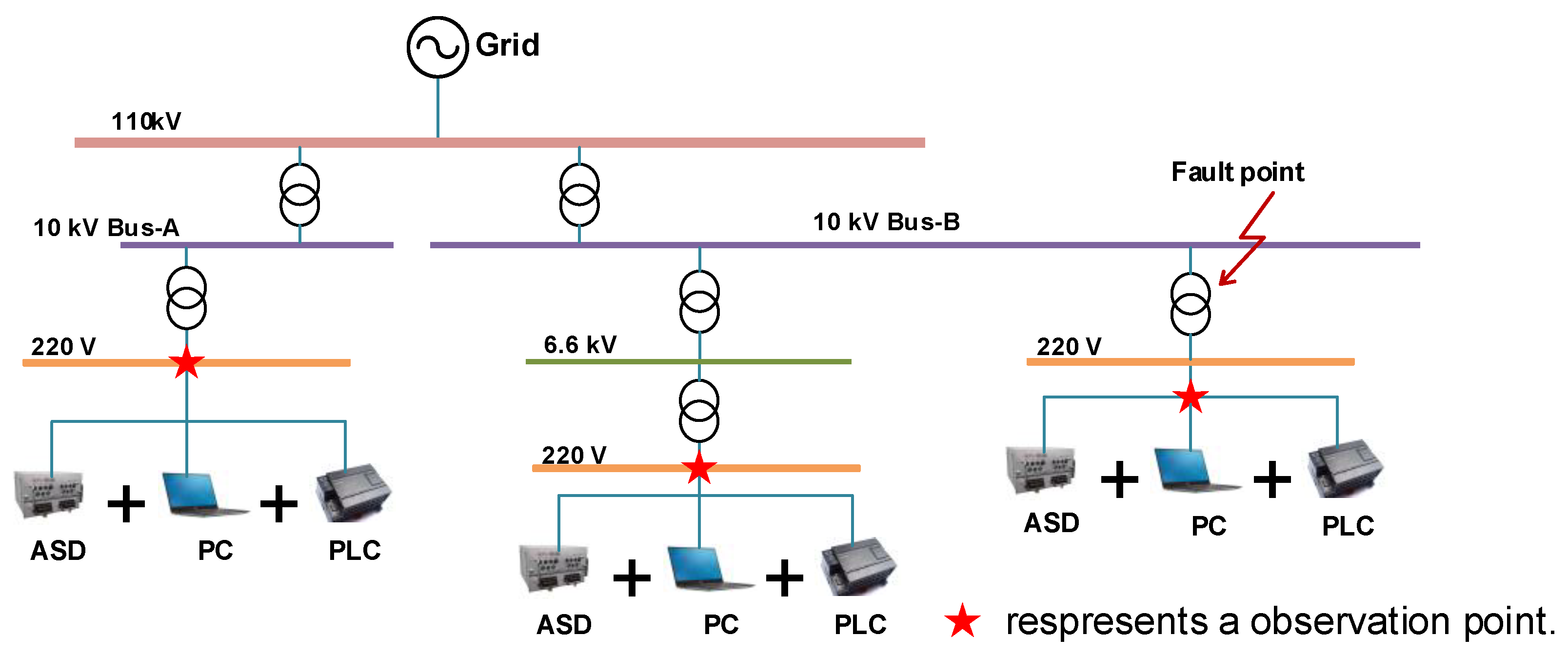
In accordance with the proposed method, the industrial distribution network model in PowerFactory is used for the simulations. As shown in Figure 5, the system voltage levels are 110 kV, 10 kV, and 6.6 kV. Three observation points are established in the figure, and it is assumed that each observation point is set with three types of sensitive equipment. The three types of sensitive equipment are selected based on the industrial distribution network, including a PLC (programmable logic controller), an ASD (adjustable speed device), and a PC (personal computer). Voltage amplitude and voltage duration limit values of the three typical sensitive equipment types are shown in

Table 3. Sensitive equipment’s voltage and duration limits.

Equipment Type	Umax (pu)	Umin (pu)	Tmax/ms	Tmin/ms
PLC	0.90	0.30	400	20
ASD	0.71	0.59	175	15
PC	0.63	0.46	205	40

[23,24,25,26].

At the fault point, three types of fault simulations, including single-phase short fault (SPSF), two-phase short fault (TPSF), and three-phase short fault (THPSF), are performed, respectively. Based on Appendix A, the specific values of five indexes on the source, network, and load side are calculated. The calculation results are shown in

Table 4. Index value of SPSF.

Observation Point	η/%	ΔE/J × 103	MSI	DSI	EIC
PLC of 10 kV bus-B	57.18	1.8448	35.3833	30.7105	0.6246
ASD of 10 kV bus-B	57.18	1.8448	18.5833	76.0625	0.6246
PC of 10 kV bus-B	57.18	1.8448	0	58.6061	0.6246
PLC of 10 kV bus-A	57.20	9.5185	35.4833	33.3421	0.6258
ASD of 10 kV bus-A	57.20	9.5185	19.0833	82.3125	0.6258
PC of 10 kV bus-A	57.20	9.5185	0	64.6667	0.6258
PLC of 6.6 kV bus	65.60	0.0229	17.8833	1.7632	0.2073
ASD of 6.6 kV bus	65.60	0.0229	0	7.3125	0.2073
PC of 6.6 kV bus	65.60	0.0229	0	0	0.2073

,

Table 5. Index value of TPSF.

Observation Point	η/%	ΔE/J × 103	MSI	DSI	EIC
PLC of 10 kV bus-B	50.33	2.1399	56.4670	43.8680	0.8776
ASD of 10 kV bus-B	50.33	2.1399	100	100	0.8776
PC of 10 kV bus-B	50.33	2.1399	40.4710	88.9090	0.8776
PLC of 10 kV bus-A	50.35	11.0409	56.5333	49.1316	1.4640
ASD of 10 kV bus-A	50.35	11.0409	100	100	1.4640
PC of 10 kV bus-A	50.35	11.0409	40.7059	100	1.4640
PLC of 6.6 kV bus	56.30	0.0291	33.2500	9.6579	0.5990
ASD of 6.6 kV bus	56.30	0.0291	7.9167	26.0625	0.5990
PC of 6.6 kV bus	56.30	0.0291	0	10.1212	0.5990

and

Table 6. Index value of THPSF.

Observation Point	η/%	ΔE/J × 103	MSI	DSI	EIC
PLC of 10 kV bus-B	50.33	2.1399	56.4670	43.8680	0.8776
ASD of 10 kV bus-B	50.33	2.1399	100	100	0.8776
PC of 10 kV bus-B	50.33	2.1399	40.4710	88.9090	0.8776
PLC of 10 kV bus-A	50.35	11.0409	56.5333	49.1316	1.464
ASD of 10 kV bus-A	50.35	11.0409	100	100	1.464
PC of 10 kV bus-A	50.35	11.0409	40.7059	100	1.464
PLC of 6.6 kV bus	56.30	0.0291	33.2500	9.6579	0.599
ASD of 6.6 kV bus	56.30	0.0291	7.9167	26.0625	0.599
PC of 6.6 kV bus	56.30	0.0291	0	10.1212	0.599

.

In view of the calculated indexes, the judgmental weights corresponding to each index are calculated through the method of maximizing deviation. The judgmental weights are as follows

Table 7. Judgmental weight of SPSF.

Index Category	η	ΔE	MSI	DSI	EIC
Weight	0.0210	0.2446	0.2927	0.2876	0.1541

,

Table 8. Judgmental weight of TPSF.

Index Category	η	ΔE	MSI	DSI	EIC
Weight	0.0179	0.3183	0.2626	0.2671	0.1341

and

Table 9. Judgmental weight of THPSF.

Index Category	η	ΔE	MSI	DSI	EIC
Weight	0.2133	0.4000	0.0429	0.1799	0.1639

:

The values of judgment weights can be substituted into Table 1, so that three judgment matrices for three fault types can be obtained. The judgment matrix under different fault types is substituted into Equation (15) to obtain the information entropy, which is listed in order according to SPSF, TPSF and THPSF: e_j = [0.7026, 0.2101, 0.1317, 0.1317, 0.4318], e_j = [0.7428, 0.1066, 0.1720, 0.1720, 0.4645] and e_j = [0.2404, 0.1761, 0.5810, 0.3114, 0.3114]. The entropy weight calculated by Equation (16) is given in the same order as above: a_j = [0.0877, 0.2329, 0.2560, 0.2560, 0.1675], a_j = [0.0770, 0.2673, 0.2477, 0.2477, 0.1602] and a_j = [0.2248, 0.2438, 0.1240, 0.2037, 0.2037].

Two different methods are used to calculate the weight of each index based on the judgmental matrix: one is AHP, and the other is CWM. The weight value selected by AHP does not change with the fault type. However, CWM carries out a weight calculation for each type of fault, while the weight value changes with the actual data. The following table lists the weight values calculated by the two referenced methods.

By linearly weighting the weight values obtained by the two methods in

Table 10. Index weight.

Index Category	AHP Weight	Comprehensive Weight (SPSF)	Comprehensive Weight (TPSF)	Comprehensive Weight (THPSF)
η	0.0301	0.0101	0.0086	0.1135
ΔE	0.1967	0.2050	0.4433	0.7475
MSI	0.3473	0.3657	0.2534	0.0116
DSI	0.3473	0.3657	0.2534	0.0637
EIC	0.0786	0.0535	0.0413	0.0637

and the corresponding coefficients in the superiority degree matrix, the corresponding evaluation values of voltage sag severity can be obtained.

In Figure 6, Figure 7 and Figure 8, the severity evaluation values calculated by AHP and CWM for SPSF and TPSP are found to have little difference, while the severity evaluation values calculated by the two methods for THPSF have a greater difference. This is because, when the comprehensive weight method is adopted, the dynamic changes of index data are considered for weight allocation, and each fault type is weighted once. The comprehensive weight method improves the rationality of the index weight.

In order to effectively assess the vulnerability of sensitive equipment when a voltage sag occurs, SPSF, TPSF, and THPSF are considered in the simulation. In each fault type, the severity level of the equipment on the 6.6 kV bus is Level 1 or Level 2. The equipment, when under these two levels, is relatively safe, and the voltage sag has little impact on the equipment. On the contrary, if the sensitive equipment on the 10 kV bus-A is Level 4 or Level 5 for each fault type, voltage sag will have a greater impact on equipment and if it is not managed, it will cause equipment damage and economic losses. Under SPSF and TPSF, the ASD and PLC of 10 kV bus-B are of a high severity level and may cause damage to the equipment.

5. Conclusions

In this paper, a comprehensive index system that integrates multi-side indexes of the source, the network, and the load using the comprehensive weight method to evaluate the voltage sag severity, is presented. The main contributions of this article are as follows:

(1)

The proposed multi-side index system has the ability to reduce the potential of the evaluation level of voltage sag severity being overestimated, as can happen when only the load index is considered.

(2)

The comprehensive weighting method, by combining the merits of the entropy weight method and IAHP, is proposed to give consideration to both subjective and objective evaluation.

(3)

The vulnerability of sensitive equipment under different voltage sag conditions was comprehensively and concretely evaluated by the case studies of different types of circuit faults in the distribution network.

References

1. Liu, J.H.; Chen, K.X.; Ma, J.; Xu, C.H.; Wu, J.H. Classification of three-phase voltage dips based on CNN and random forest. Power Syst. Prot. Control 2019, 47, 112–118. [Google Scholar]
2. Li, Z.M.; Li, W.W.; Pan, T.H. An optimized compensation strategy of DVR for micro-grid voltage sag. Prot. Control Mod. Power Syst. 2016, 1, 10. [Google Scholar] [CrossRef] [Green Version]
3. Li, S.; Jiang, C.C.; Zhao, Z.Y.; Li, Z.Y. Study of transient voltage stability for distributed photovoltaic power plant integration into low voltage distribution network. Power Syst. Prot. Control 2017, 45, 67–72. [Google Scholar]
4. Amir, S.; Mahmud, F.; Matti, L. A General Framework for Voltage Sag Performance Analysis of Distribution Networks. Energies 2019, 12, 2824. [Google Scholar]
5. Motoki, E.; Filho, J.; da Silveira, P.; Pereira, N.; de Souza, P. Cost of Industrial Process Shutdowns Due to Voltage Sag and Short Interruption. Energies 2021, 14, 2874. [Google Scholar] [CrossRef]
6. Liu, Q.Y.; Liu, F.; Zou, R.M.; Li, Y. Harmonic Resonance Characteristic of Large-scale PV Plant: Modelling, Analysis and Engineering Case. IEEE Trans. Power Deliv. 2021, 30, 2392–2400. [Google Scholar]
7. Bollen, M.H.J.; Sabin, D.D. International coordination for voltage sag indices. In Proceedings of the IEEE Power Engineering Society Transmission and Distribution Conference, San Francisco, CA, USA, 21–24 May 2006; IEEE: New York, NY, USA, 2006; pp. 229–234. [Google Scholar]
8. Chan, J.Y.; Milanovic, J.V. Severity Indices for Assessment of Equipment Sensitivity to Voltage Sags and Short Interruptions. In Proceedings of the 2007 IEEE Power Engineering Society General Meeting, Tampa, FL, USA, 24–28 June 2007; IEEE: New York, NY, USA, 2007; pp. 1–7. [Google Scholar]
9. Wang, Y.; Dong, Y. Evaluation of voltage sag severity based on multisource causative attribute. In Proceedings of the 2019 IEEE Sustainable Power and Energy Conference (ISPEC), Beijing, China, 21–23 November 2019; IEEE: New York, NY, USA, 2020; pp. 815–820. [Google Scholar]
10. Yang, J.L.; Xu, Y.H. Comprehensive evaluation method of node voltage sag severity based on TOPSIS model and combination weights. Power Syst. Prot. Control 2017, 45, 88–95. [Google Scholar]
11. Zeng, J.; Cai, D.Y. A monte carlo assessment method of voltage sags based on combination weight. Power Syst. Technol. 2016, 40, 1469–1475. [Google Scholar]
12. Xu, Y.H.; Fan, X.G.; Deng, S.Y.; Niu, C.H. A Voltage Sag Severity Evaluation Method for the System Side Which Considers the Influence of the Voltage Tolerance Curve and Sag Type. Energies 2021, 14, 5065. [Google Scholar] [CrossRef]
13. Zhou, X.; Wang, F.H.; Zhang, J.; Huang, R.H. A voltage sag severity index considering the power system and consumer equipment. In Proceedings of the 2014 IEEE PES General Conference & Exposition, National Harbor, MD, USA, 27–31 July 2014; IEEE: New York, NY, USA, 2014; pp. 1–5. [Google Scholar]
14. Pan, L.; Zhang, P.; Yu, X. Comprehensive Evaluation of Node Voltage Sag Severity Considering the Power Grid Side and the User Side. In Proceedings of the 2018 China International Conference on Electricity Distribution (CICED), Tianjin, China, 17–19 September 2018; IEEE: New York, NY, USA, 2018; pp. 467–471. [Google Scholar]
15. Wu, G.; Zhong, Q.; He, Q.; Xu, Z. Evaluation Method and Probabilistic Index of Voltage Sag Severity Considering Point-on-wave. J. Mod. Power Syst. Clean Energy 2021, 9, 633–638. [Google Scholar]
16. Chang, H.Y.P.; Gilsoo, J. Systematic Method to Identify an Area of Vulnerability to Voltage Sags. IEEE Trans. Power Deliv. 2017, 32, 1583–1591. [Google Scholar]
17. Liao, H.; Abdelrahman, S.; Guo, Y.; Milanovic, J. Identification of Weak Areas of Power Network Based on Exposure to Voltage Sags—Part I: Development of Sag Severity Index for Single-Event Characterization. IEEE Trans. Power Deliv. 2015, 30, 2392–2400. [Google Scholar] [CrossRef]
18. Biswas, S.; Goswami, S.K.; Chatterjee, A. Optimum distributed generation placement with voltage sag effect minimization. Energy Convers. Manag. 2012, 53, 163–174. [Google Scholar] [CrossRef]
19. Xiao, X.Y.; Chen, W.D.; Yang, H.G.; Li, H.Q. Voltage Sag Frequency Assessment under the Measure of Interval Data of Customer Satisfaction. Proc. CSEE 2010, 30, 104–110. [Google Scholar]
20. Djokic, S.Z.; Desmet, J.; Vanalme, G.; Milanovic, J.V.; Stockman, K. Sensitivity of personal computers to voltage sags and short interruptions. IEEE Trans. Power Deliv. 2005, 20, 375–383. [Google Scholar] [CrossRef]
21. Djokic, S.Z.; Stockman, K.; Milanovic, J.V.; Desmet, J.J.M.; Belmans, R. Sensitivity of AC adjustable speed drives to voltage sags and short interruptions. IEEE Trans. Power Deliv. 2005, 20, 494–505. [Google Scholar]
22. Gupta, C.P.; Milanovic, J.V. Probabilistic assessment of equipment trips due to voltage sags. IEEE Trans. Power Deliv. 2006, 21, 711–718. [Google Scholar] [CrossRef]
23. Kong, F.; Liu, H.Y. A new fuzzy MADM algorithm based on subjective and objective integrated weights. In Proceedings of the 2007 International Conference on Service Management, Chengdu, China, 9–11 June 2007; IEEE: New York, NY, USA, 2007; pp. 1–6. [Google Scholar]
24. Wu, Y.; Li, C.; Xu, Y.; Wei, P. Characterizing the tolerance performance of PLCs to voltage sag based on experimental research. In Proceedings of the 2016 IEEE PES Asia-Pacific Power and Energy Engineering Conference (APPEEC), Xi’an, China, 25–28 October 2016; pp. 496–501. [Google Scholar]
25. Escribano, A.H.; Gómez-Lázaro, E.; Molina-García, A.; Fuentes, J. Influence of voltage dips on industrial equipment: Analysis and assessment. Int. J. Electr. Power Energy Syst. 2012, 41, 87–95. [Google Scholar] [CrossRef]
26. Djokic, S.; Milanovic, J.; Kirschen, D. Sensitivity of AC Coil Contactors to Voltage Sags, Short Interruptions, and Undervoltage Transients. IEEE Trans. Power Deliv. 2004, 19, 1299–1307. [Google Scholar] [CrossRef]
Figure 1. Voltage sag severity index system.
Energies 14 06434 g001
Figure 2. Sensitive equipment SEMI F47 curve.
Energies 14 06434 g002
Figure 3. Flow chart of superiority matrix construction.
Energies 14 06434 g003
Figure 4. Flow chart of voltage sag severity calculation.
Energies 14 06434 g004
Figure 5. Industrial distribution network.
Energies 14 06434 g005
Figure 6. Voltage sag severity level of SPSF.
Energies 14 06434 g006
Figure 7. Voltage sag severity level of TPSF.
Energies 14 06434 g007
Figure 8. Voltage sag severity level of THPSF.
Energies 14 06434 g008