Numerical Analysis and Parameter Optimization of J-Shaped Blade on Offshore Vertical Axis Wind Turbine

Abstract

In this study, the performance of offshore wind turbines at low tip speed ratio (TSR) is studied using computational fluid dynamics (CFD), and the performance of offshore wind turbines at low tip speed ratio (TSR) is improved by revising the blade structure. First, the parameters of vertical axis offshore wind turbine are designed based on the compactness iteration, a CFD simulation model is established, and the turbulence model is selected through simulation analysis to verify the independence of grid and time step. Compared with previous experimental results, it is shown that the two-dimensional simulation only considers the plane turbulence effect, and the simulation turbulence effect performs more obviously at a high tip ratio, while the three-dimensional simulation turbulence effect has well-fitting performance at high tip ratio. Second, a J-shaped blade with optimized lower surface is proposed. The study showed that the optimized J-shaped blade significantly improved its upwind torque and wind energy capture rate. Finally, the performance of the optimized J-blade offshore wind turbine is analyzed.

1. Introduction

Global warming and rising sea levels have made the search for renewable energy more urgent [1]. Europe is rich in wind energy, among several common renewable energy sources; it has been a good renewable energy source and is now one of the fastest growing renewable energy sources in the world [2,3]. Offshore wind turbines can be divided into two categories: offshore horizontal axis wind turbine (HAWT) and offshore vertical axis wind turbine (VAWT). Due to the high efficiency of the wind energy of horizontal axis offshore wind turbine, most large-scale wind power generation is now based on the horizontal axis [4,5,6]. Due to the high utilization rate of wind energy and mature technology of large-scale horizontal axis offshore wind turbines, large-scale wind power generation is now mostly horizontal axis, which occupies a large share in both offshore wind power and onshore wind power [7,8]. While the larger size of the offshore wind turbine helps reduce the cost of generating electricity, it also significantly increases the cost of operation and maintenance, especially for offshore wind turbines that require installation and maintenance on specific vessels [9,10]. With the increase of the size of offshore wind turbines, the cost of power generation is reduced, which also brings difficulties to the construction and maintenance of large-scale offshore wind turbines [11]. On the contrary, since the generator and gearbox system of the vertical axis offshore wind turbine is installed on the base, the theoretical limit of the top rotor can reach 30MW, so increasing the size of the vertical axis offshore wind turbine does not bring many negative effects [12]. As we can see from Figure 1, the offshore floating vertical axis offshore wind turbines are running on the surface of the deep ocean.

The improvement of blade structure has always been an important direction of offshore wind turbine research. By changing the blade shape, the vertical axis offshore wind turbine can adapt to different working conditions and improve the torque performance and wind energy capture rate of offshore wind turbine. The experimental design and CFD simulation were carried out on the vertical axis offshore wind turbine. The optimization variable of small wings can be reduced by keeping the pressure difference on both sides of the blade tip vortex, which can improve the power factor. The power output and the improvement of the wings on the vertical axis offshore wind turbine mainly be changed in the direction of the offshore wind [14]. Sobhani E. et al. established a cavity on the blade of VAWT and changed the flow field around the blade. The results showed that the circular fin with a diameter of 8% chord length was the best near the pressure side and leading edge of the airfoil [10]. Compared with the reference airfoil, the wind energy capture rate of the wind generator with a cavity was improved by 18% at $\mathrm{TSR}=2.6$. Mohamed O.S. et al. studied the startup performance of a vertical axis offshore wind turbine with slotted airfoil blades and optimized the slotted position, inclination, and size. The results showed that at large angles of attack, the torque and power coefficient at low tip speed ratio could be improved by delayed eddy current separation [15].

Zamani M. et al. proposed a J-shaped blade with trailing edge opening on the lower surface of the blade, indicating that the J-shaped blade can optimize the performance of the wind generator, eliminate the pressure surface at the maximum thickness of the trailing edge of the airfoil, and improve the self-starting ability of the wind generator [16]. In addition, J-shaped blades with openings on the upper surface are proposed to generate both lift and drag forces. This combined force helps the turbine to operate faster at low wind speeds, especially at low tip speed ratio, which improves self-starting and wind energy capture [17]. M.H. Mohamed et al. analyzed three types of offshore wind turbines with different airfoil sections, and compared the performance and noise of J-blade offshore wind turbines [18].

The above study is feasible for ascension offshore wind turbine blade structure to improve performance. The 2-D simulation of the offshore wind turbine J-shape blade did not consider the performance of the low wind speed. At the same time, surface changes of offshore wind turbine J-shape blade have some shortcomings on performance impact. Thus, in this study, the J-shape blade structure has been improved. Therefore, in this study, when the azimuth angle of J-shaped blade is between 60° and 180°, the torque is improved through resistance, and the influence of the change of the upper surface on the performance of the wind generator is analyzed. By analyzing the change curve of instantaneous blade torque, it is found that when the blade tip speed ratio is low, the azimuth angle between 60° and 180° will produce negative torque. The results show that both the torque and the wind energy capture rate increase when the blade tip speed ratio is low. Then, the flow field of the J-shaped blade is analyzed, and it is found that the resistance of the lower surface of the blade is larger when the azimuth angle is between 60° and 90°. Compared with the symmetrical airfoil offshore wind turbine, both the torque and the wind energy capture rate are improved at low tip speed ratio. When the wind speed is 9 m/s and TSR = 1, the average torque of the wind generator is 64.05. Based on the above studies, they mainly focus on the influence of characteristic parameters on the wind energy capture rate. There are many studies on the starting torque and wind energy capture rate of the hybrid vertical axis offshore wind turbine of Savonius and Darrieus; thus, it is difficult to install the hybrid vertical axis offshore wind turbine, and Savonius will reduce the wind energy capture rate when the blade tip ratio is high. The proposed J-blade and the optimized J-blade are based on the NACA0018 blade to adopt a single vertical axis offshore wind turbine and to improve the self-starting capacity such that a good wind energy capture rate can be obtained at a low tip speed ratio.

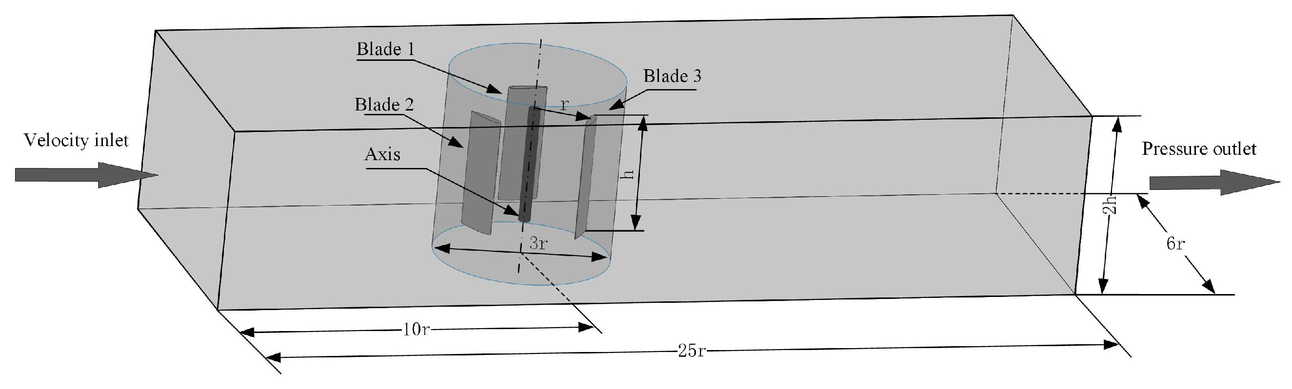
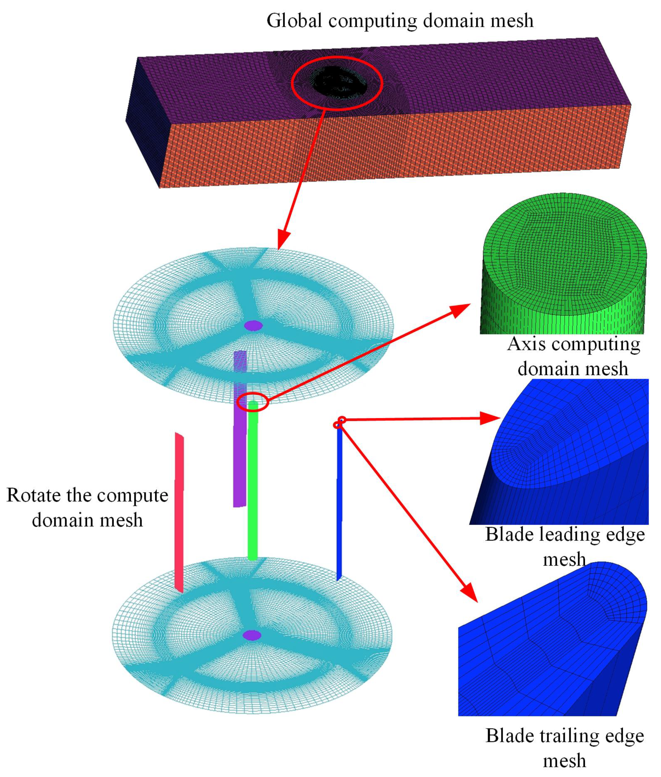
The rest of this study is outlined as follows. First, in Section 2, we introduce the parameters of the design of vertical axis offshore wind turbines. In Section 3, we present CFD simulation modeling technology on vertical axis offshore wind turbines, such as the physical model, turbulence model, computational domain, and meshing. In Section 4, the results and discussion of the vertical axis offshore wind turbine torque and wind energy capture rate, torque coefficient, velocity, and pressure cloud maps are analyzed. We conclude the study in Section 6.

2. Parameters of the Design of Vertical Axis Offshore Wind Turbines

In the design of vertical axis offshore wind turbine, if the aspect ratio of offshore wind turbine is not chosen properly, the power coefficient of offshore wind turbine will be low. The design parameters are usually selected according to the experience of the designer. In the design process of offshore wind turbines, curves of power coefficients of different compactness changing with blade tip speed ratio need to be drawn to establish the relationship between aspect ratio and offshore wind turbine performance [19,20]. 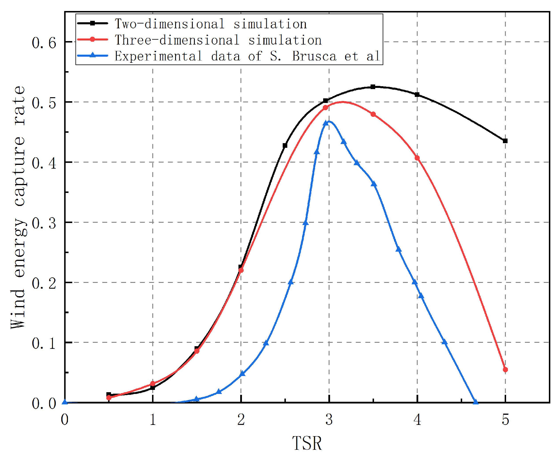The results show the change curve of wind energy capture rate with tip velocity ratio when the Reynolds number of the NACA0018 airfoil wind generator is selected with $5\times 10^6$, $1\times 10^6$, $3.6\times 10^5$, and $1.6\times 10^5$, and compactness is selected with 0.75, 0.5, 0.4, 0.3, 0.2, and 0.1, respectively. It can be seen that the maximum wind capture rate increases with the increase of Reynolds number, and the corresponding tip speed ratio decreases. This study adopts the design process of S. Brusca et al. [19]. Based on the compactness, the three-blade vertical blade wind generator is designed. One computes the maximum energy capture rate of the wind generator, as well as the corresponding blade tip speed ratio, which are shown in Figure 2.

The study shows the change curve of wind energy capture rate with blade tip speed ratio under different compactness with Reynolds number $Re=5\times {10}^6$. It can be seen when the compactness $\sigma =0.3$ that the maximum wind energy capture rate of the wind generator $C{p}_{max}=0.51$ and the corresponding blade tip speed ratio ${\lambda }_{Cpmax}=3.0$. Where the compactness can be changed by the number of blades, chord length, and rotation radius, reflecting the proportion of blades in the sweep surface. The curve of wind energy capture rate corresponding to low compactness is relatively smooth. When the blade tip speed ratio changes in a wide window, the range of wind energy capture rate changes is small, but it increases the resistance to wind, so the maximum wind energy capture rate is small. Under high compactness, the wind energy utilization curve is sharper, the maximum wind energy capture rate is larger, and it is more sensitive to the change of tip velocity ratio. If the compactness is too large, the maximum wind capture rate has a relatively low maximum value, and the decrease in the maximum wind capture rate is caused by the stall loss. The compactness is expressed by Equation (1):

$$\sigma =\frac{Nc}{r}$$

(1)

Here, N is the number of offshore wind turbine blades. r is rotate radius. The function of blade chord length can be expressed by the description of compactness c. c is shown by the following Equation (2):

$$c=\frac{r{\sigma }_{C_{p}max}}{N}$$

(2)

In the formula, ${\sigma }_{C_{p}max}$ is the corresponding compactness when the offshore wind turbine obtains the maximum wind energy capture rate. The actual power of the offshore wind turbine is expressed by Equation (3):

$$P=\frac{1}{2}\rho V_{\infty }^{3}2rh{C}_p$$

(3)

Here, $C_p$ is the wind energy utilization factor. The horizontal axis offshore wind turbine aspect ratio is defined as the ratio of leaf length and leaf chord length. In this study, the vertical axis offshore wind turbines aspect ratio $R_z$ is defined as the ratio of offshore wind turbine blade height h and rotate radius r. The radius of rotation is inversely proportional to the height of the blade. In the initial design, the offshore wind turbine has a relatively small aspect chord, which is aimed for minimize the blade height and shaft diameter for a given sweep area. When the blade tip speed ratio is fixed, if the aspect ratio is increased, the rotor speed will increase; if the power is constant, the torque will decrease. The aspect ratio is expressed by Equation (4):

$$R_z=\frac{h}{r}$$

(4)

According to Equations (3) and (4), the rotating radius of offshore wind turbine blade can be expressed as Equation (5):

$$r=\sqrt{\frac{P}{\rho V_{\infty }^3{R}_{z}Cp}}$$

(5)

Here, P is described in Equation (3). In iterative design, the Reynolds number of the blade needs to be recalculated. The actual Reynolds number is expressed by Equation (6):

$$Re=\frac{cW}{\nu }$$

(6)

Here, W is relative wind speed of blades. In the formula, $\nu$ is the kinematic viscosity of air. Blade tip speed ratio $\lambda$ is the ratio of the linear velocity of blade rotation around the spindle to the incoming wind speed, reflecting the relative speed of the wind generator, which can be expressed by Equation (7). When the vertical axis offshore wind turbine is running at high tip ratio, the centrifugal force on the blade is large, which requires high structural strength of the offshore wind turbine.

$$\lambda =\frac{V}{V_{\infty }}=\frac{\omega r}{V_{\infty }}$$

(7)

Using mathematical approximation method, the relative wind speed W can be replaced by the blade tip speed $V=Wr$ and transformed into the mean Reynolds number independent of azimuth angle $\theta$. Equations (6) and (7) can derive Equation (8) of average Reynolds number:

$$Re=\frac{c{V}_{\infty }{\lambda }_{Cpmax}}{\nu }$$

(8)

In the formula, $C{p}_{max}$ is the blade tip speed ratio corresponding to the maximum wind energy capture rate of the wind generator.

The iterative design process of the offshore wind turbine is shown in Figure 3. In design, only four parameters, namely rated power P of offshore wind turbine, number of blades N, inlet wind speed $V_{\infty }$, and aspect ratio of offshore wind turbine $R_z$, need to be known. In the literature [19], the wind energy capture rate curve corresponding to the Reynolds number of the initial test is selected first; then, the corresponding ${\sigma }_{Cpmax}$ and ${\lambda }_{Cpmax}$ when the wind power generator obtains the maximum wind energy capture rate $C{p}_{max}$ are found. The radius, chord length, and Reynolds number of the wind power generator are calculated using Equations (2), (5), and (8), respectively. As the Reynolds number changes with the main size of the turbine rotor, the rotor diameter increases and the blade tip speed increases, resulting in the Reynolds number increasing. Therefore, the power coefficient of the offshore wind turbine generator is greatly affected, and it is necessary to calculate the Reynolds number and the Reynolds error of the initial test. If the calculation of the Reynolds number and the initial error using the power coefficient curve of Reynolds number requires one to draw a new Reynolds number or use a Reynolds number wind energy curve similar to the second iteration, ignore the Reynolds number effects on the performance of offshore wind turbine, if the error iteration of the offshore wind turbine parameters is designed for offshore wind turbines. Typically, the iterative design process takes only two or three iterations.

The wind generator is designed according to Figure 2, and the iterative design parameters are shown in

Table 1. Offshore wind turbine design iteration parameters.

Parameter	References	First Iteration	Second Iteration
Rated power	-	2.7 kw	2.7 kw
Airfoil	-	NACA0018	NACA0018
Air density	-	1.2 kg/m${}^3$	1.2 kg/m${}^3$
Viscosity	-	$1.46\times {10}^{-6}$ m${}^2$/s	$1.46\times {10}^{-6}$ m${}^2$/s
Wind speed	-	12 m/s	12 m/s
Aspect ratio	-	2	2
Number of blades	-	3	3
Trial Reynolds	-	$5.0\times {10}^6$	$2.4\times {10}^5$
$C{p}_{max},{\sigma }_{Cpmax},{\lambda }_{Cpmax}$	[19]	0.51; 0.3; 3.0	0.464; 0.4; 2.96
The rotor radius	Formula (5)	0.972 m	1.019 m
Blade chord	Formula (2)	0.0972 m	0.13568 m
Second try Reynolds number	Formula (8)	$2.4\times {10}^5$	$3.3\times {10}^5$
The next step	-	The second attempt	End of the iteration

. Assuming that the design airfoil is NACA0018, the design parameters of the vertical axis offshore wind turbine are as follows: rated power P = 2.7 kw, blade number $N=3$, design wind speed $V_{\infty }$ = 12 m/s, and aspect ratio $R_z=2$.

3. CFD Simulation Modeling Technology

3.1. Physical Model

In order to facilitate modeling, the design parameters of offshore wind turbine are modified. The chord length of the blade is c = 0.136 m, the radius of the offshore wind turbine is r = 1 m, and the height of the offshore wind turbine blade h = 2 m can be obtained from aspect ratio and rotation radius, as shown in

Table 2. Wind generator parameters.

Parameter	Specific Numerical
Rated power	2.7 kw
Blade airfoil	NACA0018
Number of blades	3
Axis diameter	0.1 m
Wind speed	12 m${}^2$/s
Blade and shaft height	2 m
Blade chord	0.136 m
Radius	1 m

:

Figure 4 shows a simplified front vertical axis offshore wind turbine with J-shaped blades. Except that the blades are changed into J-shaped blades, the other parameters are the same; ignoring the influence of connecting arms, the length of the main shaft and the height of the blades are the same. The offshore wind turbine outflow field simulation analysis must first establish the offshore wind turbine model, according to the revised design parameters to establish a three-dimensional model in SolidWorks. A model of a symmetrical airfoil vertical axis wind generator is shown in Figure 4. The structure of a vertical axis wind generator includes blades, main axes, supporting arms, and flanges. The rotation axis and the blade are perpendicular to the horizontal plane, and the flow field around the spindle rotates around the center is the flow around a cylinder, which is also affected by the wake flow when the blade rotates around a fixed radius of the spindle. The upper support arm and the lower support arm are parallel to the horizontal plane. Small windward side has little influence on the flow field around the wind generator. In order to facilitate mesh division, the influence of the spindle is considered to ignore the influence of the support arm, and the height of the spindle is simplified to the height of the blade. Then, the model is derived to divide the computing domain and mesh in ANSYS ICEM.

We choose a symmetrical improved J-shape blade of airfoil NACA0018 as an example. The J-shape of blade is divided into two symmetrical parts. Through the surface along the chord length direction, adjusting the leading edge of the distance and J-shape on the blade surface size, it can be seen that the J type blade is small comparing to the traditional symmetrical blade surface. There is a gap on the blade surface that is similar to the resistance type blades of offshore wind turbine. When the azimuth is in the interval of [60°,180°], we provide greater torque for the wind generator, and the blade can provide torque for the wind generator through lift force when it is in the downwind direction, which is shown in Figure 5.

Figure 6 shows the influence of structural changes of J-shaped blades on offshore wind turbine performance. The aerodynamic performance of NACA0018 0.05c, NACA0018 0.1c, NACA0018 0.15c, NACA0018 0.25c, and NACA0018 0.25cnew blades is analyzed. c is the chord length of the blade, the offshore wind turbine with different number models(0.1c, 0.25c, 0.25c) indicate different chord lengths of the blade. Take the 0.15c blade of NACA0018 as an example, where 0.15c is the distance between the upper surface of the blade and the leading edge along the chord direction. NACA0018 0.15cnew is a J-shaped blade optimized on the lower surface. The upper surface of NACA0018 0.15cnew is the same as NACA 00180.15c, the lower surface is a horizontal tangent of the blade, the chord length of the blade is 136 mm, and the thickness is 2 mm. By comparing the simulation analysis of J-shaped blade with the symmetric airfoil NACA0018, the influence of the upper surface change and the lower surface change on the wind energy capture rate and the torque is analyzed. The NACA0018 0.25cnew and NACA0018 0.15cnew blades have a better performance than the original NACA0018 0.25c and NACA0018 0.15c on wind energy capture rate and the torque, respectively.

3.2. Computational Domain

The selection of calculation domain parameters will affect the simulation results of offshore wind turbines [21,22]. When the outflow field of offshore wind turbine is simulated, the calculation field should be infinite. However, the calculation cost is considered in the actual simulation. Because the influence of the outflow field on the offshore wind turbine is reduced when it is far away from the offshore wind turbine, the influence on the performance of the offshore wind turbine can be ignored by selecting the appropriate size parameters of the calculation field. The whole simulation computing domain is a cuboid, and the wind generator is located near the entrance. It is composed of the stationary domain and the rotating domain, which is a multireference domain model. Although the sliding grid model can only carry out transient calculation and requires a lot of calculation time, the stationary and rotating domains interact with each other in the process of wind generator simulation, so the sliding grid model can better capture transient flows [7,23].

Figure 7 and Figure 8 are two-dimensional and three-dimensional computing domain models. In order to keep the wind speed flowing into the computing domain stable and prevent the wind speed change from affecting the flow field around the wind generator, a certain distance should be reserved from the wind generator entrance. Similarly, in order to observe the surrounding conditions of the wind generator and the wake conditions, and to consider the turbulence caused by the wind passing through the wind generator, the backflow outlet also needs to have a certain distance from the wind generator. We analyze the research on the division of the computing domain of offshore wind turbines. The computing domain dimensions are set as follows: the inlet boundary of the rotating main wheelbase of offshore wind turbines is $10r$, and the exit boundary is $15r$; the diameter of the rotation domain is $3r$, where r is the rotation radius of the offshore wind turbine; the height of the blade and spindle of the offshore wind turbine is h, and the height of the calculation domain is $2h$.

3.3. Mesh Generation and Independent Validation

Figure 9 show the three-dimensional grid of the wind generator, which is composed of the static domain grid and the rotating domain grid. In order to facilitate grid division, the rotating domain grid includes the rotating domain grid around the blade and the rotating domain grid around the spindle. Grid structure theoretically and unstructured grid can be used for offshore wind turbine fluid simulation grid, but in this article, we mainly focus on improvement of leaf tissue structure to maintain the stability of a grid that is easy to transplant. At the same time, considering the blade viscous boundary layer effect on offshore wind turbine simulation results, and the need to study the flow field around the offshore wind turbine blade, the grid division is adopted. ANSYS ICEM software is used to divide the grid, and the whole grid consisted of three parts: static field grid, blade rotation field grid, and spindle rotation field grid. The grid of the stationary region is sparse in secondary regions, whereas the grid of the spindle rotation domain and the grid of the blade rotation domain are dense in the moving region of the wind generator. Such grid division not only reduces the calculation time but also effectively improves the calculation accuracy.

ANSYS ICEM is still used to divide the grid according to the computing domain, the stationary domain grid is sparse, and the rotating domain grid is dense. After the establishment of each computing domain grid, the grid is combined. In this way, the mesh density can be adjusted for different computing domains, and appropriate sliding mesh parameters can be set at the same time. The rotation speed of the rotating domain can be calculated by the blade tip speed ratio. The quadrilateral mesh is used for 2D simulation, and the hexahedral mesh is used for 3D simulation.

The grid quality in offshore wind turbine fluid simulation directly affects the simulation results. It is found that with the increase of grid density, the simulation accuracy gradually increases. If the grid density is too large, the accuracy can be improved, but a lot of computing time is wasted. If the grid accuracy is small, the calculation accuracy is too low. In order to analyze the influence of the number of grids used on the performance of the offshore wind turbine, the simplified offshore wind turbine model is divided into four grids as follows: Mesh 1, Mesh 2, Mesh 3, and Mesh 4, and the number of grids in each computing domain is shown in

Table 3. Number of Three-dimensional meshs.

Computational Domain	Mesh 1	Mesh 2	Mesh 3	Mesh 4
Stationary domain	190,800	412,160	590,240	718,000
Shaft rotation domain	135,680	426,480	528,720	682,240
Blade rotation domain	2,141,520	3,847,104	4,661,032	6,181,344
Total	2,468,000	4,685,744	5,779,992	7,581,584

. It can be seen from the table that the grids are mainly concentrated in the rotating domain, because the flow in the rotating domain is complex and the grid density in the main part of wind generator simulation is much higher than that in the stationary domain.

k-$\omega$ turbulence model is used in the simulation, with tip speed ratio TSR = 2.96 and wind speed of 12 m/s. The simulation results are shown in Figure 10. The wind energy capture rate of four grids with different densities is calculated, and the curve of wind energy capture rate changing with the grid density is drawn. When grid density increases from mesh 1 to mesh 2, the number of grids increases by $2.217744\times 10^6$ wind energy capture rate increases by $0.06$; when mesh 2 increases to mesh 4, the number of grids increases by $2.895840\times 10^6$ wind energy capture rate increases by $0.013$. The wind energy capture rate increases by 2.65% based on mesh 2, but the simulation time is doubled, and mesh 2 is adopted as the simulation mesh.

When dividing the wall layer grid, since the near wall is the main source of eddy currents, the wall will cause the turbulent momentum boundary layer. In order to accurately simulate the turbulence generation, the wall layer grid needs to be dense. The wall function method uses the empirical formula to estimate and process the viscous sublayer, and does not need the overdense boundary layer mesh, which can save the calculation time and achieve a higher accuracy. In this study, the wall function method is adopted to estimate the grid height $y$ of the first layer, and then it is judged whether $y^{+}$ meets the conditions according to the simulation results, which can be expressed by Equation (9):

$$y^{+}=\frac{\rho y{u}_{\tau }}{\mu }$$

(9)

In the formula, $y^{+}$ is the wall distance; y is the mesh height of the first layer; $u_{\tau }$ is the shear velocity of the near wall fluid.

Since the size of $y^{+}$ affects the node position of the first layer mesh, a dense mesh is required for solving the viscous sublayer. Different turbulence models have different requirements for $y^{+}$. k-$ϵ$ turbulence model requires a $y^{+}$ value around 30, while k-$ϵ$ turbulence model usually requires a $y^{+}$ value close to 1. In this study, the SST k-$\omega$ turbulence model is mainly used for simulation. As can be seen from Figure 11, the $y^{+}$ value on the spindle is closer to 1 and it is smaller at the blade. This is because the grid around the blade is denser with high linear velocity of the offshore wind turbine blade, and the maximum $y^{+}$ value of both the blade and the spindle is less than 1.2, which can meet the requirements of wall mesh.

Figure 12 shows the 2D and 3D mesh of the J-blade wind generator. Due to the time limitation of simulation, only the optimized J-blade on the lower surface is simulated in 3D. Figure 12a–d shows the 2D mesh of the blade when the distance between the upper surface and the leading edge along the string direction is 0.05C, 0.1C, 0.15C, and 0.25C, respectively. In order to facilitate the mesh division of the structure and meet the mesh accuracy requirements, O-shaped blocks are used to divide the blade, and C blocks are used to divide the mesh behind the trailing edge. Figure 12e–f shows the 2D and 3D grids after optimization of the lower surface of the blade, respectively. The turbulence intensity at the top and bottom of the blade is relatively high, so the grids at the top and bottom of the blade are dense.

Figure 13 shows the three-dimensional J-shaped blade modified on the lower surface and the $y^{+}$ distribution near the main axis. It can be seen from the figure that the maximum value of the wall $y^{+}$ is less than 3.2, the leading edge of the blade and the windward side wall of the main shaft have a large $y^{+}$ value around 1, and the leeward side wall has a $y^{+}$ value less than 1. Therefore, the wall grid can meet the requirements of the SST k-$\omega$ turbulence model for offshore wind turbine simulation.

3.4. Time Step Independence Verification

For offshore wind turbine simulation, using transient simulation results of the calculation of time step is another important factor; if the selected time step is too small, a large increase in computing time and large time step calculation precision is not enough, so choosing the appropriate time step for accuracy and computer numerical simulation results force balance is of great significance. Considering that the offshore wind turbine is a periodic rotating movement, the rotation angle of the offshore wind turbine per unit time step is 7.2°, 5°, and 4° for the convenience of later analysis to verify the influence of time step on the performance of the offshore wind turbine. It can be seen from

Table 4. Different blade tip speed ratio corresponds to the time step of each step.

TSR	Each Step 7.2°	Each Step 5°	Each Step 4°
0.5	0.0209	0.0145	0.0116
1	0.0105	0.0073	0.0085
1.5	0.0070	0.0048	0.0039
2	0.0052	0.0036	0.0029
2.5	0.0042	0.0029	0.0023
2.96	0.0035	0.0025	0.0020
3.5	0.0030	0.0021	0.0017
4	0.0026	0.0018	0.0015
5	0.0021	0.0015	0.0012

that the improved J-blade wind turbine has a lower tip speed ratio than a symmetrical wind turbine. Although the wind energy capture rate will decrease at high tip speed ratios, the wind energy capture rate has been greatly increased at low tip speed ratios.

Figure 14 shows that the torque curves of offshore wind turbines with rotation angles corresponding to the three time steps of 7.2°, 5°, and 4° have converged and presented periodic changes, and there are large torque differences near the low and high points of the torque curves. In general, the smaller the time step, the higher the calculation accuracy. Considering the calculation time and calculation accuracy, this study chooses the time step as the simulation time step.

3.5. Turbulence Model Analysis

It is complicated to solve the turbulent motion in computational fluid dynamics [24]. In the current calculation, one turbulence model cannot accurately describe all the turbulent motion or obtain the solution with sufficient precision. Therefore, the simulation results of offshore wind turbines with three different turbulence models are selected for analysis. The Spalart–Allmaras turbulence model is a single equation model mainly used in aerospace applications.Because the Spalart–Allmaras model does not calculate the turbulent kinetic energy, and the wind generator simulation needs to accurately simulate the rotating state of the wind generator, this model is not adopted. Both k-$\omega$ and K-$ϵ$ are widely used two-equation turbulence models. In the standard K-$ϵ$ model, two variables of turbulent kinetic energy K and dissipation rate are mainly solved. The Realizable K-$ϵ$ model has the characteristics of good convergence and less computational memory consumption. Compared with the standard K-$ϵ$ model, the Realizable k-$ϵ$ model modified the equation of $ϵ$ and introduced the influence of average flow disturbance on turbulence dissipation. The standard $\omega$ model is an empirical model of the transport equation based on the turbulent kinetic energy K and the dissipation rate k-$\omega$. The SST k-$\omega$ model is a standard improved model, which gradually transforms from the standard k-$\omega$ model inside the boundary layer to the high Reynolds number k-$\omega$ model outside the boundary layer. Considering the corrected turbulent viscosity of the turbulent shear stress, the solution of the boundary layer is more accurate.

Figure 15 shows the simulation results of the three turbulence models at $\mathrm{TSR}=2.96$. It can be seen that the torque curve of the Spalart–Allmaras model is close to that of the k-$\omega$ and K-$ϵ$ when it decreases and larger than that of the two-equation model when it rises. The similarity of k-$\omega$ and K-$ϵ$ models has little influence on the simulation results of offshore wind turbines. Considering the characteristics of the above turbulence models, the SST k-$\omega$ turbulence model, which can better reflect the characteristics of the blade boundary layer, is adopted in this study.

4. Results and Discussion

4.1. Study on Performance of Symmetric Airfoil Offshore Wind Turbine

The effect of blade tip speed ratio on the flow field, aerodynamic performance, and wind energy capture rate of wind generator is analyzed when the wind speed is 12 m/s. Figure 16 Velocity cloud diagrams of two-dimensional offshore wind turbines in different TSR, in which the azimuth angles of Figure 16a,d are the same. With the increase of TSR, the disturbance of the flow field becomes more severe with the increase of offshore wind turbine speed, and the velocity decreases more sharply after wind passing the wind generator. With the increase of blade tip speed ratio, the wind energy captured by the wind generator in the upwind direction increases, while the downwind flow field speed decreases, the wind energy capture rate decreases, and the blade wake effect increases. The flow around the cylinder at the main shaft is more inclined to the upper right due to the increase of blade speed.

Figure 17 and Figure 18 show the vorticity cloud maps of 3D and 2D offshore wind turbines, respectively, with different tip speed ratios. Figure 17 It can be seen from the three-dimensional eddy current diagram of offshore wind turbine that when the blade tip ratio is low, there is still a certain distance between the blade tip vortex and the next blade. With the increase of the blade tip ratio, the vortex shedding speed is accelerated and the wake effect is enhanced. As the area of blade attached vortex and tip vortex increases, the influence on the offshore wind turbine blade also increases. The same phenomenon exists around the cylinder at the main shaft. Figure 18 shows that when blade tip speed is relatively low, vortex shedding at blade and spindle is slow. With the increase of blade tip speed ratio, the rotation time of the wind generator decreases, and the shedding vortex generated by each blade is more and stronger in unit time. In addition, when the blade tip speed ratio is high, the vortex generated by the blade is closer to the blade rotation circle, and the tip shedding vortex has acted directly on the next blade, so the energy captured from the wind energy is reduced, and even negative torque will be generated.

Because the offshore wind turbine blades only produce large torque upwind, and other blades in the downstream turbulent area rotation produce resistance, the offshore wind turbine startup performance is related to the initial azimuth and the overall torque of the blades. It can be seen from Figure 19 that with the increase of blade tip speed ratio, the range of negative torque decreases and the range of the azimuth angle with positive torque increases. TSR is selected with 0.5, 1, or 1.5. When the azimuth angle is between 0° and 180°, due to the low blade linear velocity, the blade is in a stall state most of the time, and the transient torque is relatively low, and even negative torque appears. When the azimuth angle is located at [180°,360°], the downwind blade torque is also relatively low due to the influence of upwind turbulence. When $\mathrm{TSR}=2.96$, the upwind torque reaches a large value when the azimuth angle is between 0° and 180°. When the azimuth angle is between 180° and 360°, the effective angle of attack range is relatively large and the positive torque increases first and then decreases, but the influence of wake flow is lower than the upwind torque. When $\mathrm{TSR}=4$, due to the increase of tip speed ratio and the azimuth angle near 0°, the wind generator is subjected to greater resistance, so the range of negative torque is larger at the beginning. When the azimuth is near 0°, the angle of attack is smaller, so the negative torque range is larger. When the azimuth angle is between 180° and 360°, the downwind wind field speed decreases with the increase of blade tip speed ratio, and the torque decreases due to the enhanced wake effect. As can be seen from Figure 20, with the increase of blade tip speed ratio, the range of effective angle of attack gradually increases, and the blade torque increases, reaching the maximum near $\mathrm{TSR}=2.96$. Then, due to the influence of stall and wake flow, the maximum torque gradually decreases.

As can be seen from Figure 21, when the tip speed ratio is low, the range of effective angle of attack is relatively small, and the wind generator has instantaneous negative torque. At the same time, due to the larger stall torque fluctuation, the maximum torque of the wind generator gradually increases with the increase of the tip speed ratio, and the instantaneous negative torque gradually disappears. As can be seen from Figure 22, when $\mathrm{TSR}\in [0.5,1]$, the average torque of the offshore wind turbine is about 5 N·m. With the increase of tip speed ratio, the average torque increases first and then decreases, and reaches the maximum value around $\mathrm{TSR}=2.96$. As the tip speed ratio increases, the downwind flow field speed decreases, so does the blade torque. Therefore, the average torque and the maximum blade torque of the wind generator increase as the tip speed ratio decreases.

Figure 23 is the change curve of wind energy capture rate of wind generator with blade tip speed ratio. It can be seen that the wind generator first increases with TSR increase, reaches the maximum value, and then decreases. When TSR is less than 3, the two-dimensional simulation and three-dimensional simulation basically coincide with the wind energy capture rate of the wind generator, which is consistent with the trend of experimental results but greater than the experimental results. When TSR is greater than 3, the wind energy capture rate of two-dimensional simulation continues to rise and reaches a maximum near TSR equal to 3.5 and then slowly decreases. The results are greatly different from those of the experiment. Wind energy capture rate in 3D simulation reached the maximum near $\mathrm{TSR}=2.96$, and decreased rapidly with the increase of TSR, which is consistent with the trend of experimental results. The TSR is greater than 3 when two-dimensional simulation of wind energy capture rate is lower than that of the 3D simulation, and the experiment provides results more slowly. This is due to the 3D simulation—as the TSR grows around turbulence offshore wind turbines, affecting the performance of offshore wind turbine, the two-dimensional simulation only consider two-dimensional plane turbulent effects, whereas three-dimensional turbulent flow is more complex and has a greater influence on offshore wind turbine performance. It can be seen that the maximum value of the wind energy capture rate of the wind generator in the vicinity of $\mathrm{TSR}=2.96$ in 3D simulation is consistent with the experiment, and the variation trend of the whole wind energy capture rate is also consistent.

The wind energy capture rates of the 2D and 3D simulations are higher than that of the experimental results for three main reasons:

(1)

This study simplifies the offshore wind turbine model and ignores the influence of connecting arms.

(2)

In the simulation of ANSYS FLUENT, the wind energy capture rate is related to the characteristic length and windshield area of the offshore wind turbine. The characteristic length set in this study is 1 m, and the windshield area of the offshore wind turbine is 4 m${}^2$.

(3)

The SST k-$\omega$ turbulence model with better boundary layer simulation is adopted in this study. In the CFD simulation of the vertical axis wind generator, the calculated results of SST k-$\omega$ model are generally slightly higher than the experimental test values.

4.2. Study on the Influence of J-Blade Surface on Offshore Wind Turbine Performance

Since the change of the upper surface of the blade has little influence on the whole flow field, only the flow field around the blade is analyzed. The flow field around the J-shaped blade is selected with the azimuth angle of 0°, 120°, or 240°, which is shown in Figure 24. When the blade is at an azimuth angle of 0°, the direction of motion of the blade is opposite to the wind speed, and a flow field area similar to the blade linear velocity is formed in the middle of the J-shaped blade, and the farther from the leading edge, the larger the range of the middle area is. When the azimuth angle of the blade is 120°, the vortex is falling off on the lower surface of the blade, and the high-speed area in the middle of the blade is dispersed, and the farther away from the leading edge, the more the high-speed area is retained. When the azimuth angle is 240°, the notch area in the middle of the J-shaped blade is in the leeward side, and the mixed flow field of wind and wake acts on the lower surface of the blade. At this time, the shedding vortex is gradually formed in the middle of the high-speed flow field of the J-shaped blade due to blade rotation, and the instantaneous torque of the blade fluctuates under the influence of the shedding vortex.

The starting torque of offshore wind turbine can be studied by studying the torque of offshore wind turbine at low tip speed ratio. Figure 25 shows the change curve of instantaneous torque of J-shaped blade. It can be seen from Figure 25 that J-shaped blade has better instantaneous torque characteristics when $\mathrm{TSR}=1.5$ than that of symmetrical airfoil blade. When the azimuth angle is in in the interval of [110°,180°], the angle between the direction of blade movement and the wind direction decreases gradually. The concave inside the leading edge of J-blade hinders the wind flow, which is equivalent to a resistance type wind generator. As the distance between the upper surface and the leading edge along the chord length increases, the wind resistance generated increases. When the azimuth angle is 120°, the negative torque (absolute value) gradually decreases, and when the azimuth angle is 180°, the blade generates positive torque. Figure 26 shows that when $\mathrm{TSR}=2.96$, the instantaneous torque of J-shaped blade is in the interval of [90°,180°] and is better than that of symmetrical airfoil blade. However, under the influence of vortex shedding in the downwind direction, the instantaneous torque is negative. It can be seen that J-shaped blades can improve the torque performance of offshore wind turbines at low tip speed ratio.

The instantaneous torque curve of the J-blade wind generator at $\mathrm{TSR}=1.5$ is shown in Figure 27. It can be seen that the torque of the wind generator is in the trough when the azimuth angle is selected with 0°, 120° or 240°, and the negative torque (absolute value) is effectively reduced due to the torque effect provided by the J-shaped resistance, and the torque at the azimuth angle of the trough is improved. The torque of the offshore wind turbine is at the peak position when the azimuth angle is selected with 70°, 190°, or 310°. The torque of the J-blade offshore wind turbine is better than that of the symmetrical airfoil offshore wind turbine except that the instantaneous maximum torque of the NACA0018 0.05 C J-blade offshore wind turbine is poor. The above results show that the J-blade offshore wind turbine mainly raises the torque near the peak and trough of the wave, while the instantaneous torque rises and falls basically coincides with that of the symmetrical airfoil offshore wind turbine.

The average torque of wind generator with J-shaped blades varies with the azimuth as shown in Figure 28. When $\mathrm{TSR}\in [0.5,2]$, the stall azimuth range of symmetrical airfoil wind generator is large, and the theoretical torque of wind generator is 0 when the azimuth angle is at 0° and 180°, but the actual torque is negative due to wake action. However, the J-blade offshore wind turbine is superior to the symmetrical airfoil offshore wind turbine because of its high torque obtained through resistance. When $\mathrm{TSR}\in [2.5,4]$, the average torque of the offshore wind turbine first increases and then decreases. The average torque of the J-blade offshore wind turbine reaches the maximum near TSR = 2.6, while the average torque of the symmetrical airfoil reaches the maximum near TSR = 2.96. When the maximum torque of the J-blade offshore wind turbine is obtained, the corresponding tip velocity ratio is small. In addition, the farther the distance between the J-shaped blade and the leading edge along the chord length direction, the less the influence of eddy shedding on downwind offshore wind turbine torque, and the greater the maximum average torque near TSR = 2.5.

The change curve of wind energy capture rate with tip speed ratio of J-blade wind generator is shown in Figure 29. When $\mathrm{TSR}\in [0.5,1.5]$, the wind energy capture rate of J-shaped blades is better than that of symmetrical airfoil offshore wind turbines. When $\mathrm{TSR}\in [2.5,4]$, wind energy capture firstly increases and then decreases. J-blade offshore wind turbine and symmetrical airfoil offshore wind turbine have better wind energy utilization rate when $\mathrm{TSR}\in [2.5,3.5]$ and $\mathrm{TSR}\in [3,4]$, respectively. In addition, the greater the distance between the upper surface and the leading edge along the chord length of the wind generator, the higher the wind energy utilization rate is when $\mathrm{TSR}\in [2.5,3.5]$, but lower than that of the symmetrical airfoil wind generator. It can be seen that the change of the leading edge of J-shaped blade can improve the performance of the wind generator at low tip speed ratio, but the performance decreases at high tip speed ratio.

5. Analysis of the Method of Optimization for J-Blade Offshore Wind Turbine

According to the study in the previous section, the change of the upper surface of J-shaped blade has little effect on the performance of the wind generator. The analysis of the change of the flow field around the blade shows that when the lower surface of J-shaped blade is located in the upwind direction, there will be greater resistance. Therefore, the structure optimization of the lower surface of J-shaped blade is carried out. 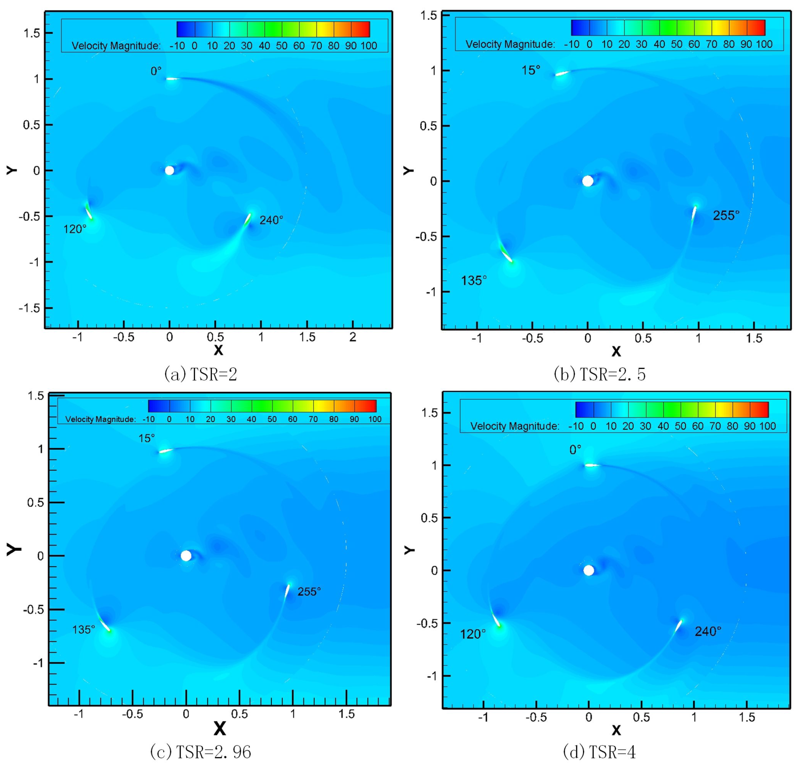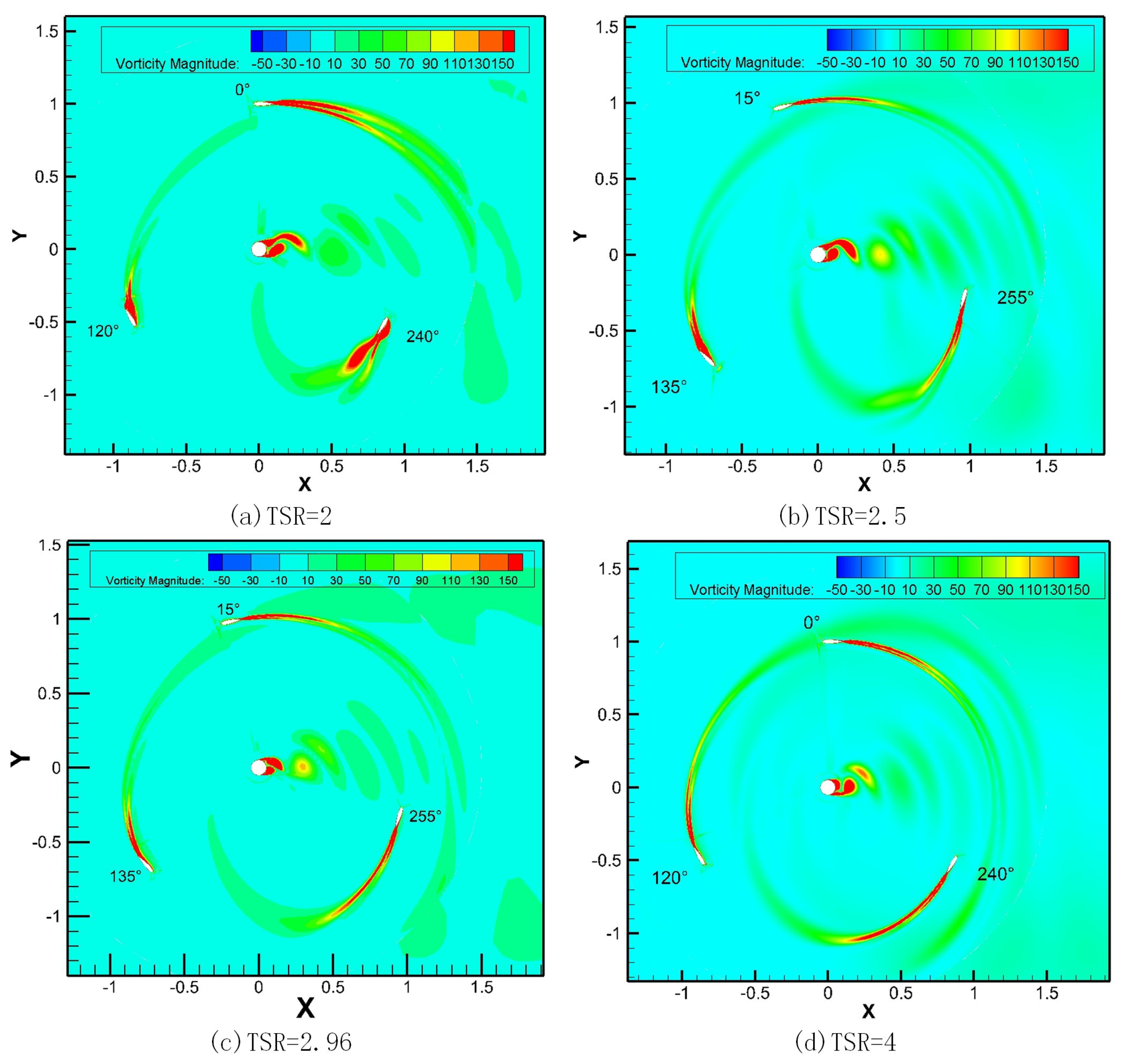Figure 30 shows the surrounding velocity flow field of J-shaped blade at azimuth angles of 60°, 90° and 120° before and after optimization. When the azimuth angle is at 60°, the velocity flow field and wake effect in the leading edge and middle of the blade are weakened after optimization. When the azimuth angle is at 90°, the velocity flow field at the leading edge of the optimized J-shaped blade increases, while the drag on the lower surface decreases and the wake flow weakens. When the azimuth angle is at 120°, the vortex on the lower surface of the blade is shedding, and the shedding vortex intensity of J-shaped blade decreases after correction. At the same time, because the radian of the lower surface of J-shaped blade decreases after correction, the blade torque increases when the azimuth angle is between 90° and 180°.

Figure 31 and Figure 32 shows the torque variation curve with azimuth at TSR = 1.5 and TSR = 2.96 before and after optimization of J-blade wind generator. As can be seen from Figure 31, when TSR = 1.5, the optimized J-blade’s instantaneous torque is significantly improved when the azimuth angle is between 60° and 120°, while when the azimuth angle is between 180° and 360°, the influence of vortex falling off on the optimized J-blade’s torque is greater, and the instantaneous torque is not as good as before. As can be seen from Figure 32, when TSR = 2.96, the optimized blade has little change in instantaneous torque when the azimuth angle is between 0° and 180°, and when the azimuth angle is between 180° and 360°, the instantaneous torque provided by the J-shaped blade is small or even negative, while the optimized J-shaped blade’s torque decreases when the azimuth angle is between 180° and 360°.

The maximum instantaneous torque change of blade after optimization is shown in

Table 5. Variation of maximum instantaneous torque of blades after optimization.

TSR	The Maximum Torque Increase (N·m)	Percentage Increase
0.5	8.82 N·m	43.23%
1	13.95 N·m	40.77%
1.5	16.80 N·m	35.68%
2	13.95 N·m	24.64%
2.5	8.54 N·m	14.06%
2.96	2.80 N·m	4.50%

. First of all, it can be seen that after optimization, the maximum blade torque increases when $\mathrm{TSR}\in [0.5,2.96]$, and the smaller the blade tip speed ratio is, the greater the increase range is, and the maximum torque at startup stage is significantly improved. When $\mathrm{TSR}=1.5$, the maximum increase of blade instantaneous maximum torque is $16.80 \mathrm{N}·\mathrm{m}$, when $\mathrm{TSR}=0.5$, the maximum increase of blade instantaneous maximum torque is 43.23%, and when $\mathrm{TSR}=2.96$, the maximum increase of blade maximum torque is 4.5%.

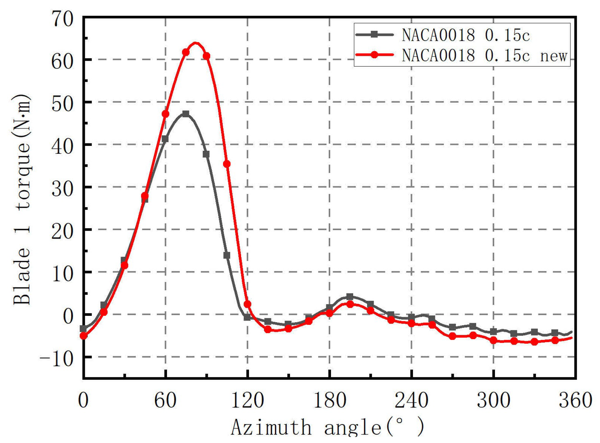
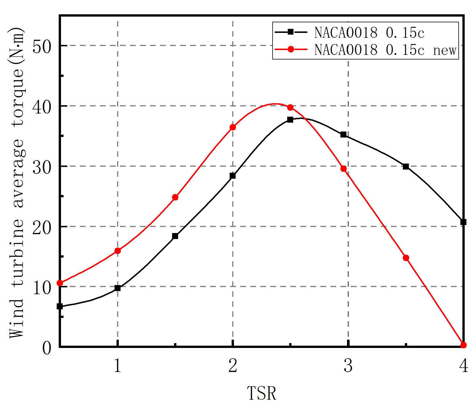
Figure 33 and Figure 34 show variation curves of instantaneous torque and average torque of J-blade wind generator before and after optimization. Figure 33 shows the wind generator’s instantaneous torque at $\mathrm{TSR}=1.5$. Since the torque of the wind generator is superposed by three blades with a difference of 120°, the optimized J-blade wind generator’s instantaneous torque increases greatly when the azimuth angles are selected in the intervals of [60°,120°], [180°,240°], or [300°,360°], corresponding to the azimuth angles of the blade’s instantaneous torque increase. It can be seen from Figure 34 that the average torque of the optimized wind generator increases when $\mathrm{TSR}\in [0.5,2.5]$, but decreases rapidly as the blade tip speed ratio continues to increase.

After optimization, the average torque change of offshore wind turbine is shown in

Table 6. Average torque variation of offshore wind turbine after optimization.

TSR	The Average Torque of the Fan Changes after Optimization	Percentage Increase
0.5	3.89 N·m	57.90%
1	6.23 N·m	64.05%
1.5	6.48 N·m	35.30%
2	8.10 N·m	28.55%
2.5	2.03 N·m	5.39%
2.96	−5.64 N·m	−16.02%

. It can be seen that after optimization, the average torque of the wind generator increases first and then decreases when $\mathrm{TSR}\in [0.5,2.96]$. When $\mathrm{TSR}=2$, the average torque of the offshore wind turbine is increased by 16.80 N·m at most, and when $\mathrm{TSR}=1$, the average torque of the offshore wind turbine is increased by 64.05% at most, but the average torque of the offshore wind turbine blade is reduced by 16.02% at $\mathrm{TSR}=2.96$. After optimization, the average torque of the wind generator is improved when $\mathrm{TSR}\in [0.5,2.5]$, and the improvement is more obvious when the blade tip ratio is low.

The change curve of wind energy capture rate of the J-blade wind generator with tip speed ratio before and after optimization is shown in Figure 35. It can be seen that the wind energy capture rate increases when $\mathrm{TSR}\in [0.5,2.96]$ after optimization, and the trend of 2D simulation and 3D simulation is consistent. Due to the influence of space turbulence, the wind energy capture rate of 3D simulation is slightly lower than that of the 2D simulation, and the optimized wind energy capture rate decreases when $\mathrm{TSR}\in [2.96,4]$.

The wind energy capture rate of the two-dimensional wind generator before and after optimization when $\mathrm{TSR}\in [0.5,2.96]$ is shown in

Table 7. Changes of wind energy capture rate of two-dimensional offshore wind turbines before and after optimization.

TSR	Before Optimization	The Optimized
0.5	1.36%	1.90%
1	3.93%	3.45%
1.5	11.14%	7.78%
2	22.97%	10.78%
2.5	38.16%	7.80%
2.96	42.18%	−1.07%

. When $\mathrm{TSR}=2$, the maximum increase of wind energy capture rate is 10.78%, and the maximum of wind energy capture rate is 45.96% when $\mathrm{TSR}=2.5$ after optimization. It can be seen that after blade optimization, the wind energy capture rate at low blade tip speed ratio is significantly improved.

6. Conclusions

The main content of this study is to improve the performance of the Darrieus vertical axis offshore wind turbine, including wind capture efficiency and torque variation. The simulation results based on iteration design of compactness of offshore wind turbine have a good fit with the experimental results. The two-dimensional simulation ignores the influence of spatial turbulence and the connecting arm of the wind generator, and the result of the high blade tip speed ratio is larger, and the optimal wind energy capture rate is about 3.5. The 3D simulation results are closer to the experimental results, and the optimal wind energy capture rate is about $\mathrm{TSR}=2.96$. First, the influence of the change of the upper surface of J-blade on the performance of the offshore wind turbine is studied. The results show that the change of the upper surface of J-blade has little influence on the performance of the offshore wind turbine at low wind speed and low blade tip ratio. At high wind speed and high blade tip ratio, the farther the distance from the upper surface of J-blade to the leading edge, the less the performance decreases. Second, the performance changes of offshore wind turbines before and after the optimization of the lower surface of J-shaped blades are studied. The results show that the wind energy capture rate of offshore wind turbines after the optimization of the lower surface increases by 10.78% at $\mathrm{TSR}=2$ compared with that before the optimization, while the performance decreases rapidly when the blade tip ratio is high.

References

1. Liu, J.; Lin, H.; Zhang, J. Review on the technical perspectives and commercial viability of vertical axis wind turbines. Ocean Eng. 2019, 182, 608–626. [Google Scholar] [CrossRef]
2. Senad, A.; Sandra, E.; Hans, B. A Review of Research on Large Scale Modern Vertical Axis Wind Turbines at Uppsala University. Energies 2016, 9, 570. [Google Scholar]
3. Hara, Y.; Jodai, Y.; Okinaga, T.; Furukawa, M. Numerical Analysis of the Dynamic Interaction between Two Closely Spaced Vertical-Axis Wind Turbines. Energies 2021, 14, 2286. [Google Scholar] [CrossRef]
4. Shiraz, M.Z.; Dilimulati, A.; Paraschivoiu, M. Wind power potential assessment of roof mounted wind turbines in cities. Sustain. Cities Soc. 2019, 53, 101905. [Google Scholar] [CrossRef]
5. Fanel Dorel, S.; Adrian Mihai, G.; Nicusor, D. Review of Specific Performance Parameters of Vertical Wind Turbine Rotors Based on the SAVONIUS Type. Energies 2021, 14, 1962. [Google Scholar] [CrossRef]
6. Liu, K.; Yu, M.; Zhu, W. Enhancing wind energy harvesting performance of vertical axis wind turbines with a new hybrid design: A fluid-structure interaction study. Renew. Energy 2019, 140, 912–927. [Google Scholar] [CrossRef]
7. Lei, H.; Zhou, D.; Lu, J.; Chen, C.; Han, Z.; Bao, Y. The impact of pitch motion of a platform on the aerodynamic performance of a floating vertical axis wind turbine. Energy 2017, 119, 369–383. [Google Scholar] [CrossRef]
8. Bianchini, A.; Ferrara, G.; Ferrari, L.; Magnani, S. An Improved Model for the Performance Estimation of an H-Darrieus Wind Turbine in Skewed Flow. Wind Eng. 2012, 36, 667–686. [Google Scholar] [CrossRef]
9. Guo, J.; Lei, L. Flow Characteristics of a Straight-Bladed Vertical Axis Wind Turbine with Inclined Pitch Axes. Energies 2020, 13, 6281. [Google Scholar] [CrossRef]
10. Hand, B.; Kelly, G.; Cashman, A. Numerical simulation of a vertical axis wind turbine airfoil experiencing dynamic stall at high Reynolds numbers. Comput. Fluids 2017, 149, 12–30. [Google Scholar] [CrossRef]
11. Tjiu, W.; Marnoto, T.; Mat, S.; Ruslan, M.H.; Sopian, K. Darrieus vertical axis wind turbine for power generation I: Assessment of Darrieus VAWT configurations. Renew. Energy 2015, 75, 50–67. [Google Scholar] [CrossRef]
12. Li, L.; Chopra, I.; Zhu, W.; Yu, M. Performance Analysis and Optimization of a Vertical-Axis Wind Turbine with a High Tip-Speed Ratio. Energies 2021, 14, 996. [Google Scholar] [CrossRef]
13. Mellstig, E.G. SeaTwirl in Dagens Industri. 2020. Available online: https://seatwirl.com/news/seatwirl-in-dagens-industri/ (accessed on 13 October 2020).
14. Zhang, T.; Elsakka, M.; Huang, W.; Wang, Z.; Ingham, D.B.; Ma, L.; Pourkashanian, M. Winglet design for vertical axis wind turbines based on a design of experiment and CFD approach. Energy Convers. Manag. 2019, 195, 712–726. [Google Scholar] [CrossRef]
15. Mohamed, O.S.; Ibrahim, A.A.; Etman, A.K.; Abdelkader, A.; Elbaz, A. Numerical investigation of Darrieus wind turbine with slotted airfoil blades. Energy Convers. Manag. X 2020, 5, 100026. [Google Scholar] [CrossRef]
16. Zamani, M.; Maghrebi, M.J.; Varedi, S.R. Starting torque improvement using J-shaped straight-bladed Darrieus vertical axis wind turbine by means of numerical simulation. Renew. Energy 2016, 95, 109–126. [Google Scholar] [CrossRef]
17. Zamani, M.; Nazari, S.; Moshizi, S.A.; Maghrebi, M.J. Three dimensional simulation of J-shaped Darrieus vertical axis wind turbine. Energy 2016, 116, 1243–1255. [Google Scholar] [CrossRef]
18. Mohamed, M. Criticism study of J-Shaped darrieus wind turbine: Performance evaluation and noise generation assessment. Energy 2019, 177, 367–385. [Google Scholar] [CrossRef]
19. Brusca, S.; Lanzafame, R.; Messina, M. Design of a vertical-axis wind turbine: How the aspect ratio affects the turbine’s performance. Int. J. Energy Environ. Eng. 2014, 5, 1–8. [Google Scholar] [CrossRef] [Green Version]
20. Paraschivoiu, I. Double-multiple streamtube model for studying vertical-axis wind turbines. J. Propuls. Power 1988, 4, 370–377. [Google Scholar] [CrossRef]
21. Li, Q.; Maeda, T.; Kamada, Y.; Murata, J.; Furukawa, K.; Yamamoto, M. The influence of flow field and aerodynamic forces on a straight-bladed vertical axis wind turbine. Energy 2016, 111, 260–271. [Google Scholar] [CrossRef]
22. Lee, Y.T.; Lim, H.C. Numerical study of the aerodynamic performance of a 500W Darrieus-type vertical-axis wind turbine. Renew. Energy 2015, 83, 407–415. [Google Scholar] [CrossRef]
23. Lam, H.; Peng, H. Study of wake characteristics of a vertical axis wind turbine by two- and three-dimensional computational fluid dynamics simulations. Renew. Energy 2016, 90, 386–398. [Google Scholar] [CrossRef]
24. Sajid, M. Effect of vortices on power output of vertical axis wind turbine (VAWT). Sustain. Energy Technol. Assess. 2020, 37, 100586. [Google Scholar]
Figure 1. Offshore floating vertical axis offshore wind turbine [13].
Energies 14 06426 g001
Figure 2. Curve of wind energy capture rate changing with blade tip speed ratio [19]. (a) the Reynolds number (5 ∗ 106) of the NACA0018 airfoil wind generator, (b) the Reynolds number (1 ∗ 106) of the NACA0018 airfoil wind generator, (c) the Reynolds number (3.6 ∗ 105) of the NACA0018 airfoil wind generator, (d) the Reynolds number (1.6 ∗ 105) of the NACA0018 airfoil wind generator.
Energies 14 06426 g002
Figure 3. Iterative design process of offshore wind turbine.
Energies 14 06426 g003
Figure 4. Model of symmetrical airfoil J-blade offshore wind turbine.
Energies 14 06426 g004
Figure 5. J-blade vertical axis offshore wind turbine.
Energies 14 06426 g005
Figure 6. The influence of structural changes of J-shaped blades on offshore wind turbine performance. (a) the structural of J-shaped blades, (b) the structural (0.05c = 6.8 mm) of J-shaped blades, (c) the structural (0.01c = 13.6 mm) of J-shaped blades, (d) the structural (0.15c = 20.4 mm) of J-shaped blades, (e) the structural (0.25c = 34 mm) of J-shaped blades, (f) the structural (0.15c = 20.4 mm) of J-shaped blades.
Energies 14 06426 g006
Figure 7. Two-dimensional computational domain model.
Energies 14 06426 g007
Figure 8. Three-dimensional computational domain model.
Energies 14 06426 g008
Figure 9. Three-dimensional computational mesh.
Energies 14 06426 g009
Figure 10. Curve of wind energy capture rate changing with the number of grids.
Energies 14 06426 g010
Figure 11. y + distribution near offshore wind turbine blade and spindle ( TSR = 2.96 ).
Energies 14 06426 g011
Figure 12. J-blade wind generator 2D and 3D mesh.
Energies 14 06426 g012
Figure 13. y + distribution around J-shaped blade and spindle ( TSR = 2.96 ).
Energies 14 06426 g013
Figure 14. Curve of offshore wind turbine torque changing with azimuth ( TSR = 2.96 ).
Energies 14 06426 g014
Figure 15. Torque curves of offshore wind turbine under different turbulence models.
Energies 14 06426 g015
Figure 16. Velocity cloud diagram of two-dimensional wind generator with different TSR.
Energies 14 06426 g016
Figure 17. Vorticity diagram of three-dimensional offshore wind turbine with different TSR ( V o r t i c i t y M a g n i t u d e = 50 s 1 ).
Energies 14 06426 g017
Figure 18. Vorticity diagram of two-dimensional wind generator with different TSR.
Energies 14 06426 g018
Figure 19. Curve of torque changing with azimuth.
Energies 14 06426 g019
Figure 20. Curve of maximum torque changing with blade tip speed ratio.
Energies 14 06426 g020
Figure 21. Curve of torque changing with azimuth.
Energies 14 06426 g021
Figure 22. Average torque curve with blade tip speed ratio.
Energies 14 06426 g022
Figure 23. Wind energy capture rate curve.
Energies 14 06426 g023
Figure 24. J-shaped blade velocity flow field.
Energies 14 06426 g024
Figure 25. TSR = 1.5 instantaneous torque curve of J-shaped blade.
Energies 14 06426 g025
Figure 26. TSR = 2.96 instantaneous torque curve of J-shaped blade.
Energies 14 06426 g026
Figure 27. Curve of offshore wind turbine torque changing with azimuth ( TSR = 1.5 ).
Energies 14 06426 g027
Figure 28. Curve of blade average torque changing with blade tip speed ratio.
Energies 14 06426 g028
Figure 29. Wind energy capture rate of wind generator with two-dimensional J-blade.
Energies 14 06426 g029
Figure 30. Velocity flow field around J-shaped blade before and after optimization.
Energies 14 06426 g030
Figure 31. Torque of J-blade wind generator before and after optimization ( TSR = 1.5 ).
Energies 14 06426 g031
Figure 32. Torque of J-blade wind generator before and after optimization ( TSR = 2.96 ).
Energies 14 06426 g032
Figure 33. Variation curve of instantaneous torque with azimuth before and after optimization.
Energies 14 06426 g033
Figure 34. Variation curve of average torque with tip speed ratio before and after optimization.
Energies 14 06426 g034
Figure 35. Wind energy capture rate of J-blade wind generator before and after optimization.
Energies 14 06426 g035