Global Sensitivity Analysis Applied to Train Traffic Rescheduling: A Comparative Study

Abstract

The adjustment of rail traffic in the event of an electrical infrastructure disruption presents an important decision-making process for the smooth operation of the network. Railway systems are complex, and their analysis relies on expensive simulations, which makes incident management difficult. This paper proposes the use of sensitivity analysis in order to evaluate the influence of different traffic adjustment actions (e.g., spacing between trains and speed reduction) on the train supply voltage, which must never drop below the critical value prescribed by technical standards. Three global sensitivity analysis methods dedicated to black box, multivariate, nonlinear models are considered: generalized Sobol indices, energy distance-based indices, and regional sensitivity analysis. The three methods are applied to a simple traffic rescheduling test case and give similar results, but at different costs. Regional sensitivity analysis appears to be the most suitable method for the present application: it is easy to implement, rather fast, and accounts for constraints on the system output (a key feature for electrical incident management). The application of this method to a test case representative of a real rescheduling problem shows that it provides the information needed by the traffic manager to reschedule traffic in an efficient way. The same type of approach can be used for any power system optimization problem with the same characteristics.

1. Introduction

The increasing demand for rail transport leads to a densification of the traffic and a growing impact of any unexpected event, such as track damage, rolling stock breakdown, or signal failure. Due to the cascade effect, a single train delay may affect a large number of trains. In such a case, the timetable deviation is small and the perturbation is therefore referred to as a disturbance. On the other hand, a technical incident causing the partial or total blocage of a track results in large perturbation which is known as disruption. Disruptions require not only the timetable, but also the duties for rolling stock and crew to be modified.

Rescheduling the traffic is an important task for limiting the inconvenience for passengers (e.g., delays, broken connections, and crowded trains) and the operator (additional costs). Currently, this task is performed manually, but a lot of research is being conducted to develop numerical optimization methods and provide intelligent decision support. A key problem is the development of fast methods for real-time operations. Contingency plans may also be built in advance, but they cannot be optimal for all situations. In [1], the authors provide a good introduction to the subject.

The present paper deals with disruption due to the failure of electrical equipment that limits the power available for the trains, and consequently affects the traffic in the area. While the literature on disturbance management is abundant (see for example [2,3,4,5]), less work has been published on disruption management. Most studies deal with the impact of the unavailability of one or several tracks during a certain time. In [6], the partial or complete blockage of a track is managed using three types of rescheduling action: delaying, cancelling, and reversing trains at the blockage. An integer programming formulation is proposed. The test case is a part of the Netherlands network and it is shown that delaying some trains can significantly reduce the number of cancelled trains. In [7], the outcome of short-turning management in the case of a complete blockage is considered. The paper considers short-turning time and short-turning before the blockage is introduced. Mixed integer linear programming is used to minimize a cost function with cancellation and arrival delay penalties. In [8], a mixed-integer linear programming model is also used, but in the case of the complete blockage of a high-speed line in China. Trains do not turn back and wait in a station. The issue is deciding in which station each train must wait, in which order trains must go when the blockage is over, and which trains should be cancelled. In [9], the authors consider the temporary blockage of a two-way track and choose to reschedule only the trains that conflict due to the blockage. Train cancellation is not considered and the test case remains rather simple. In [10], three objectives are considered: passenger satisfaction, the operational costs, and the deviation from the initial schedule. MILP optimization is performed with respect to the first objective, under the constraint of maximum values for the two others. A three-dimensional Pareto frontier is then built, and this demonstrates that a reasonable tradeoff between the three objectives can be reached. These examples of work do not constitute an exhaustive review and we refer the reader to [11,12] for in-depth surveys on train timetabling problems.

All these studies are based on simplified models of the railway network, namely graphs, whose branches are the tracks between stations or bifurcations and are characterized by given train flux capacities (e.g., train/hour). Such models are well suited for the construction of schedules for given track capacities, but detailed models that account for all physical and technical constraints of the system must be used afterwards to check the feasibility of the proposed solution.

The present work addresses the specific case of the loss of electrical equipment, such as a feeding substation. This loss can be due to either a technical failure or a planned maintenance operation. It decreases the electric power available for the train traction, and consequently requires the traffic to be reduced. This is a disruption problem that can be managed with rescheduling actions, such as increasing the time interval between trains or locally reducing their speed. The key problem is optimally rescheduling the traffic within the physical limits imposed by the power supply system. Unlike the previously mentioned research papers, this problem requires a detailed electro-mechanical model of the system, able to calculate the instantaneous power required by each train and account for the physical, nonlinear behavior of the power network. Such models are computationaly intensive and the optimization methods used for usual scheduling problems do not apply. To the best of our knowledge, this type of disruption problem is not addressed in the scientific literature.

Direct optimization would involve solving a computationally intensive, nonlinear, non-differentiable, multi-objective problem, with constraints on the model outputs. As this is a too difficult problem, the first contribution of this paper is to propose a methodology based on global sensitivity analysis to rank the rescheduling variables according to their influence on the output voltage, choose the most important ones, and simplify the optimization problem.

Choosing the right sensitivity analysis method is a problem in itself, because we are dealing with a nonlinear, black box model, whose outputs are time series that are subjected to inequality constraints. Our second contribution is an extensive literature search and the identification of three global sensitivity analysis methods suitable for this type of problem: generalized Sobol indices, energy distance-based indices, and regional sensitivity analysis. A comparative analysis of these methods is presented, and their performances are assessed in the case of a simplified rescheduling test problem. The third contribution is to apply the proposed methodology to a test case that is representative of a real rescheduling study. The results provide the decision maker with objective indicators for choosing the most efficient rescheduling actions. Beyond the specific problem of train traffic rescheduling, the proposed methodology can be applied to power engineering problems with similar characteristics, while the comparative analysis provides guidelines for choosing a suitable sensitivity analysis method.

The remainder of the paper is organized as follows. Section 2 describes the railway system, as well as the rescheduling problem and how it is formalized as an adjustment model. Section 3 presents a sensitivity analysis review and identifies three sensitivity analysis methods suitable for multivariate outputs. In Section 4, the three methods are applied to a simple traffic rescheduling test case and their performances are compared. Section 5 considers a complex test case and shows that our methodology provides useful information for the management of real incidents. Section 6 summarizes the work and its conclusions.

2. Problem Statement

2.1. System Description

Railway electrical networks (either AC or DC ) are complex system that provide the power needed by the trains. The main elements are the power substations, the overhead lines (catenary), the trains, and the rails (return conductor). Paralleling stations allow the line resistance to be adjusted according to the position of the trains. In an AC network, switching elements separate the portions of lines supplied by different substations.

Railway electrical networks are complex systems with many components. The trains are moving loads and the network topology changes according to their positions. Furthermore, the trains themselves become power sources during the process of regenerative braking. The analysis of railway networks requires detailed models and relies on numerical simulation.

2.2. Simulator Description

Railway simulators calculate all the physical quantities needed by the engineer for given infrastructures and scheduled traffic: voltages, currents, train position and speed, and heatings. In the present work, we use ESMERALDA NG, a simulator developed and distributed by SNCF Réseau [13].

ESMERALDA NG relies on models that result from the SNCF’s expertise and are detailed enough to allow precise determination of all the quantities aforementioned, with a strong coupling between mechanical and electrical equations. The input data are the physical characteristics of the railway infrastructure (tracks and electrical equipment), the rolling stock (locomotives, cars, and engines), and the scheduled traffic (type of trains, departure and arrival times at various points, and speed profiles). Given this data, the equations of the electrical circuit are coupled with the equations of the train dynamics, and are solved step by step in order to determine the voltage at all nodes of the circuit and the position of the different trains at all time steps (Figure 1). All other quantities of interest (catenary current, substations power, transformer heating, etc.) are post-processed.

ESMERALDA NG is used by SNCF Réseau and other service companies for electricity infrastructure-sizing studies involving all types of traffic: urban (RER), regional, high speed (TGV), and freight. Depending on the size of the studied network, the simulation time varies from a few minutes to an hour, with a typical duration of around ten minutes for the simulation of two hours of traffic at a regional scale.

An important feature of ESMERALDA NG is that it accounts for the engine regulation mechanisms that prevent an excessive voltage drop along the catenary. At each step of time, if the catenary voltage of a train drops below a critical value, the power supplied to this train is limited in order to keep the catenary voltage within a range defined according to specific standards. Consequently, the speed of a train in this position would be smaller than expected. This situation means that the electrical network is overloaded and that one should either reinforce the electrical infrastructure (in a design and sizing study) or reschedule the traffic within the limits of the feeding network capacity (in an incident management study).

2.3. Managing the Unavailability of an Electrical Equipement

Technical problems or maintenance operations can cause the loss of electrical equipment—a feeding substation, for example—and reduce the power that the feeding network can deliver to the trains in the area affected by the incident. If the power still available in this degraded mode is too low for the scheduled traffic, the traffic must be adjusted to ensure that the electrical network always operates under good conditions, or, more specifically, that the catenary voltage never drops below the critical value defined by particular standards.

Operators in charge of handling such incidents adjust the traffic schedule as best as possible and try to limit the loss of transportation capacity of the affected lines. Based on their expertise, they define adjustment actions, such as increasing the time interval between consecutive trains, or reducing the speed limit in the area affected by the incident. These actions modify the spatiotemporal profile of the network load, and the goal is to determine various possible combinations of actions such that the catenary voltage remains within the prescribed limits. Following a trial-and-error approach, operators run simulations in order to determine acceptable sets of adjustement actions and choose the most performant one. Several performance criteria can be considered: train density (i.e., the number of trains that can circulate during a given time interval), global electric consumption, substation transformer heating, etc.

The present trial-and-error approach relies on operator know-how and is not efficient, especially because it requires computationally intensive simulations. Given the financial cost of incidents on electrical infrastructure, SNCF Réseau, the company responsible for the management and maintenance of railway infrastructure in France, has launched a project whose goal is to develop numerical tools for improving the rescheduling process. The proposed approach and the results are presented in this paper.

2.4. Mathematical Formalization of the Traffic Adjustment Problem

Rescheduling traffic consists of modifying the scheduled traffic so as to to adjust the spatiotemporal load of the feeding network and keep the catenary voltage within acceptable limits at all points and at all times.

In practice, rescheduling operators do not act train-by-train, but define global adjustment actions that preserve the regularity of schedules and train speed profiles. Each action is modeled by a macroscopic adjustment variable, denoted as $X_i$ hereafter. For example, the action of spacing out train departures is modeled by a variable that quantifies the increase in the time interval between two successive departures of a series of trains. The action of slowing down trains between two given points on the line is modeled by a variable that quantifies the reduction of the limiting speed. A set of actions is represented by the vector $X=\left(X_1, \dots , X_p\right)$ and interval constraints ${\left(X_{i min}\le X_i\le X_{i max}\right)}_{i=1,p}$, where $p$ is the number of adjustment variables.

The adjustment model is a layer that encompasses the simulator (Figure 2). A pre-processing step consists of modifying the initial traffic data in accordance with the actions defined by the adjustment variables. Then, the simulation itself is run and the outputs of the adjustment model are directly the outputs of the simulator, of the shape $Y=\left(Y\left(t_1\right),Y\left(t_2\right),\dots ,Y\left(t_m\right)\right)$, where $m$ is the number of time steps. The catenary voltages shown on Section 4 are examples of such dynamic outputs, with one voltage series per train. The simulator outputs are supplemented by post-processed performance criteria.

2.5. Inadequacy of Classical Optimization Methods and Proposed Methodology

The adjustment model is complex, in the sense that it is based on a nonlinear railway simulator with a large number of variables, dynamic outputs, and a high computational cost (typically around ten minutes for the simulation of two hours of traffic on a regional network). For example, suppose a traffic of 200 trains, fed by a network with 10 substations. The number of simulator input variables is greater than 1000. The number of dynamic outputs (time series) is also important: at least one for each train. One hour of simulated traffic corresponds to approximately 5000 time steps, and the operational constraints need to be checked at each time step (catenary voltage, cable and transformer heating, etc.).

Given the characteristics of the traffic adjustment problem, direct optimization cannot be envisaged, and so we have chosen to use sensitivity analysis in order to quantify the influence of the different adjustment variables on the catenary voltage and identify the most important adjustment actions that allow an efficient rescheduling. This allows us to reduce the number of adjustment variables and to solve a simplified optimization problem.

The next section presents an overview of sensitivity analysis methods, before focusing on three global sensitivity analysis methods that are suitable for black box models with dynamic outputs. Each method uses a specific characteristic of the output to build global sensitivity indices.

3. Global Sensitivity Analysis for Multivariate Outputs

3.1. Overview of Sensitivity Analysis

Sensitivity analysis aims at studying the behavior of a model by assessing how the input variations impact the output variations, both in a qualitative and quantitative way. The reader can find a general introduction to sensitivity analysis in [14] and complete reviews in [15,16,17]. The present section gives a quick overview of the different existing methods.

The first historical approach is known as local sensitivity analysis. This deterministic approach quantifies the impact of small input perturbations by estimating the partial derivatives of the model [18]. This approach is valid only around the analyzed point. It does not perform any exploration of the variation space of the inputs. To overcome this limitation, global approaches were constructed within a statistical framework that can account for the whole range of input variation.

Among global methods, screening techniques are based on a discretization of the inputs in levels. Dedicated to models with a large number of inputs (several tens), they perform a fast exploration of the model behavior over the entire input space in order to identify the non-influential inputs and simplify the model by fixing these inputs to nominal values. The most widely used screening approach is the “one at a time” method, where input variables are modified in turn [19]. Screening methods provide qualitative information that can be used to diminish the number of inputs and simplify the model, but the results should be carefully interpreted when dealing with nonlinear models [20]. A more general approach is to use quantitative methods based on statistics. There are indices based on linear regression, and others on linear or quadratic ANOVA (analysis of variance). In the case of nonlinear models, Sobol indices [21,22,23], based on the concept of functional decomposition of variance, are widely used [24].

Sobol indices provide sensitivity indices which account for the whole range of the input variation globally. Other methods have been proposed in order to identify the parts of the input range which contribute the most to the output variation. The so-called “contribution to the sample mean” plot (CSM) [25] and “contribution to the sample variance” plot (CSV) [1,26] are graphical tools which allow researchers to localize specific regions of the input space that contribute greatly to the output variation. This information can be used to reduce the output variance by adjusting the range of input variation. Other examples of works where the authors analyze the output variance in order to measure the influence of different regions of the input space are [27,28].

Sensitivity analysis was first developed for scalar output variables, but the outputs of computational models are often time (or space) series. In such cases, time-dependent sensitivity indices can be defined, but these fail to give any synthetic information about the whole output time series, despite the strong redundancy of the information. In [29], the authors propose performing a sensitivity analysis on the expansion of the output on a well-chosen functional basis. An approach based on polynomial chaos expansion is proposed in [30]. In [31,32], a problem-independent approach based on covariance decomposition is proposed in order to define global indices accounting for the whole temporal domain, and this approach is compared to a principal component analysis. This concept of generalized Sobol indices is further mathematically developed in [33,34].

Sobol's indices are based on the comparison of variances. Except for Gaussian distributions, this information is not sufficient to characterize the distributions of the output, which leads to a loss of information [18]. To overcome this limitation, ”moment-independent methods”, accounting for the entire output distribution, have emerged. These methods are based on the concept of distance between distributions. The cumulative distributions or the probability densities are used in [35,36,37], but this approach is limited to scalar outputs. An interesting approach based on “energy distance” which is suitable for series outputs has been introduced in [38].

Another issue with sensitivity analysis is identifying which part of the input space is responsible for leading the model output in a given region of the output space. This issue typically arises when the model output must meet some constraint, such as being above or below a given threshold. In terms of sensitivity analysis, it is necessary to determine whether a given input has an influence on wheather this output constraint is met. Regional sensitivity analysis, based on Monte Carlo filtering, was proposed to adress this issue [39,40,41].

In the case of the traffic adjustment problem, we are dealing with outputs that are time series which are subjected to particular constraints. Hence, we have successively tested generalized Sobol indices (Section 3.3), energy distance-based indices (Section 3.4), and regional sensitivity analysis (Section 3.5).

Sensitivity analysis methods differ from each other in the way they define the sensitivity measurement, but they all rely on the following three phases: (i) sampling of the input variation space, (ii) computation of the model for each sample of the input space, and (iii) computation of sensitivity indices according to the considered principle. The sampling phase is crucial for an efficient estimate of the sensitivity indices. A short review of the main techniques is given in the Section 3.2.

3.2. Sampling Phase

Global sensitivity analysis methods are based on statistics and the Monte Carlo simulation. A sample of $N$ points is randomly generated in the input space, forming a matrix of $N$ rows and $p$ columns, where $p$ is the number of inputs. The model is applied to each of the points and each dynamic output forms a matrix of $N$ rows and $m$ columns, where $m$ is the dimension of the considered output. Figure 3 defines the notations that will be used in the rest of the text, for a single output $Y$ (for example, the catenary voltage series of one particular train). The reader should keep in mind that there are many such outputs.

To be meaningful, sensitivity analysis must rely on a good sampling, with enough points that are well distributed across the whole input space. Different techniques exist for sampling independent variables. The challenge is to obtain a good compromise between accurate sensitivity indices and reasonable computation time.

The historical Monte Carlo method relies on the basic random sampling of each input. In practice, this results in a non-uniform coverage of the space, with clusters and gaps. Stratified sampling [42] mitigates the problem by partitioning the space into subsets from which samples are selected with given probabilities. The difficulty lies in the choice of the space partitioning and the associated probabilities. Latin hypercube sampling [43] was designed as a combination of the random and stratified techniques and was designed to generate a better sampling of the input than random sampling with an easier implementation than the stratified method. Details of the methods and a comparison of their performances can be found in [43,44], for example. Another widespread method is quasi-random sampling, also known as low discrepancy sampling, based on the Sobol sequences [45]. This last method provides a good distribution of the samples by taking into account the points previously sampled, thus avoiding the appearance of clusters and gaps. Comparisons show that quasi-random sampling allows faster statistic convergence than Latin hypercube sampling [46,47]. For this reason, quasi-random sampling has been used in the present work. Details on the method implementation can be found in [48,49]. Different implementations can be found in C, C++, Python, Fortran 90 [50], and Julia [51].

3.3. Generalized Sobol Indices

3.3.1. Sobol Indices for Scalar Outputs

Sobol indices were developped for nonlinear black box models with a limited number of independent input variables. They facilitate the ordering of inputs according to their influence on the output. They can also characterize interactions between the inputs.

Sobol indices were first proposed in 1993 [21] and improved during the following decade [22,23,52,53]. They are based on the Hoeffding decomposition [54] of the model being studied, and the decomposition of the output variance into a combination of conditional variances based on the independent inputs (ANOVA representation). First and second order Sobol indices, denoted respectively by $S_i$ and $S_{ij}$, are defined by:

$$S_i=\frac{Var\left[E\left(Y|X_i\right)\right]}{Var\left(Y\right)}$$

and

$$S_{ij}=\frac{Var\left[E\left(Y|X_i,X_j\right)\right]-Var\left[E\left(Y|X_i\right)\right]-Var\left[E\left(Y|X_j\right)\right]}{Var\left(Y\right)}$$

Higher order indices can also be defined. The values of the coefficients are between 0 and 1, and the sum of all coefficients is 1. Generally, for computational cost reasons, only the first order indices are estimated.

Interestingly, first order Sobol indices can be introduced in the following intuitive way [53]. The influence of the input variable $X_i$ on the output $Y$ can be assessed by observing $V\left(Y|Xi=x_i^{\ast }\right)$, the conditional variance of $Y$, $X_i$ being fixed to a given value $x_i^{\ast }$. As $x_i^{\ast }$ may take any value in its variation range, its global influence is given by $E\left[V\left(Y|X_i\right)\right]$, the expectation of the conditional variance for all possible values of $x_i^{\ast }$. The more important the contribution of $X_i$ to the variance of $Y$, the smaller the value of $E\left[V\left(Y|X_i\right)\right]$. The total variance can be written as: $V\left(Y\right)=V\left(E\left[Y|X_i\right]\right)+E\left[V\left(Y|X_i\right)\right]$. Hence, the term $V\left(E\left[Y|X_i\right]\right)$ is also an indicator of the sensitivity of Y with respect to $X_i$. The more $X_i$ contributes to $V\left(Y\right)$, the higher $V\left(E\left[Y|X_i\right]\right)$ will be. The normalization of $V\left(E\left[Y|X_i\right]\right)$ allows the retrieval of $S_i$.

3.3.2. Generalized Sobol Indices

When the model output is a time series, generalized Sobol indices can be used to provide sensitivity information accounting for the whole temporal domain [33,34]. Generalized Sobol indices are based on the covariance matrix of $Y$, which characterizes the statistical interactions between the values of the output at different time steps. This matrix is defined by:

$$Cov\left(Y\right)={\left[Cov\left(Y\left(t_k\right),Y\left(t_l\right)\right)\right]}_{\begin{array}{c}1\le k\le m\\ 1\le l\le m\end{array}}$$

Using the Hoeffding decomposition of the model $Y=f\left(X_i\right)$ [54], the covariance matrix of $Y$ is partitioned into a sum of covariance matrices that characterize the influence of each input and their interactions. This matrix relation is projected into the space of real numbers by taking its trace, while generalized first order indices are defined by:

$$S_i\left(Y\right)=\frac{{{\displaystyle \sum }}_{k=1}^{m}Var[E(Y\left(t_k\right)|X_i)]}{{{\displaystyle \sum }}_{k=1}^{m}Var\left(Y\left(t_k\right)\right)}$$

The numerator is the sum of the first order effects of $X_i$ at the different time steps, and the denominator is the sum of the variances of the model output at the different time steps. Classical Sobol indices are retrieved for $m=1$.

3.3.3. First Order Sobol Indices Estimation

The papers [55,56] compare different numerical techniques that have been proposed to estimate the Sobol indices. In the present work, we use the most efficient one, proposed in [53]. The principle of the computation is as follows. The variances are calculated from the mathematical expectations according to the general relation:

$$Var\left(Y\right)=E\left(Y^2\right)-E{\left(Y\right)}^2$$

and the expectations are approximated by the mean estimator:

$$E\left(Y\right)\approx \frac{1}{N}{\displaystyle \sum }_{i=1}^N{y}_i$$

where the $y_i$ represents N realizations of the random variable Y.

We must estimate:

$$S_i=\frac{Var\left[E\left(Y|X_i\right)\right]}{Var\left(Y\right)}=\frac{E\left[E{\left(Y|X_i\right)}^2\right]-E{\left[E\left(Y|X_i\right)\right]}^2}{E\left(Y^2\right)-E{\left(Y\right)}^2}$$

Four mathematical expectations are to be estimated, two of which are conditional on the given $X_i.$ The terms of the denominator are straightforward, but the terms of the numerator require freezing the input variable $X_i$. For this, the algorithm uses (p + 1) sample matrices of identical sizes, according to the procedure described in Appendix A. The computation of the indices themselves is straightforward, but it requires N$\times$(p + 1) evaluations of the model. The algorithm also applies to generalized indices.

The sensitivity analysis method proposed by Sobol allows the calculation of all the sensitivity indices, including the interaction indices and the total effect indices relating to the input variables. As these sensitivity indices are based on the variance of the outputs, however, they may lack accuracy. To overcome this limitation, moment-independent methods have been proposed. The next section presents a method based on energy distance.

3.4. Sensitivity Analysis Based on Energy Distance between Distributions

3.4.1. Energy Distance

The energy distance is a statistical distance between two distributions of random vectors that can be used to test if these distributions are identically distributed [38]. This distance has the advantage of being moment independant.

Let us denote by X and Y two independent random vectors of size N. The energy distance between X and Y is define by:

$$ℰ\left(X,Y\right)=2\mathrm{E}\parallel X-Y\parallel -\mathrm{E}\parallel X-X^{\prime }\parallel -\mathrm{E}\parallel Y-Y^{\prime }\parallel$$

where E is the expectation, $\left||.|\right|$ is the Euclidian norm,$X^{\prime }$ and $Y^{\prime }$ are identically distributed copies of X and Y, and $\mathrm{E}\parallel X\parallel$ and $\mathrm{E}\left|\left|Y\right|\right|$ are finite.

A fundamental property of energy distance is that $ℰ\left(X,Y\right)=0 iif X and Y$ are identically distributed [57]. This function can be expressed by the characteristic function (the inverse Fourier transformation of the density) [58,59]. The energy distance is independent of the shape of the distribution, and therefore accurately characterizes any type of distribution.

Practically, the energy distance between two samples is simply expressed using the means (expectations). The samples do not necessarily have the same size.

Consider $x_1,\dots ,x_{n_1}$, a sample of $X$, and $y_1,\dots ,y_{n_2},$ a sample of $Y$ with possibly $n_1\ne n_2$. We can estimate each term of $ℰ\left(X,Y\right)$ as follows:

$$\begin{gathered} \mathrm{E}\parallel X-\mathrm{Y} \parallel =\frac{1}{n_1{n}_2}{{\displaystyle \sum }}_{i=1}^{n_1}{{\displaystyle \sum }}_{j=1}^{n_2}\parallel x_i-y_j\parallel \\ E\parallel X-X^{\prime }\parallel =\frac{1}{n_1^2}{{\displaystyle \sum }}_{i=1}^{n_1}{{\displaystyle \sum }}_{j=1}^{n_1}\parallel x_i-x_j\parallel \\ E\parallel Y-Y^{\prime }\parallel =\frac{1}{n_2^2}{{\displaystyle \sum }}_{i=1}^{n_1}{{\displaystyle \sum }}_{j=1}^{n_1}\parallel y_i-y_j\parallel \end{gathered}$$

The $L_2$ norm (euclidian norm) is used to calculate the distance between two vectors $x_i$ and $y_j$.

Using the assumption that $\mathrm{E}\parallel X\parallel$ and $E\left|\left|Y\right|\right|$ are finite, we can normalize the distance thusly:

$$\begin{gathered} {ℰ}_{norm}\left(X,Y\right)=\frac{2\mathrm{E}\parallel X-Y\parallel -\mathrm{E}\parallel X-X^{\prime }\parallel -\mathrm{E}\parallel Y-Y^{\prime }\parallel }{2\mathrm{E}\parallel X-Y\parallel } \\ \left(1\right)0\le {ℰ}_{norm}\left(X,Y\right)\le 1 \end{gathered}$$

We keep the property of null distance ${ℰ}_{norm}\left(X,Y\right)=0 iif X and Y$ are identically distributed.

3.4.2. Application to Sensitivity Analysis

In the context of sensitivity analysis, the energy distance can be used to compare the output distribution $Y$ and the conditional output distribution $Y|X_i$ [59]. The distance between $Y$ and $Y|X_i=x_i$, denoted by $d_{X_i}\left(x_i\right)$, is given by:

$$d_{X_i}\left(x_i\right)={ℰ}_{norm}(Y,Y|X_i=x_i).$$

This distance characterizes the local influence of $X_i$ on the output: the larger it is, the more influential X_i = x_i. is. The expectation of $d_{X_i}$ represents the mean distance between $Y$ and $Y|X_i=x_i$ and can be used as a sensitivity index. Because $X_i$ is a random variable of density $f_{X_i}$, the energy distance-based sensitivity index is defined by:

$$S_i={\mathrm{E}}_{X_i}\left(d_{X_i}\right)={\displaystyle \int }{d}_{X_i}\left(x_i\right).f_{X_i}\left(x_i\right)d{x}_i.$$

Similarly, multivariate global sensitivity indices can be defined as:

$$\begin{gathered} S_{i_1,i_2,\dots ,i_p}={\mathrm{E}}_{X_{i_1},X_{i_2},\dots ,X_{i_p}}\left(d\left(X_{i_1},X_{i_2},\dots ,X_{i_p}\right)\right) \\ ={\mathrm{E}}_{X_{i_1},X_{i_2},\dots ,X_{i_p}}\left({ℰ}_{norm}\left(Y,Y|(X_{i1},X_{i2},\dots ,X_{ip}\right)\right) \end{gathered}$$

The proposed indices respect the following properties:

-

they belong to the interval $\left[0,1\right]$.

-

$S_i=0$ if $Y$ and $Y|X_i$ are identically distributed, i.e., $X_i$. has no influence on Y.

3.4.3. Practical Implementation

For practical implementation, different methods can be used to estimate the sensitivity indices [60]. As mentioned in [61,62], we chose a method that allows the computation of the indices from one sample. The calculation steps are as follows:

• Generate a p-input sample matrix and apply the model to calculate the corresponding m-output matrix (see Section 2.2 and Figure 3).
• For each $X_i$:

  i.

  Partition the variation interval of $X_i$ into $L$ disjoint consecutive subintervals $A_l=\left[a_{l-1},a_l\right],l=1,\dots ,L$ and estimate $P_l=p\left(X_i\in A_l\right)$.

  ii.

  Partition the outputs of the model into $L$ subsets $Y_l$ corresponding to the partition of $X_i$:

  $$Y_l=\left\{ \left(y_j\left(t_1\right) y_j\left(t_2\right) \dots y_j\left(t_m\right)\right) | x_{i,j}\in A_l \right\},l=1,2,\dots , L$$

  iii.

  For each $A_l$, estimate the energy distance ${ℰ}_{norm}\left(Y,Y|X_i\in A_l\right)$.

  iv.

  Calculate the sensitivity index $S_i={\displaystyle \sum }_{l=1}^L{P}_l.{ℰ}_{norm}\left(Z,Z/X_i\in A_l\right)$.

To obtain a good tradeoff between the number of samples and the number of subintervals, it is recommended by [63] to take $L=\left[\sqrt{N}\right]$ (integer part of) where N is the sample size.

This method has a number of interesting advantages. It takes into account the probability distribution as a whole. Therefore, the indices carry more information than indices based on the variance alone. These indices can be easily estimated in the case of high-dimensional outputs. Furthermore, the calculation of all the sensitivity indices only requires a single input–output N-sample, whereas p + 1 are required for the Sobol indices. This advantage is cumulative, with a faster convergence of indices, requiring a smaller sample size for variance-based methods. On the other hand, the calculation of the indices themselves is longer than that for Sobol indices. The pros and cons will be further discussed in Section 4, in the case of a detailed example.

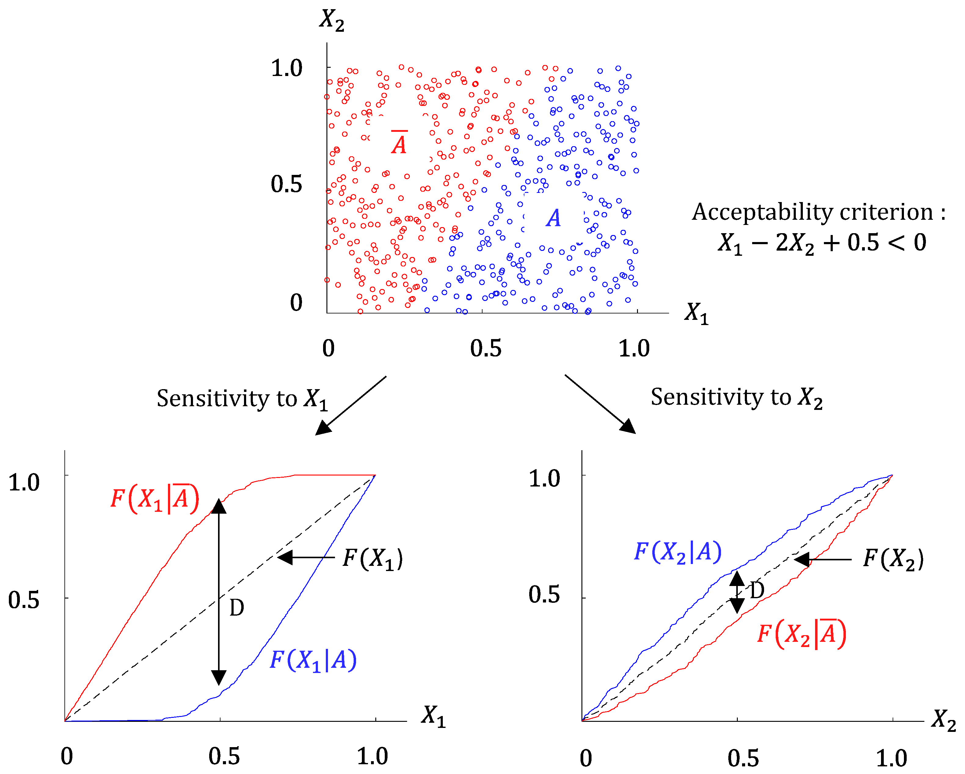
3.5. Regional Sensitivity Analysis

3.5.1. Principle of Regional Sensitivity Analysis

Regional sensitivity analysis (RSA) is a moment-independent method based on Monte Carlo filtering (MCF). This method answers the following questions [15]: which variable or group of variables are influential in leading the model output in a given region of the output space defined by a given acceptability criterion? How does changing an input variable lead to an acceptable or unacceptable realization of the output, according to the acceptability criterion? RSA focuses on the sensitivity of the model in the output region defined by acceptability criterion rather than on the whole output space.

The concept of regional sensitivity analysis based on Monte Carlo filtering was first proposed by Hornberger and Spear in the field of environmental science studies, with dynamic outputs [39,40,41]. It has later been extensively detailed and commented upon in [14].

Let us remind ourselves that we are interested in meeting some targets in the output space (e.g., thresholds and constraint satisfaction). The first step is to state a binary acceptability criterion which defines the desired target (acceptable solutions). Then, like for other sensitivity methods, the input space is sampled and simulations are run for all the sample points. After that, the filtering step consists of checking the ouput acceptability criterion and partitioning the input sample into two subsets: $A$ (acceptable points, for which the model output meets the acceptability criterion) and $\overline{A}$ (non acceptable points, for which the model output does not meet the acceptability criterion). Figure 4 summarizes the MC filtering principle. The respective sizes of $A$ and $\overline{A}$ are denoted by $n$ and $\overline{n}$, and $N=n+\overline{n}$ is the size of the sample and the total number of runs.

The last step is to analyze and interpret the results. If the input variable $X_i$ has no influence on meeting the criterion, then its statistical distribution will be identical within sets $A$ and $\overline{A}$. Hence, in order to detect the influence of the input variable $X_i$ on the compliance with the criterion, we need to compare the statistical distributions of $X_i$ within the $A$ set and the $\overline{A}$ set. These distributions are naturally denoted by $X_i|A$ and $X_i|\overline{A}$. Their empirical cumulative distribution functions, denoted respectively by $F_n\left(X_i|A\right)$ and $F_{\overline{n}}\left(X_i|\overline{A}\right)$, are computed and plotted for each input and then compared. Figure 5 illustrates this principle for a simple example with two input variables. The model is $f\left(X_1,X_2\right)=2X_1-X_2+0.5$, with $X_1$ and $X_2$ uniformly distributed between 0 and 1, while the acceptability criterion is $f\left(X_1,X_2\right)<0$.

Visual comparison between $F_n\left(X_i|A\right)$ and $F_{\overline{n}}\left(X_i|\overline{A}\right)$ gives a global view of the influence of each input variable with respect to the acceptability criterion. The larger the distance between these curves, the larger the influence of $X_i$. Conversely, cumulative distributions that are very close indicate that the input parameter has no influence because the distribution of $X_i$ is the same in the behavioral and the non-behavioral groups.

The shape and the relative positions of the curves also contain information, as illustrated by the example of Figure 5. The fact that $F_n\left(X_2|A\right)$ lies above $F_{\overline{n}}\left(X_2|\overline{A}\right)$ indicates that the criterion is statistically more respected for smaller values of $X_2$: increasing $X_2$ has a negative impact on the respect of the criterion. Conversely, $F_n\left(X_1|A\right)$ lies under $F_{\overline{n}}\left(X_1|\overline{A}\right)$, indicating that increasing $X_1$ has a positive impact. One also notices that $F_n\left(X_1|A\right)$ is zero for $X_1<0.31$. This means that $X_1$ starts to have a positive effect at $X_1=0.31$ (the subset $A$ starts growing). On the other hand, the fact that $F_n\left(X_1|\overline{A}\right)$ reaches 1 at $X_1=0.74$ indicates that no points within $X_1>0.74$ belong to $\overline{A}$, and hence that they are all acceptable. Increasing $X_1$ above $0.74$ has no influence on the respect of the acceptability criterion.

3.5.2. Two-Sample Kolmogorov–Smirnov Test

Visual comparison between the empirical cumulative distribution functions $F_n\left(X_i|A\right)$ and $F_{\overline{n}}\left(X_i|\overline{A}\right)$ provides interesting qualitative information, but a quantitative index is required for a rigorous interpretation of the distance between these curves. Hornberger and Spear proposed using the two-sided Kolmogorov–Smirnov test in order to decide if the two distributions $X_i|A$ and $X_i|\overline{A}$ come from the same continuous distribution or not [39,40,41].

The Kolmogorov–Smirnov test compares the statistical distribution of two samples, based on their empirical distribution functions [64,65,66]. The problem is formulated as follows. Let $\left(x_1, \dots ,x_m\right)$ and $\left(y_1, \dots ,y_n\right)$ be samples of independent observations from random variables with continuous distribution functions $F$ and $G$, and let $F_m$ and $G_n$ be the corresponding empirical distribution function. The null hypothesis H0 to be tested is that $F=G$. The Kolmogorov–Smirnov statistic is defined by:

$$D=su{p}_u\left|F_n\left(u\right)-G_m\left(u\right)\right|$$

Large values of $D$ are significant enough to reject $H0$, but the question is “at what level of significance α does the calculated value of $D$ determines the rejection of H0?”. For a given a priori distance $d$, the significance probability $\alpha$, defined as the probability of rejecting H0 when it is true, is given by:

$$\alpha =Pr(D\ge d | F=G)$$

A large distance $d$ corresponds to a low value of $\alpha$ and a low risk when rejecting H0, i.e., when accepting that $F\ne G$. Conversely, a small distance $d$ corresponds to a higher risk of error when rejecting H0. The relationship between the significance level $\alpha$ and the distance $d$ depends on the sample sizes. If the sample size is large, close forms exist, otherwise tables are used. In practice, the Kolmogorov–Smirnov test is a classical tool available in many programing langages (Mathematica, Matlab, R, Python, Java, Julia, etc.). The user provides the two samples to the Kolmogorov–Smirnov test function and the function returns the distance D and the level of significance associated to it, i.e., the probability of rejecting H0 when it is true.

3.5.3. Practical Implementation and Comments

The different steps for the practical implementation of RSA are as follows:

• Generate a p-input sample that properly covers the input and output spaces and apply the model to calculate the corresponding m-output set. The procedure and the notations are detailed in Section 2.2 and Figure 3. The “rules of art” are the same as for the sensitivity analysis method presented before.
• Classify the sample set into behavioral and non-behavioral subsets $A$ and $\overline{A}$, according to the operational constraints (e.g, pantograph voltages within prescribed limits at all times of simulation).
• For each $X_i$:

  i.

  Sort each subset $A$ and $\overline{A}$ with respect to $X_i$, build and plot the distribution functions $F_n\left(X_i|A\right)$ and $F_{\overline{n}}\left(X_i|\overline{A}\right)$. Proceed to qualitative visual analysis.

  ii.

  Apply the Kolmogorov–Smirnov two-sample test (two-side version) to $F_n\left(X_i|A\right)$ and $F_{\overline{n}}\left(X_i|\overline{A}\right)$ and calculate $D$ and the corresponding significance level $\alpha$.

  iii.

  Categorize $X_i$ as “critical”, “important”, or “insignificant”, according to the significance level $\alpha$ [14]. $X_i$ is said to be a “critical” input if $\alpha$ is below 1%. In other words, the probability of wrongly stating that $X_i|A$ and $X_i|\overline{A}$ are different, and hence that $X_i$ is an influential variable, is less than 1%. An “insignificant” input corresponds to a significance level $\alpha$ above 10%: the risk of wrongly rejecting H0 is deemed too high to conclude about the influence of $X_i$. In between, inputs are categorized as “important”.

Regional sensitivity analysis, based on Monte Carlo filtering and the Kolgomirov–Smirnov test, is an interesting approach to globally characterize the sensitivity of the model to the respect of a given constraint on the output model. This method is conceptually simple and very easy to implement, while the computational cost of the Kolgomirov–Smirnov test is low. Yet, its interpretation requires some precautions [67,68].

Like all statistical methods, it requires a good sampling of the input space, but the fraction of points that meet the behavioral criterion should also be statistically significant.

The Kolgomirov–Smirnov test makes it possible to identify “critical” inputs (the influential ones) and to rank them according to the distance $D$ (the higher $D$ is, the smaller the probability of error). A more delicate point is that one can conclude about the influence of $X_i$ only if H0 is rejected (i.e., if $X_i$ is influential), because the test does not give the probability of wrongly accepting H0. In particular, interaction between input parameters may induce identical $X_i|A$ and $X_i|\overline{A}$ distributions, even if $X_i$ is influential. Hence, it is recommended that researchers complete regional sensitivity analysis alongside other sensitivity analysis indices in order to detect possible interactions between the inputs [67]. Furthermore, it has been reported that the distribution functions tend to be more difficult to interpret when the number of inputs increases.

When properly used, regional sensitivity analysis is a powerful tool [69]. It has been used for various applications (see, for example, [70,71,72]). The authors of [73] present an interesting extension of the filtering principle coupled with optimization, with the partition of the sample into 10 subsets defined by different performance indices.

4. Comparative Analysis

In this section, the three sensitivity analysis methods are applied to a simple test case in order to compare their performances. The power shortage test case is presented and the traffic adjustment problem is specified. Then the influence of the different adjustment actions are established and the results are discussed.

4.1. Test Case Presentation

The test case consists of a 80 km long, 25 kV AC single-track line (Figure 6). The traffic consists of ten high speed trains (TGV) with identical missions (speed setpoints). The line is fed by three substations (SST) and the incident under examination is the loss of the substation located in the middle of the line. The traffic must be rescheduled in order to respect the pantograph voltage operational constraint so that traction engines are operated safely. Specifically, the pantograph voltage must be between 19 kV and 27.5 kV at all times.

In the nominal case, trains depart every five minutes from point pk0. Figure 7 shows the simulation results for the nominal situation. The top curve (a) represents the speed profiles of the ten trains. These curves perfectly overlap because the speed setpoints are the same for all the trains, and therefore the line can transmit enough power to all trains. The bottom curve (b) represents the train catenary voltages, and it is worth some comment. The shape of the voltage curves is correlated with the speed profile. The acceleration phases (for example between pk10 and pk15) correspond to high power demands and result in a drop in the voltage at the catenary. Conversely, during the braking phase (for example between pk58 and pk60), part of the kinetic energy of the train is returned to the line and the voltage rises sharply. The curves do not all overlap because the catenary voltage of each train depends not just on the power drawn by the train itself, but also on that drawn by the other trains traveling along the line. Typically, the catenary voltage of the first train will be higher than the catenary voltage of the following ones. The overall shape of the curves also reflects the position of the supply substations, with a rise in voltage at each substation. The graph does not indicate which train corresponds to each curve, but the important point is that the voltage is always within the desired range (between 19 kV and 27.5 kV).

In the default case, the substation located in the middle of the line is out of order. Figure 8 shows the simulation results for the same traffic as before. Curve (a) shows that the speed profiles of the trains are affected especially between pk40 and pk50, when the trains accelerate just after the faulty substation. The catenary voltages (b) are much lower than in the nominal case and locally drop below the minimum threshold (19 kV). In addition to restricting the power supplied to the trains, this generates significant losses and heating in the cable, and therefore additional operating costs. These results indicate that the electrical network cannot supply the power required by the initial traffic and that the load must be lightened by traffic adjustment actions.

4.2. Adjustment Problem Specification

The first step in rescheduling the traffic is a technical analysis. Based on their expertise and the simulation results, the operator defines traffic adjustment variables as well as the acceptability and performance criteria of the solutions. By doing this, they build an adjustment model, the inputs of which are the adjustment variables and the outputs of which are the physical quantities from which the traffic performance and the constraints are defined.

4.2.1. Adjustment Variables

The comparison of the traffic simulation results in the nominal case and in the degraded case guides the choice of traffic adjustment actions. An initial way to reduce the load on the line is to space the trains apart by increasing the time interval between two successive departures. Furthermore, the voltage and speed profiles indicate that it is between pk40 and pk60 that the train power is the most disturbed. It is therefore useful to study the influence of speed reduction in this part of the line.

The five following adjustment variables have been defined:

-

$X_1 ϵ\left[0,20\right] min$: time interval increase between successive departures;

-

$X_2 ϵ \left[0,20\right] m/s$: speed setpoint reduction between pk40 and pk45;

-

$X_3 ϵ \left[0,20\right] m/s$: speed setpoint reduction between pk45 and pk50;

-

$X_4 ϵ \left[0,20\right] m/s$: speed setpoint reduction between pk50 and pk55;

-

$X_5 ϵ \left[0,20\right] m/s$: speed setpoint reduction between pk55 and pk60.

4.2.2. Outputs and Acceptability Criterion

The acceptability criterion chosen in this study relates to the operational constraint on the catenary voltage. These quantities are the adjustment model outputs. For each train, the sliding 10-second average value must always lie between 19 kV and 27.5 kV. The adjustment model has as many outputs as there are trains, and each output corresponds to a time series. Note that the catenary voltage time series are actually handled as functions of the train positions pk.

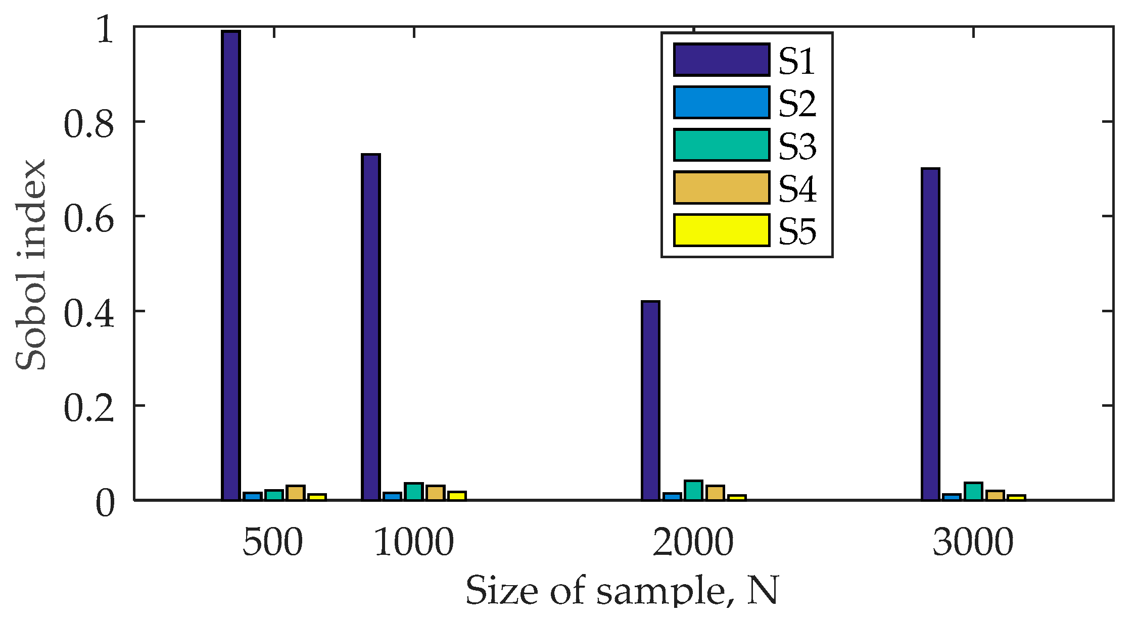
4.3. Generalized Sobol Indices

Generalized first-order Sobol indices were calculated for each of the 10 trains, and for each of the five adjustment variables, for a total of 50 indices.

The Sobol indices computation requires to first build two sampling matrices of dimension $N\times p$, where $N$ is the number of samples and $p$ the number of adjustment variables (here $p=5$). Each row of the matrix corresponds to an adjustment scenario to be tested. Quasi-random sampling is used for a good coverage of the input space. The two sampling matrices are combined as described in Appendix A, and a total of $N\times \left(p+1\right)$ simulations are run. The five Sobol indices ${\left(Si\right)}_{i=1,5}$ are then calculated.

Sobol indices were calculated for an increasing sample size $N$ in order to study the influence of this parameter on the quality of the indices estimate. The memory capacity required for the storage of the outputs necessary for the calculation of the indices did not make it possible to go beyond $N=3000$. Indeed, the catenary voltages must be saved at each pk, for all the trains, and for all simulations. The volume of data to be kept in dynamic memory is proportional to the size of the sample, and ends up saturating the RAM of the computer. Details will be given in Section 4.6.

The results are shown in Figure 9. As results are very similar for the different trains, only the indices corresponding to train no. 3 are presented here. It can be seen that even with $N=3000$, the sensitivity indices do not seem to have reached convergence. However, despite the estimation error, the variable $X_1$ (time delay between trains) appears to have a preponderant influence over the other variables (speed reductions). Among the speed reductions, the variable $X_3$ seems to stand out a bit from the others, although one would expect $X_2$ to be more influential, since it acts closer to the faulty substation, in a region where the speed and the voltage appear to be strongly affected.

4.4. Energy Distance-Based Indices

The energy distance approach was applied to calculate another series of sensitivity indices related to the input X_i. Figure 10 shows the results for an increasing sample size. As before, these indices are related to train no. 3. The same trends are observed, with the dominant influence of $X_1$. The ranking between the speed reductions ($X_2$ to $X_5$) better corresponds to what is intuitively expected.

This method requires only one $N\times p$ sample matrix and $N$ evaluations of the model instead of $6N$ for Sobol indices, which is a significant gain.

Figure 10 shows that this method has a fast convergence, with significant results from a sample size of 500. The gain is obvious compared to the Sobol method. However, the computation time of the indices themselves (in the post-processing phase) increases rapidly with the number of adjustment variables. If the method is applied to a very fast model, the conclusion may be more balanced.

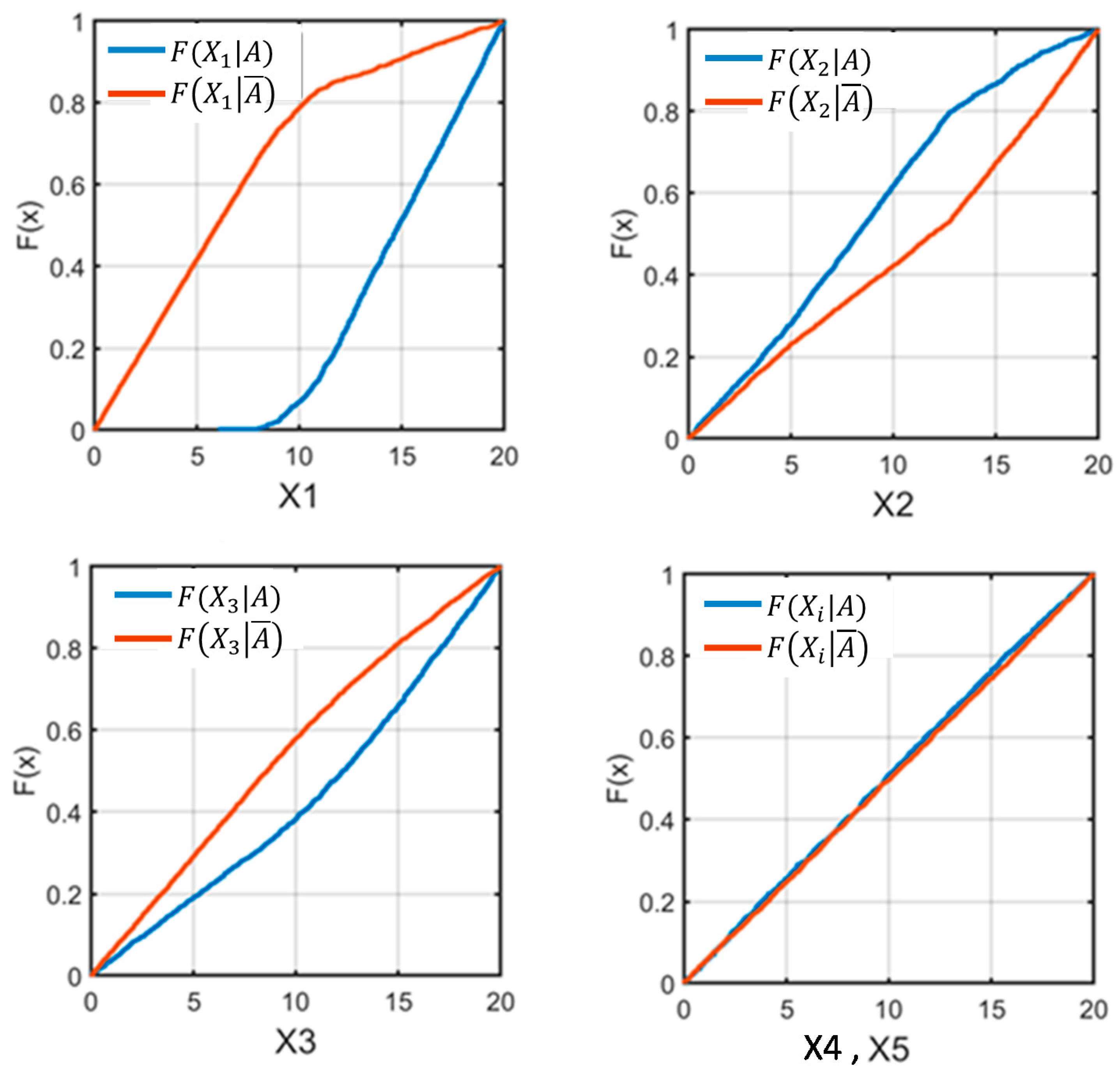
4.5. Regional Sensitivity Analysis

The last method tested, regional sensitivity analysis, focuses on the influence of the adjustment variables in relation to the catenary voltage constraint. This voltage must remain between 19 kV and 27.5 kV throughout the journey of all trains.

This method requires an $N\times p$ sample matrix and $N$ evaluations of the model. The sample matrix is partitioned into two groups, denoted by $A$ and $\overline{A}$, depending on whether the constraint on the voltage output is satisfied or not. For each input $X_i$, the empirical cumulative densities of both groups, denoted respectively by $F\left(X_i|A\right)$ and $F\left(X_i|\overline{A}\right)$, are computed. Figure 11 shows the graphs of the functions $F\left(X_i|A\right)$ (blue curve) and $F\left(X_i|\overline{A}\right)$ (red curve) for the five input variables. These curves are calculated for a sample size of $N=1000$.

Visual comparison between $F\left(X_i|A\right)$ and $F\left(X_i|\overline{A}\right)$ gives a global overview of the influence of each input variable: the greater the difference between between $F\left(X_i|A\right)$ and $F\left(X_i|\overline{A}\right)$, the greater the influence of $X_i$. Again, $X_1$ is found to be the most influential variable, whereas $X_4$ and $X_5$ do not show any influence.

Other interesting information is provided by these curves. For $X_1$, the shape of $F\left(X_1|A\right)$ (plot (a), blue curve) indicate that no sample with $X_1<8mn$ respects the voltage constraint. The graphs also show that the variables $X_1$ and $X_3$ have a positive influence on the output: increasing them increases compliance with the catenary voltage constraint. On the contrary, the variable $X_2$ is found to have a negative influence: reducing the speed on the 40–45 km section is not favorable. This non-intuitive result is due to the fact that this speed reduction causes trains to get closer to each other in a section of line where the power supply is low.

The two-sample Kolmogorov–Smirnov test provides a statistical interpretation of the distance between $F\left(X_i|A\right)$ and $F\left(X_i|\overline{A}\right)$. Figure 12 plots the statistic $D$ as a function of the sample size $N$ and quantifies the qualitative observations made in the previous paragraph.

Table 1. Significance level $\alpha$ for the different input variables and sample sizes.

Sample Size N	${\mathit{\alpha }}_{{\mathbf{X}}_1}$	${\mathit{\alpha }}_{{\mathbf{X}}_2}$	${\mathit{\alpha }}_{{\mathbf{X}}_3}$	${\mathit{\alpha }}_{{\mathbf{X}}_4}$	${\mathit{\alpha }}_{{\mathbf{X}}_5}$
100	0.0	0.05	0.09	0.59	0.7
500	0.0	0.0	0.0	1.0	0.99
1000	0.0	0.0	0.0	1.0	1.0
2000	0.0	0.0	0.0	0.98	1.0
3000	0.0	0.0	0.0	0.7	1.0
4000	0.0	0.0	0.0	0.57	1.0
Class	critical	critical	critical	insignificant	insignificant

reports the corresponding values of statistical significance $\alpha$, also called the p-Value, and classifies the variables $X_1$, $X_2$, and $X_3$ as critical ($\alpha <0.01$) and the variables $X_4$ and $X_5$ as insignificant ($\alpha >0.1$).

Regional sensitivity analysis requires an $N\times p$ sample matrix and $N$ evaluations of the model, like the energy distance method. However, the post-processing of the simulation results and the indices computation is much faster and requires less memory. Furthermore, the convergence is satisfactory, provided that there are enough points in each subset $A$ and $\overline{A}$.

4.6. Assessment and Comparison of the Tested Methods

Regardless of the sensitivity analysis method used, the conclusion is the same. Train spacing always appears to be a much more influential variable than the others. As might be expected, speed reductions are more influential the closer they are to the faulty substation. The small influence of the train speed reduction parameter is explained by the fact that this reduction does not change the acceleration of the trains, but the duration of the acceleration phase. Therefore, it does not affect the load peaks and the voltage drop due to acceleration, but their duration.

The three methods are now compared on the following criteria: overall calculation time (model and indices computation), memory space required to store the data needed for the indices calculation, and convergence speed. The convergence speed corresponds to the sample size $N$ required to obtain a good statistical estimate of the sensitivity indices (i.e., the point at which adding samples no longer creates a significant variation on the calculated indices).

Table 2. Computation cost of the tested methods.

	N = 500		N = 1000
	Time (Min)	Memory (MB)	Time (Min)	Memory (MB)
Sobol	256	495	901	907
Energy distance	40	340	150	611
Regional	35	280	121	547

compares the computation cost of the three tested methods. The computation was performed on a laptop with the following specifications: DELL Latitude 7480, CPU: Intel Core i7-7600U (2 cores/4 threads/4 MB cache/2.8 GHz), RAM: 16 GB.

Sobol indices computation requires $N\left(p+1\right)$ calls to the simulator, i.e., $6N$ calls in the present case. Moreover, convergence requires a larger number of samples. The other two methods require only $N$ calls to the model and convergence is therefore faster. For the considered problem, for $N=1000$, it takes 15 hours to calculate the Sobol indices, for an imprecise result, while 2 hours are enough for a good result with the other methods.

Table 3. Performances and specificity of the different methods.

	Calculation Time	Convergence Speed	Storage Space	Specificity
Generalized Sobol	High	Slow	High	Can characterize interaction
Energy distance	Average	Fast	Average	Moment independant
Regional analysis	Low	Average	Low	Based on acceptability criterion

summarizes the performances and the specificity of the three sensitivity analysis methods under examination. This criteria are intended to generalize the conclusions of the present study and guide the choice of the sensitivity analysis method best suited to a given problem.

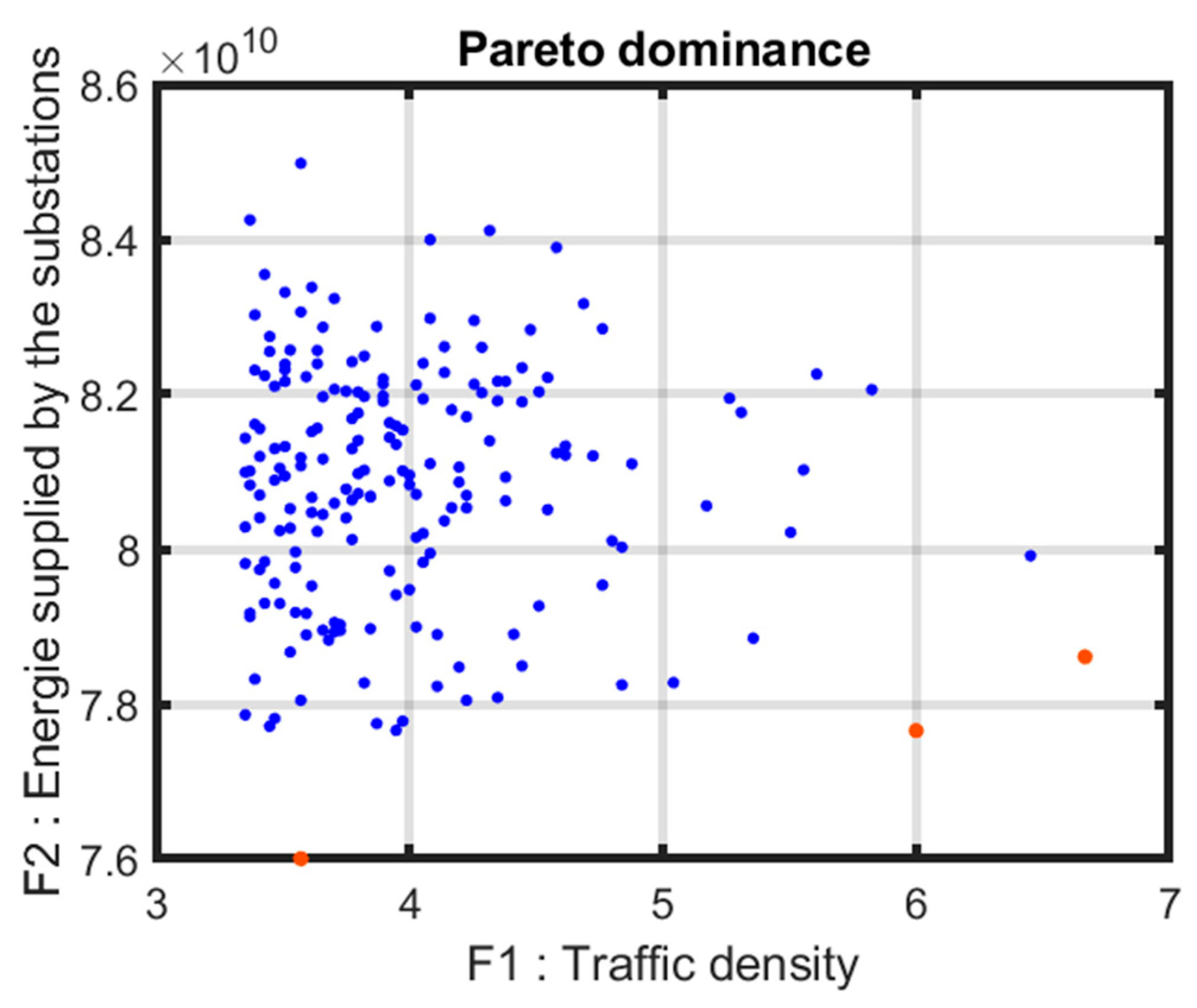
4.7. Empirical Pareto Set

When conducting a sensitivity analysis, one actually runs Monte Carlo simulations with a wide coverage of the input space. Hence, it is natural to exploit these results to build empirical Pareto plots.

In this section, the simulation results are processed in order to find optimal solutions among the acceptable solutions generated from the regional sensitivity method. Two cost functions are considered:

• F1: traffic density.
• F2: total energy supplied by the substations.

F1 should be maximized, whereas F2 should be minimized, and so the objectives are contradictory. Figure 13 shows the empirical Pareto plot. Each dot represents an acceptable solution. Blue dots represent dominated solutions and red dots represent compromised solutions. This plot shows that increasing the traffic density also increases the total energy consumed by the traffic. This is due to the increasing part played by losses.

5. Application to a Real Case

The comparison made in Section 4 shows that regional sensitivity analysis is the most suitable method for our traffic rescheduling problem. In the present section, a test case representative of a real study is considered. The network has several branches, and many different types of trains travel back and forth. This example is intended to assess the capability of the proposed methodology to highlight efficient rescheduling actions and provide objective information to the decision maker.

5.1. Test Case Description

The test case corresponds to a suburban railway network in the Paris region. The traffic consists of more than 300 trains with various missions. Figure 14 shows the network topology. The power supply system is in 1500 V DC mode, with 83 feeding substations. The study deals with the loss of the substation "GRIAULT" on Line 5. The catenary voltage must remain between 1750 V and 1000 V.

Simulations were run in for the nominal case (Griault substation operational) and the degraded case (Griault substation out of order). Figure 15 and Figure 16 show the speed profiles of the trains along Line 5, and the corresponding catenary voltage profile. In the degraded case, trains are slowed down between the positions at 60 and 70 km, and the catenary voltage drops locally below the minimum threshold (1000 V). This indicates that the electrical network cannot provide the power necessary to achieve the speed instructions on Line 5 and that the traffic must be adjusted.

5.2. Rescheduling Process

The principle of adjustment actions is simple to state, but more delicate to implement because of the heterogeneity of traffic and the multiplicity of lines and tracks. In practice, the trains are gathered into groups and subgroups, according to common characteristics: line, track, type of train, departure point, etc. For the present situation, six adjustment actions were defined by the operator in charge of rescheduling the traffic:

• Delete comfort auxiliaries for suburb trains, type 1;
• Delete comfort auxiliaries for suburb trains, type 2;
• Space the consecutive trains of group G1;
• Space the consecutive trains of group G2;
• Space the consecutive trains of group G3;
• Space the consecutive trains of group G6.

Each adjustment is modeled by a variable in a range of variation chosen by the operator. A sample of $N=400$ scenarios was drawn and corresponding simulations were run, for a total computation time of 4 hours. A subset of 311 scenarios were found to respect the operational constraint on the catenary voltage (acceptable solutions).

Table 4. Results of regional sensitivity analysis.

Adjustment	Distance D	Significance Level α	Class
Adjustment 1	0.34	0.0	Critical
Adjustment 2	0.04	1	Insignificant
Adjustment 3	0.08	0.63	Insignificant
Adjustment 4	0.1	0.37	Insignificant
Adjustment 5	0.27	0.0	Critical
Adjustment 6	0.6	0.0	Critical

gives the results of the regional sensitivity analysis. Among the six actions, three are found to be critical (adjustment 1, adjustment 5 and adjustment 6).

$\mathrm{Significance}$ Among the 400 tested solutions, the acceptable solution with the highest train density (335 against 346 in the initial case) and the lowest energy consumption was adjustment 3, which is considered as the best one. This solution corresponds to the following transport plan:

• Delete comfort auxiliaries for suburb trains, type 1: yes;
• Delete comfort auxiliaries for suburb trains, type 2: yes;
• Space the consecutive trains of group G1: 4 minutes;
• Space the consecutive trains of group G2: 1 minute;
• Space the consecutive trains of group G3: 11 minutes;
• Space the consecutive trains of group G6: 2 minutes.

The next step is to refine the analysis in the vicinity of the best solution. For this step, all non-important adjustments in the reorganization process are removed and set to zero, and a random sample of only 40 scenarios is considered. As a results, the best solution corresponds to a train density of 345.

5.3. Conclusions

This test case is representative of a real rescheduling problem that SNCF Réseau has had to handle. The formalization of the problem and the use of regional sensitivity anaslysis provide objective indicators to guide the operator in charge of the rescheduling process and simplify the optimization problem. In this test, the optimization criterion is the traffic density, but the operator can choose another criterion or multi-criteria. The execution time of the research process depends on the size of the studied area and the size of the sample. SNCF Réseau is currently integrating this method into its numerical toolset for the resolution of incident, either for real-time or upstream studies.

6. Conclusions

Railway networks are complex systems and their analysis relies on heavy simulations. In the event of electrical equipment failure, the power that can be delivered to the trains is restricted and the traffic should be optimally rescheduled within the physical limits of the power system. Namely, traffic adjustment actions, such as train spacing or train slowing must be assessed, so that the train supply voltage never drops below a critical value given by technical standards. This rescheduling task is an important decision-making process for the smooth operation of the network, and it requires a complete and accurate physical simulation (no assumptions can be made).

The studied system is a complex one, with nonlinear behavior, a large number of input and output variables, and a computationally intensive simulation code. Furthermore, the output variables are large time series. As direct optimization is too difficult, we propose performing sensitivity analysis in order to identify the most influential traffic adjustement variables and drop the variables with negligible influence.

A review of sensitivity analysis methods has been conducted, and three global sensitivity analysis methods suitable for black box, multivariate, nonlinear models have been identified: generalized Sobol indices, energy distance-based indices, and regional sensitivity analysis. The three methods have been described, applied to a simple traffic rescheduling test case, and their performances have been compared. The conclusions are as follows:

• Variance-based method: Sobol indices are sensitivity indices based on the output variance. They are widespread for scalar outputs and have been generalized for vector outputs, such as time series. Second order indices can provide information about the interactions between inputs, but usually only the first-order indices are calculated. The computation of Sobol indices requires large samples in order to reach convergence, and, furthermore, the number of model evaluations is proportional to the number of tested inputs. Hence, the computation time may become prohibitive in the case of numerically intensive models.
• Energy distance-based method: The energy distance is used to quantify the distance between the output $Y$ and the conditional distributions $Y|X_i$ over the whole domain. This distance facilitates the definition of normalized sensitivity. The method was initially proposed for scalar outputs, but it naturally generalizes to series outputs. As this method is moment independent, it is more general than Sobol indices. Furthermore, its computation cost is significantly lower because of faster convergence of the estimates and because the number of model evaluations does not depend on the number of input variables.
• Regional sensitivity analysis: This method applies to problems involving an acceptability criterion on the output, and tests the influence of the input variables in respect to this criterion. So-called Monte Carlo filtering is used to partition the input space into an acceptable set and a non-acceptable set. Then the two sets are compared statistically in order to highlight the influence of each input variable. This method is the fastest and the easiest one to implement.
• The results of the three methods are consistent: they lead to the same input ranking of the input, but the cost of Sobol indices is much higher than the two other methods. Regional sensitivity analysis appears to be the most suitable method for the present application: it is relatively easy to implement, rather fast, and accounts for constraints on the system output, a key feature for electrical incident management.

Hence, regional sensitivity analysis has been applied to a test case representative of a real rescheduling problem. The results show which traffic adjustment actions are the most efficient for keeping the catenary voltage within the prescribed limits. Subsequently, the actions that are not important can be frozen for a simplified optimization. The proposed approach provides objective information for rescheduling traffic in an efficient way and is a useful tool to guide the traffic manager.

The sensitivity analysis methods that have been described in the present paper can be applied to any problem with the same characteristics; i.e., nonlinear, black box models with multivariate outputs (and possibly constraints on the outputs). Such problems are to be encountered in the design of optimal power systems involving temporal or spatial outputs, heavy models, and/or constraints on the outputs. It can be applied for sizing power systems (electrical machines and regulators). For example, one may think of battery sizing and management problems in hybrid systems, or electrical vehicle systems in their environment (e.g., regulation or driving cycles).

References

1. Cacchiani, V.; Huisman, D.; Kidd, M.; Kroon, L.; Toth, P.; Veelenturf, L.; Wagenaar, J. An overview of recovery models and algorithms for real-time railway rescheduling. Transp. Res. Part B Methodol. 2014, 63, 15–37. [Google Scholar] [CrossRef] [Green Version]
2. Krasemann, J. Greedy algorithm for railway traffic re-scheduling during disturbances: A Swedish case. IET Intell. Transp. Syst. 2010, 4, 375–386. [Google Scholar] [CrossRef] [Green Version]
3. Dündar, S.; Şahin, I. Train re-scheduling with genetic algorithms and artificial neural networks for single-track railways. Transp. Res. Part C Emerg. Technol. 2013, 27, 1–15. [Google Scholar] [CrossRef]
4. Schachtebeck, M.; Schöbel, A. To Wait or Not to Wait—And Who Goes First? Delay Management with Priority Decisions. Transp. Sci. 2010, 44, 307–321. [Google Scholar] [CrossRef]
5. D’Ariano, A.; Pacciarelli, D.; Sama, M.; Corman, F. Microscopic delay management: Minimizing train delays and passenger travel times during real-time railway traffic control. In Proceedings of the 2017 5th IEEE International Conference on Models and Technologies for Intelligent Transportation Systems (MT-ITS), Naples, Italy, 26–28 June 2017; pp. 309–314. [Google Scholar]
6. Louwerse, I.; Huisman, D. Adjusting a railway timetable in case of partial or complete blockades. Eur. J. Oper. Res. 2014, 235, 583–593. [Google Scholar] [CrossRef] [Green Version]
7. Ghaemi, N.; Goverde, R.; Cats, O. Railway disruption timetable: Short-turnings in case of complete blockage. In Proceedings of the 2016 IEEE International Conference on Intelligent Rail Transportation (ICIRT), Birmingham, UK, 23–25 August 2016; pp. 210–218. [Google Scholar]
8. Zhan, S.; Kroon, L.G.; Veelenturf, L.P.; Wagenaar, J.C. Real-time high-speed train rescheduling in case of a complete blockage. Transp. Res. Part B Methodol. 2015, 78, 182–201. [Google Scholar] [CrossRef]
9. Narayanaswami, S.; Rangaraj, N. Modelling disruptions and resolving conflicts optimally in a railway schedule. Comput. Ind. Eng. 2013, 64, 469–481. [Google Scholar] [CrossRef]
10. Binder, S.; Maknoon, Y.; Bierlaire, M. The multi-objective railway timetable rescheduling problem. Transp. Res. Part C Emerg. Technol. 2017, 78, 78–94. [Google Scholar] [CrossRef] [Green Version]
11. Lusby, R.M.; Larsen, J.; Ehrgott, M.; Ryan, D. Railway track allocation: Models and methods. OR Spectr. 2011, 33, 843–883. [Google Scholar] [CrossRef]
12. Cacchiani, V.; Toth, P. Nominal and robust train timetabling problems. Eur. J. Oper. Res. 2012, 219, 727–737. [Google Scholar] [CrossRef]
13. Desjouis, B.; Remy, G.; Ossart, F.; Marchand, C.; Bigeon, J.; Sourdille, E. A new generic problem formulation dedicated to electrified railway systems. In Proceedings of the 2015 International Conference on Electrical Systems for Aircraft, Railway, Ship Propulsion and Road Vehicles (ESARS), Aachen, Germany, 3–5 March 2015; pp. 1–6. [Google Scholar] [CrossRef] [Green Version]
14. Saltelli, A. (Ed.) Sensitivity Analysis in Practice: A Guide to Assessing Scientific Models; Wiley: Hoboken, NJ, USA, 2004. [Google Scholar]
15. Saltelli, A.; Ratto, M.; Andres, T.; Campolongo, F.; Cariboni, J.; Gatelli, D.; Saisana, M.; Tarantola, S. Global Sensitivity Analysis: The Primer; Wiley: Hoboken, NJ, USA, 2008. [Google Scholar]
16. Iooss, B.; Lemaître, P. A review on global sensitivity analysis methods. In Uncertainty Management in Simulation-Optimization of Complex Systems; Springer: Boston, MA, USA; Available online: http://arxiv.org/abs/1404.2405 (accessed on 3 June 2021).
17. Becker, W.; Paruolo, P.; Saisana, M.; Salkelli, A. Weights and importance in composite indicators: Mind the gap. In Handbook of Uncertainty Quantification; Ghanem, R., Higdon, D., Owhadi, H., Eds.; Springer International Publishing: Cham, Switzerland, 2017; pp. 1187–1216. [Google Scholar] [CrossRef]
18. Morio, J. Global and local sensitivity analysis methods for a physical system. Eur. J. Phys. 2011, 32, 1577–1583. [Google Scholar] [CrossRef]
19. Morris, M.D. Factorial Sampling Plans for Preliminary Computational Experiments. Technometrics 1991, 33, 161. [Google Scholar] [CrossRef]
20. Saltelli, A.; Ratto, M.; Tarantola, S.; Campolongo, F. Sensitivity analysis practices: Strategies for model-based inference. Reliab. Eng. Syst. Saf. 2006, 91, 1109–1125. [Google Scholar] [CrossRef]
21. Sobol’, I.M. Sensitivity estimates for nonlinear mathematical models (translated from Russian). Math. Model. Comput. Exp. 1993, 1, 407–414. [Google Scholar]
22. Sobol′, I.M. Global sensitivity indices for nonlinear mathematical models and their Monte Carlo estimates. Math. Comput. Simul. 2001, 55, 271–280. [Google Scholar] [CrossRef]
23. Sobol, I.M.; Kucherenko, S.S. Global sensitivity indices for nonlinear mathematical models. Review. Wilmott 2005, 2005, 56–61. [Google Scholar] [CrossRef]
24. Reuter, U.; Liebscher, M. Global Sensitivity Analysis in View of Nonlinear Structural Behavior; LS-DYNA: Anwenderforum, Bamberg, 2008. [Google Scholar]
25. Bolado-Lavin, R.; Castaings, W.; Tarantola, S. Contribution to the sample mean plot for graphical and numerical sensitivity analysis. Reliab. Eng. Syst. Saf. 2009, 94, 1041–1049. [Google Scholar] [CrossRef]
26. Tarantola, S.; Kopustinskas, V.; Bolado-Lavin, R.; Kaliatka, A.; Ušpuras, E.; Vaišnoras, M. Sensitivity analysis using contribution to sample variance plot: Application to a water hammer model. Reliab. Eng. Syst. Saf. 2012, 99, 62–73. [Google Scholar] [CrossRef]
27. Harris, T.; Yu, W. Variance decompositions of nonlinear-dynamic stochastic systems. J. Process. Control. 2010, 20, 195–205. [Google Scholar] [CrossRef]
28. Li, L.; Lu, Z. Regional importance effect analysis of the input variables on failure probability and its state dependent parameter estimation. Comput. Math. Appl. 2013, 66, 2075–2091. [Google Scholar] [CrossRef]
29. Campbell, K.; McKay, M.D.; Williams, B.J. Sensitivity analysis when model outputs are functions. Reliab. Eng. Syst. Saf. 2006, 91, 1468–1472. [Google Scholar] [CrossRef]
30. Garcia-Cabrejo, O.; Valocchi, A. Global Sensitivity Analysis for multivariate output using Polynomial Chaos Expansion. Reliab. Eng. Syst. Saf. 2014, 126, 25–36. [Google Scholar] [CrossRef]
31. Lamboni, M.; Makowski, D.; Lehuger, S.; Gabrielle, B.; Monod, H. Multivariate global sensitivity analysis for dynamic crop models. Field Crop. Res. 2009, 113, 312–320. [Google Scholar] [CrossRef]
32. Lamboni, M.; Monod, H.; Makowski, D. Multivariate sensitivity analysis to measure global contribution of input factors in dynamic models. Reliab. Eng. Syst. Saf. 2011, 96, 450–459. [Google Scholar] [CrossRef]
33. Gamboa, F.; Janon, A.; Klein, T.; Lagnoux, A. Sensitivity indices for multivariate outputs. Comptes Rendus Math. 2013, 351, 307–310. [Google Scholar] [CrossRef] [Green Version]
34. Gamboa, F.; Janon, A.; Klein, T.; Lagnoux, A. Sensitivity analysis for multidimensional and functional outputs. Electron. J. Stat. 2014, 8, 575–603. [Google Scholar] [CrossRef]
35. Lijie, C.; Bo, R.; Ze, L. Importance measures of basic variable under multiple failure modes and their solutions. In Proceedings of the 2016 IEEE Chinese Guidance, Navigation and Control Conference (CGNCC), Nanjing, China, 12–14 August 2016; pp. 1605–1611. [Google Scholar]
36. Greegar, G.; Manohar, C. Global response sensitivity analysis using probability distance measures and generalization of Sobol’s analysis. Probabilit. Eng. Mech. 2015, 41, 21–33. [Google Scholar] [CrossRef]
37. Pianosi, F.; Wagener, T. A simple and efficient method for global sensitivity analysis based on cumulative distribution functions. Environ. Model. Softw. 2015, 67, 1–11. [Google Scholar] [CrossRef] [Green Version]
38. Rizzo, M.L.; Székely, G.J. Energy distance. Wiley Interdiscip. Rev. Comput. Stat. 2015, 8, 27–38. [Google Scholar] [CrossRef]
39. Hornberger, G. Eutrophication in peel inlet—I. The problem-defining behavior and a mathematical model for the phosphorus scenario. Water Res. 1980, 14, 29–42. [Google Scholar] [CrossRef]
40. Spear, R. Eutrophication in peel inlet—II. Identification of critical uncertainties via generalized sensitivity analysis. Water Res. 1980, 14, 43–49. [Google Scholar] [CrossRef]
41. Hornberger, G.M.; Spear, R.C. Approach to the preliminary analysis of environmental systems. J. Environ. Manag. 1981, 12, 7–18. [Google Scholar]
42. Stratified Sampling—Research Methodology. Available online: https://research-methodology.net/sampling-in-primary-data-collection/stratified-sampling (accessed on 14 August 2021).
43. McKay, M.D.; Beckman, R.J.; Conover, W.J. A Comparison of Three Methods for Selecting Values of Input Variables in the Analysis of Output from a Computer Code. Technometrics 2000, 42, 55–61. [Google Scholar] [CrossRef]
44. Helton, J.; Davis, F. Latin hypercube sampling and the propagation of uncertainty in analyses of complex systems. Reliab. Eng. Syst. Saf. 2003, 81, 23–69. [Google Scholar] [CrossRef] [Green Version]
45. Sobol’, I.; Levitan, Y. A pseudo-random number generator for personal computers. Comput. Math. Appl. 1999, 37, 33–40. [Google Scholar] [CrossRef] [Green Version]
46. Yang, H. Quasi Random Sampling for Operations Management. Seoul J. Bus. 2006, 12, 53–72. [Google Scholar]
47. Burhenne, S.; Jacob, D.; Henze, P.G. Sampling based on Sobol sequences for Monte Carlo techniques applied to building simulations. In Proceedings of the 12th Conference of the International Building Performance Simulation Association, Sydney, Australia, 14–16 November 2011; pp. 1816–1823. [Google Scholar]
48. Bratley, P.; Fox, B.L. Algorithm 659. ACM Trans. Math. Softw. 1988, 14, 88–100. [Google Scholar] [CrossRef]
49. Dalal, I.L.; Stefan, D.; Harwayne-Gidansky, J. Low discrepancy sequences for Monte Carlo simulations on reconfigurable platforms. In Proceedings of the 2008 International Conference on Application-Specific Systems, Architectures and Processors, Leuven, Belgium, 2–4 July 2008; pp. 108–113. [Google Scholar]
50. Sobol Quasirandom Point Set—MATLAB. Available online: https://www.mathworks.com/help/stats/sobolset.html (accessed on 9 June 2021).
51. GitHub—Stevengj/Sobol.jl: Generation of Sobol Low-Discrepancy Sequence (LDS) for the Julia Language. Available online: https://github.com/stevengj/Sobol.jl (accessed on 9 June 2021).
52. Homma, T.; Saltelli, A. Importance measures in global sensitivity analysis of nonlinear models. Reliab. Eng. Syst. Saf. 1996, 52, 1–17. [Google Scholar] [CrossRef]
53. Saltelli, A.; Annoni, P.; Azzini, I.; Campolongo, F.; Ratto, M.; Tarantola, S. Variance based sensitivity analysis of model output. Design and estimator for the total sensitivity index. Comput. Phys. Commun. 2010, 181, 259–270. [Google Scholar] [CrossRef]
54. Hoeffding, W. A Class of Statistics with Asymptotically Normal Distribution. Ann. Math. Stat. 1948, 19, 293–325. [Google Scholar] [CrossRef]
55. Dimov, I.; Georgieva, R. Monte Carlo algorithms for evaluating Sobol’ sensitivity indices. Math. Comput. Simul. 2010, 81, 506–514. [Google Scholar] [CrossRef]
56. Owen, A.B. Variance Components and Generalized Sobol’ Indices. SIAM/ASA J. Uncertain. Quantif. 2013, 1, 19–41. [Google Scholar] [CrossRef] [Green Version]
57. Székely, G.J.; Rizzo, M.L. Energy statistics: A class of statistics based on distances. J. Stat. Plan. Inference 2013, 143, 1249–1272. [Google Scholar] [CrossRef]
58. Székely, G.J.; Rizzo, M.L. A new test for multivariate normality. J. Multivar. Anal. 2005, 93, 58–80. [Google Scholar] [CrossRef] [Green Version]
59. Xiao, S.; Lu, Z.; Wang, P. Multivariate global sensitivity analysis for dynamic models based on energy distance. Struct. Multidiscip. Optim. 2017, 57, 279–291. [Google Scholar] [CrossRef]
60. Borgonovo, E. A new uncertainty importance measure. Reliab. Eng. Syst. Saf. 2007, 92, 771–784. [Google Scholar] [CrossRef]
61. Plischke, E.; Borgonovo, E.; Smith, C. Global sensitivity measures from given data. Eur. J. Oper. Res. 2013, 226, 536–550. [Google Scholar] [CrossRef]
62. Borgonovo, E.; Hazen, G.B.; Plischke, E. A Common Rationale for Global Sensitivity Measures and Their Estimation. Risk Anal. 2016, 36, 1871–1895. [Google Scholar] [CrossRef] [PubMed]
63. Li, L.; Lu, Z.; Wu, D. A new kind of sensitivity index for multivariate output. Reliab. Eng. Syst. Saf. 2016, 147, 123–131. [Google Scholar] [CrossRef]
64. Massey, F.J. The Kolmogorov-Smirnov Test for Goodness of Fit. J. Am. Stat. Assoc. 1951, 46, 68. [Google Scholar] [CrossRef]
65. Hodges, J.L. The significance probability of the smirnov two-sample test. Arkiv Matematik 1958, 3, 469–486. [Google Scholar] [CrossRef]
66. Ferignac, P. Test de Kolmogorov-Smirnov sur la validité d’une fonction de distribution. Rev. Stat. Appl. 1962, 10, 13–32. [Google Scholar]
67. Spear, R.C.; Grieb, T.M.; Shang, N. Parameter uncertainty and interaction in complex environmental models. Water Resour. Res. 1994, 30, 3159–3169. [Google Scholar] [CrossRef]
68. Ratto, M.; Pagano, A.; Young, P. Factor Mapping and Metamodeling; JCR Scientific and Technical Reports; Joint Research Centre: Ispra, Italy, 2007. [Google Scholar]
69. Borgonovo, E.; Plischke, E. Sensitivity analysis: A review of recent advances. Eur. J. Oper. Res. 2016, 248, 869–887. [Google Scholar] [CrossRef]
70. Wu, Z.; Yang, X.; Sun, X. Application of Monte Carlo filtering method in regional sensitivity analysis of AASHTOWare Pavement ME design. J. Traffic Transp. Eng. 2017, 4, 185–197. [Google Scholar] [CrossRef]
71. Sieber, A.; Uhlenbrook, S. Sensitivity analyses of a distributed catchment model to verify the model structure. J. Hydrol. 2005, 310, 216–235. [Google Scholar] [CrossRef]
72. Brockmann, D.; Morgenroth, E. Evaluating operating conditions for outcompeting nitrite oxidizers and maintaining partial nitrification in biofilm systems using biofilm modeling and Monte Carlo filtering. Water Res. 2010, 44, 1995–2009. [Google Scholar] [CrossRef]
73. Wagener, T.; Lees, M.J.; Wheater, H.S. A toolkit for the development and application of parsimonious hydrological models. In Mathematical Models of Small Watershed Hydrology; Water Resources Publications: Littleton, CO, USA, 2001; Volume 2, p. 34. [Google Scholar]
Figure 1. Railway simulator ESMERALDA NG.
Energies 14 06420 g001
Figure 2. Principle of the adjustment model.
Energies 14 06420 g002
Figure 3. Sampling phase and notations.
Energies 14 06420 g003
Figure 4. Monte Carlo filtering: the model is applied to the input sample and the acceptability criteron is checked. Then, the input sample is partitioned into the acceptable subset A (blue points, whose outputs meet the acceptability criterion), and the non acceptable subset A ¯ (red points, whose outputs do not meet the acceptability criterion).
Energies 14 06420 g004
Figure 5. A simple example of Monte Carlo filtering and the resulting conditional distributions. The large distance between F ( X 1 | A ) and F ( X 1 | A ¯ ) indicate a high sensitivity to X 1 , especially around X 1 = 0.5 .
Energies 14 06420 g005
Figure 6. Position of the feeding substations (SST) along the test case line. The substation at 40 km is out of order. The variables X1 to X5 model the traffic adjustment actions (see Section 4.2.1). X1 is the increase of time between successive train departures, whereas X2 to X5 are speed reductions along different line segments.
Energies 14 06420 g006
Figure 7. Simulation results for the nominal case: (a) speed profiles (10 overlapping curves); (b) catenary voltage. The voltage must remain between the lower limit (19 kV, red continuous line) and the upper limit (27.5 kV, red dashed line).
Energies 14 06420 g007
Figure 8. Simulation results for the degraded case: (a) speed profiles, showing that the speed of the trains is affected between pk = 40 km and pk = 50 km; (b) catenary voltage. The red continuous line represent the lower limit (19 kV) and the red dashed line represents the upper limit (27.5 kV). The voltage locally drops below 19 kV (red ellipse).
Energies 14 06420 g008
Figure 9. Sobol indices S i versus sample size N .
Energies 14 06420 g009
Figure 10. Energy-based sensitivity indices versus sample size N .
Energies 14 06420 g010
Figure 11. Cumulated density functions FXi|A and FXi|A for each input Xi.
Energies 14 06420 g011
Figure 12. D-stat values versus sample size N.
Energies 14 06420 g012
Figure 13. Empirical Pareto plot. Each dot represents an acceptable solution. Blue dots represent dominated solutions and red dots represent compromised solutions.
Energies 14 06420 g013
Figure 14. Topology and electric configuration of the test case. Each color corresponds to a train line. The red square locates the default substation.
Energies 14 06420 g014
Figure 15. Simulation results in the nominal situation: (a) speed; (b) catenary voltage of the trains on line 5.
Energies 14 06420 g015
Figure 16. Results in the degraded situation, before adjustment: (a) speed; (b) catenary voltage of the trains on Line 5.
Energies 14 06420 g016