Development and Analysis of a Dynamic Energy Model of an Office Using a Building Management System (BMS) and Actual Measurement Data

Abstract

Calibration of the energy model of a building is one of the essential tasks required to determine the efficiency of building management systems, and both their own and other systems’ improvement potential. In order to make the building energy model as accurate as possible, it is necessary to collect comprehensive data on its operation and sometimes to assess the missing information. This paper represents the process of developing an energy model for an administrative building and its calibration procedure, using detailed long-term measurement and building management system (BMS) data. Indoor air temperature, CO₂ concentration, and relative humidity were experimentally measured and evaluated separately. Such dual application of data reduces the inaccuracy of the assumptions made and assesses the model’s accuracy. The DesignBuilder software developed the building model. During the development of the model, it was observed that the actual energy consumption needs to be assessed, as the assumptions made during the design about the operation and management of HVAC systems often do not coincide with the actual situation. After integrating BMS information on HVAC management into the building model, the resulting discrepancy between the model results and the actual heat consumption was 6.5%. Such a model can be further used to optimize management decisions and assess energy savings potential.

1. Introduction

Buildings are the largest energy consumers in Europe [1]. In addition, they cause 25% of the EU’s total greenhouse emissions and contribute to climate change [2]. Therefore, constant attention is paid to energy performance and requirements for new buildings and existing and renovated ones. The development of models to analyze buildings and select the most appropriate technologies is vital to achieving higher sustainability in this sector.

Building energy simulation (BES) tools are often chosen for building design and optimization and analysis of existing buildings’ performance, including their retrofit. These tools allow for analyzing different scenarios and solutions, including renewable energy technologies [3,4,5], HVAC systems improvements [6], and passive solutions [7]. A detailed review of BES tools is presented in [8]. Such tools are constantly evolving and can detail the overall energy performance of a building. Unfortunately, it is not always possible to assess all of the assumptions that affect energy efficiency and performance during the design process of the building. This issue highlights the demand for a high level of reliability and accuracy of the building model outputs [9], evaluation models from different or multiple perspectives [10,11], and software validation [12]. However, discrepancies are usually between the modelled and measured parameters, referred to as the “performance gap”. It can be caused by a user’s lack of experience when inaccurate or incomplete parameters specification of building geometry or HVAC (heating, ventilation, and air conditioning) properties are used. Another source of performance gap is modelling uncertainties caused by assumptions and simplifications used in BES programs representing the physical phenomenon [13]. The importance of this gap is crucial for policy-makers and investors [2].

Building energy simulation models can be classified in several ways. According to the modelling approaches applied to BES, there are forward approaches (or white-box/mathematical/physical-based models), data-driven approaches (also are known as black-box/inverse models) [14], and grey-box (or hybrid) approaches [15,16]. In addition, models can be further classified as static/steady-state and dynamic/transient [17], linear [18] and nonlinear [19], explicit or implicit, deterministic or probabilistic, and continuous or discrete [16]. White-box models used in TRNSYS (Thermal Energy System Specialists, LLC, Madison, WI, USA), DOE-2 (James J. Hirsch & Associates, Camarillo, CA, USA), EnergyPlus (National Renewable Energy Laboratory, Washington, DC, USA) and ESP-r (University of Strathclyde, Glasgow, UK) [15] often require more inputs and computation time than the black-box models [14]. Therefore, the data-driven models are easier to develop. However, their performance depends on the operating conditions, especially if they vary and differ from the training data. The grey-box approach uses both measured input/output data as black-box models and knowledge for model development [20]. Data-driven methods have emerged in building energy modelling to overcome time, cost, and effort obstacles. In addition, data-driven techniques for better energy performance prediction use different methods such as autoregressive models [14], artificial neural networks [19,21,22], support vector regression [23] etc. Furthermore, suppose a more detailed and accurate assessment of building performance is desired. In that case, a co-simulation can be performed (i.e., BES tools connected with computational fluid dynamics tool for advanced physics numerical analysis) [21]. Hence, such data-driven models become more scalable and flexible.

Analyzing the BES tools, it can be seen that programs including more parameters with more extensive complexity allow the user to describe more accurately the building and its systems and reduce the performance gap. However, it requires a modeller with more skills and experience [24], as the improper use of the BES tool is one of the leading causes of the performance gap. In addition, having a simulation model already established is usually calibrated to reduce the performance gap [25] and evaluate a particular control strategy [15]. Therefore, it is necessary to understand the building’s active systems operation [6] and management [26], carefully include occupancy behaviour prediction [27,28,29]. Such a comprehensive assessment of parameters and operational strategy will improve the energy efficiency and accuracy of dynamic simulation models of newly built or existing buildings. In addition, the use of actual weather data plays an important role to reduce the performance gap [28,30].

In order to overcome the performance gap problem, a calibration process is applied [31]. However, this process is time-consuming and requires highly monitored buildings [13]. In addition, it is possible to close the performance gap through several stages of in situ measurement used for the calibration process [32]. In general, a wide variety of data are applied to building model calibration (e.g., monthly electricity consumption data [33], natural gas consumption [7,34], energy consumption by some equipment or system [35], heat consumption [36], short-term monitoring, an energy audit [37], etc.). Without regard to this, there is growing importance in using such calibrated energy models [31] as the interest in the sustainable development of buildings and improved monitoring capabilities increases. Furthermore, building simulation models should be updated or revised constantly to include or evaluate conditions related to the actual usage of the building, (e.g., occupancy behaviour) [38,39].

Researchers have presented various methods to minimize the performance gap between real-time measurements and model results. Heo et al. [40] used a probabilistic methodology based on the Bayesian approach to calibrate some simulation models’ parameters. However, that method was influenced by expert’s judgments. Lim and Zhai [41] recommended using informative data from various energy types to increase their calibration accuracy. Their approach could be valuable when limited data are available. Li et al. [36] proposed a stepwise calibration method based on the hourly heat consumption data, which provided additional information compared to monthly data. The calibration results were within the limits of ASHRAE guidelines. In addition, the authors showed the need for further research on occupant behaviour-related parameters [36]. This research would require direct measurements. In a study performed by Asadi et al. [42], an automated optimization with a harmony search algorithm was employed to calibrate the energy simulation model of an office building. It allowed them to reach a mean bias error of less than 5%. The authors indicated that occupants’ related parameters were one of the primary sources of uncertainty. Qiu et al. [24] used normative energy modelling to save time and manual workload. The authors noted that some sub-systems models should be researched and improved to increase the model’s accuracy.

Furthermore, researchers addressed future problems, such as analyzing various building types and actual meteorological data use. Ascione et al. [43] analyzed the inter-building effect to achieve a reliable building energy model. They found that the reliability of the simplified modelling approach depended on shading system characteristics and building configuration. Zou and Alam [38] studied the sources of energy performance gap that arises from inefficient control and operation of building service systems. Their results predicted by the model data varied from +34% to −7%, and there was a need to perform a component level analysis. Ahmed et al. [37] applied a combination of techniques to create an accurate building model including reviews on energy consumption, monitoring, and an energy audit. Comparison of simulated and measured cooling electricity consumption was 21%. The authors showed a need for a comprehensive parametric analysis to investigate more variables and develop benchmarks. Figueiredo et al. [44] proposed a multi-stage calibration approach to change pre-identified input parameters using an evolutionary algorithm. Their results had a good correlation between measured indoor air temperature and simulated one. However, their suggested calibration process could be a problem in analyzing non-unique solutions, and the designer still should have to make the final decision. All of this shows that more complex buildings, both in terms of construction and engineering, are usually considered individually. Furthermore, this requires extra time, a higher level of detail, and on-site measurements if opportunities to improve building performance are considered.

The data available from building management systems (BMS) should also be considered when analyzing simulation aspects of existing buildings and the calibration process of their models. BMS is becoming increasingly crucial for the sustainable performance of the building. The information-gathering together with modelling allows one to reduce the energy consumption of the building [45] and revise a balance between different indicators [46]. In addition, BMS can be integrated with building information modelling [47] and improved by learning-based techniques to achieve the best performance of the systems [48]. The use of BMS data for model calibration allows analysis of data in a very small-time step. Different control strategies could better evaluate the building energy model and improve HVAC systems [49]. However, even though BMS allows comparing data, occupants’ behaviour is not accurately captured, and there is a need to analyze and structure the obtained data [47]. Furthermore, usually, it does not provide direct answers on systems operation analysis and analytical tools [50] to increase building energy performance. Therefore, the application of BMS with calibrated simulation models could contribute to the search for effective solutions.

The review shows that building energy modelling includes interdisciplinary studies, different concepts, and various input parameters. The simulation models still require improvement of the accuracy as there is a lack of empirical evidence to understand links among user’s behaviour, monitoring or measurement data, and building performance [28]. Therefore, it is essential to note assumptions made and input values selected into the simulation model [51,52]. In summary, it can be said that the most crucial factor in monitoring the energy performance of an existing building is the collection of the necessary data. Companies that maintain the engineering systems of existing buildings using modern building management systems face a variety of tools and their sensors, the abundance of collected data, and a not always reasonable level of detail. In practice, long-term research of data on existing buildings is not often performed. The measurement of various parameters and detailed analysis of data transmitted and stored by the BMS system is performed. In reality, a modern BMS system is often installed in a building, but the collected data is not analyzed and verified. It often turns out that measurements of additional parameters are needed. This article shows that a comprehensive analysis of required data is needed to improve engineering systems’ performance and increase building energy efficiency. Therefore, the current study introduces an operational energy analysis approach based on combining the building information model (BIM) data, the BREEAM certificate data, the BMS data, the actual measurements on-site, and results in the reliable calibration of the developed dynamic energy model. Using this approach in the presented case study allowed for identifying the main operational data variables including the real occupancy rate during working hours and the actual level of thermal comfort and air quality, expressed by CO₂ concentration. The case study’s developed and calibrated dynamic energy model allowed us to identify the shortcomings of the actual HVAC operation modes set in BMS and present the insights for the facility manager to more advanced functionality of BMS. Therefore, the current case study contributes to increasing the energy efficiency of an existing office building and promoting more advanced energy management strateg y, as the use of building energy management systems (BEMS) or IoT (Internet of Things)-Based analytics platforms.

A further study by the authors will present the feasibility of using the developed dynamic energy model in the operational phase. The dynamic energy model of the building, calibrated during the operation phase, allow ones to improve the engineering systems’ performance and select the reasonable energy-saving measures that increase the sustainability of the building.

The structure of the paper is as follows. In Section 2, the building description (Section 2.1), HVAC systems, including its control (Section 2.2) and measurement procedures (Section 2.3), are presented. In Section 3, a building energy model and calibration methodology are explained. Finally, in Section 4, measurement results, including separate parameters analysis and overall time-period analysis, are discussed, and the simulation results and their comparison are summarized. Conclusions are provided along with future challenges for researchers.

2. Case Study and Measurement Procedures

2.1. Building Description

The building analyzed in this research is an office of 5522.94 m² (Figure 1) in Vilnius, Lithuania. It consists of six floors. The main envelope characteristics of the building are presented in

Table 1. Thermal characteristics of the main elements of the building envelope.

Parameter	Value
Walls U 1	0.232 W/m2K
Ground floor U	0.330 W/m2K
Roof U	0.105 W/m2K
Window U	0.793 W/m2K
Coefficient of solar heat gain g	0.474
Airtightness of the building envelope at 50 Pa	0.74

¹ U—the overall heat transfer coefficient.

.

The characteristics of the building envelope, HVAC systems, and their control are analyzed in detail. Detailed measurements were also performed at the site, which allowed us to compare the results of the dynamic energy model and the actual data, thus calibrating the model and determining the impact of the building management system on the energy use of the building.

The U-values, the coefficient of solar heat gain, and the airtightness of the building envelope at 50 Pa are taken from the actual as-built data given in the “As-built stage report of an evaluation of energy efficiency for BREEAM International New Construction”. As stated in this report, the airtightness of the building envelope at 50 Pa is measured by a blower door test.

2.2. Description of HVAC and Control Systems

Building HVAC systems are controlled automatically using the building management system (BMS). A summary of the HVAC systems installed in the building is provided in

Table 2. The primary data of building HVAC systems.

System	Description
Space heating	Combined heat source: (1) air-air heat pumps (Variable Refrigerant Volume (VRV) type); (2)—heating substation, heat is supplied from the District Heating network. The premises on the 1st floor of the building have underfloor heating, on the other floors—radiators.
Domestic hot water (DHW)	Primary heat source—heating substation. Designed DHW consumption: –office—0.197 L/h·per occupant; –changing rooms—92.31 L/h·per occupant; –kitchen—0.218 L/h·occupant; –restaurant—4.62 L/h·occupant.
Cooling	VRV cooling system: According to the design data, the energy efficiency ratio (EER) of the outdoor unit of the ground floor is 3.77; 1st floor—EER = 3.70; 2nd floor—EER = 3.68; 3rd floor—EER = 3.68; 4th floor—EER = 3.70; 5th floor—EER = 3.03.
Ventilation	Mechanical ventilation with heat recovery. Three air handling units (AHUs) have rotary heat exchangers and direct expansion sections of VRV type with a Heat Pump (HP) system for heating and cooling, which operate up to the outside air temperature of −10 °C. When the outdoor air temperature is lower than −10 °C, the water-based heating coil of AHU turns on. According to the design data, the supplied air temperature is +22 °C in winter and summertime.

.

BMS controls the operation of building HVAC systems. In each floor plan of the building, all rooms are connected to zones, made according to the serviced ventilation systems. The main BMS variables are presented in

Table 3. The main BMS variables.

System or Space	Control Variables
Floors and zones of the rooms	Air temperature, heating/cooling mode, thermal comfort indications, location of heating system distribution manifolds, air handling units and air curtains, the indication of air curtain operation.
Rooms	Air temperature 1, airflow via variable air volume (VAV) damper (m3/h), the indication of heating/cooling unit operation, room control type, window status (open/closed), radiator thermal actuator status
Heating system	Variables of operation of the heating point and underfloor heating collectors which control the operating mode of the heating system and supply/return heat carrier temperatures in real-time
Ventilation system	Operating status and the mode of each element (Auto, Economy, Comfort, Off), outdoor air temperature, supply and exhaust air temperature/relative humidity, pressure losses in the supply and exhaust ducts. The operation of VAV dampers can also be monitored.

¹ Each room/zone has room thermostats that record the room air temperature.

.

According to the setpoints in BMS, VRV systems heat the rooms at an outdoor temperature of −10 °C. When the outdoor temperature drops below −10 °C, the indoor units of VRV systems are switched off, and water radiators heat the rooms. The heating system is switched on when the outdoor air temperature does not exceed +15 °C.

The office indoor climate control system is designed to maintain the individual set temperature for each zone. The room controller controls from two to three zones. Zone control panels that measure the room temperature are mounted on the walls near the doors at the 1.5-m height. In winter, the heating system must ensure an indoor air temperature of +22 °C. In summer, the cooling system has to maintain an indoor air temperature of 24 °C. In the meeting rooms, variable air volume valves (VAVs) are controlled by motion sensors. The VAVs are controlled depending on the CO₂ concentration of the exhaust air as measured by the ducted CO₂ sensor. When the window in the zone is open, cooling is switched off.

The BMS uses two main modes for the operation of ventilation systems:

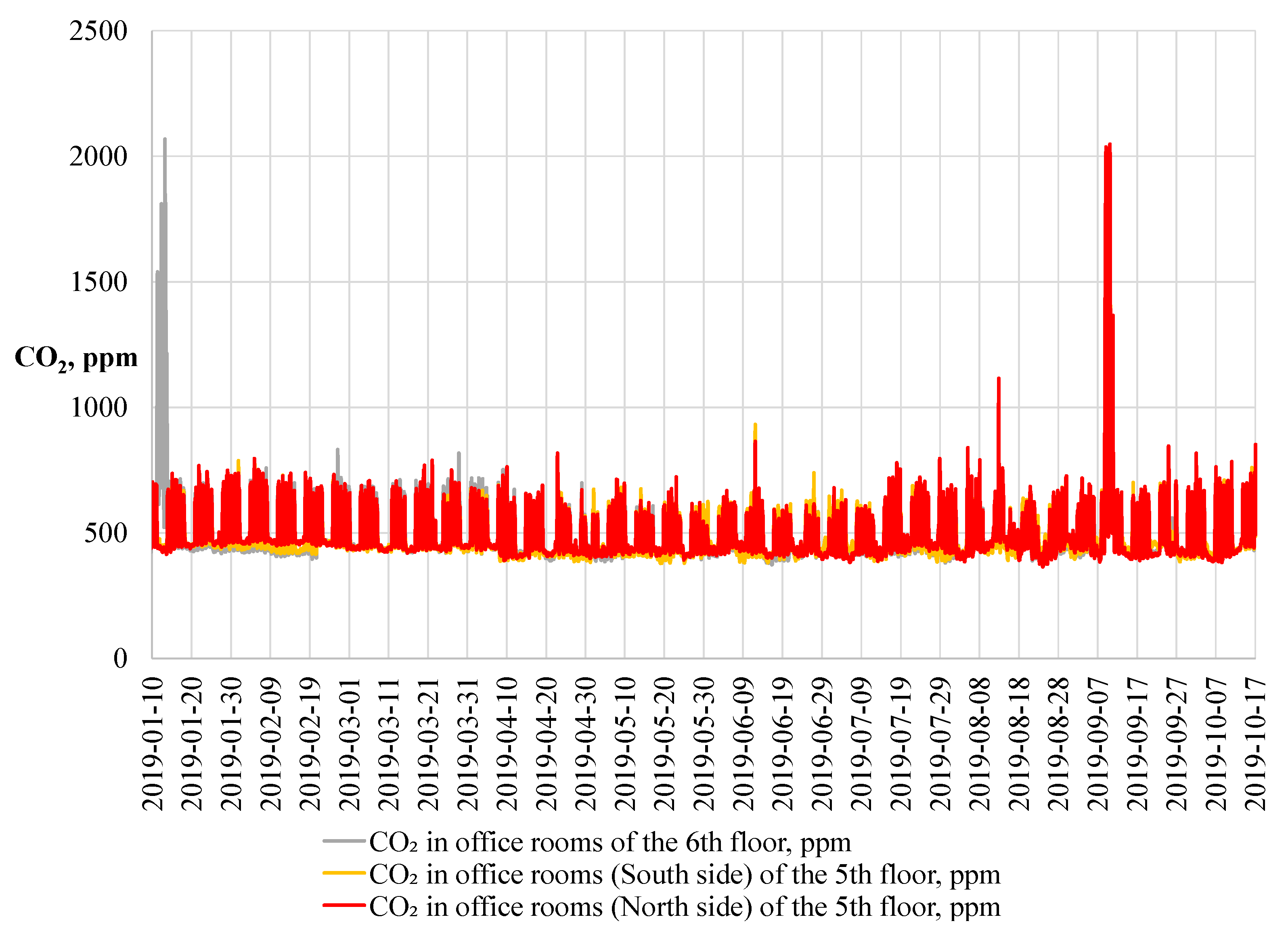
• “Comfort”, which is set automatically during the operating period from 06:00 to 18:00. During operation, ventilation systems operate at 100% efficiency. Supplied air temperature in winter and summer is 22 °C. The concentration of CO₂ in the rooms must not exceed 900 ppm.
• “Economy” is automatically set during non-working and night hours from 18:00 to 06:00 and on weekends. During non-working hours, ventilation systems operate at 30–50% efficiency. The supplied air temperature is 22 °C in winter and 20 °C in summer. The concentration of CO₂ in the rooms must not exceed 1500 ppm.

The BMS controls the fan performance according to the set operating modes of ventilation systems, monitors/records pressure losses in the supply and exhaust ducts every 1 min, and the concentration of CO₂ every 10 min.

The third ventilation system, which serves the rooms of the 5th and 6th floors, has an integrated electrical steam humidifier, which is not available on other floors. Therefore, the BMS monitors/records the relative humidity of the air supplied to these rooms every 3 min. The set value of the relative humidity of the air supplied to the working rooms during the comfort and economy mode is at least 45%.

2.3. Insights of the Functionality of Existing BMS

The installed BMS was analyzed. It was determined that the installed BMS does not collect the data required for the research (indoor climate parameters, HVAC system performance characteristics: efficiency, thermal parameters, etc.). BMS provides the facility manager with only instantaneous characteristics of HVAC systems and indoor air condition parameters. Based on the real-time data, the facility manager can only change the algorithm of the system operation in real-time, identify faults, or adjust the indoor climate. However, the manager cannot determine whether HVAC, lighting, and other systems are operating efficiently, what energy efficiency and comfort would be achieved if minor adjustments were made to the control algorithms introduced, and so on.

The study found that BMS is not an open-source building management system. Each mechanical ventilation system and VRV cooling system has its separate factory automation. As a result, malfunctions and management incompatibilities have been observed with these systems. Thus, in the absence of the possibility of obtaining the required data for the selected period (monthly, quarterly, annual), the actual measurement of indoor climate parameters was performed. However, we are pleased that the building was equipped with a BMS permit to set the control algorithm for HVAC systems and provided energy consumption during the reporting period. The BMS helped to perform the validity of the dynamic energy model qualitatively. It can be argued that the quality level of BMS directly determines the quality of energy model validation.

In order to improve the existing BMS and achieve higher energy efficiency of the existing building, a more advanced energy management strategy is needed. The correct and reasonable data have to be collected and analyzed automatically. The building energy management system (BEMS) or IoT-based strategy could be the right solution for the better energy management of the existing office building.

2.4. Measurement of Indoor Climate Parameters

The building was equipped with an additional measurement system for measuring indoor climate and air parameters in ventilation equipment during the research. The existing BMS does not collect this data. The following main measurements were performed: indoor air temperature, relative humidity, and air quality according to CO₂ concentration. Based on these measurements, the dynamic energy model created in DesignBuilder is calibrated.

Six measuring devices of HOBO (Onset, Falmouth, MA, USA) MX1102 Logger were used to measure indoor climate parameters in office rooms. The device records the temperature from −20 °C to 70 °C, relative humidity—5 ÷ 95%. Temperature measurement accuracy is ±0.35 °C (0 to 50 °C), relative humidity ±2.5% (0 to 90%). These measuring devices are located 1–3 m from the workplaces. The positioning height is ~1.50 ± 0.20 m.

The air supply, extract, exhaust, and intake air temperatures were measured using HOBO U12-008 data loggers adapted for the external measurements by Onset Computer Corporation. The view of the measurements in the ventilation equipment is shown in Figure 2. The temperature measuring sensors TMC20-HD are connected to the HOBO U12-008. The measuring range of the sensor is from −40 °C to 100 °C (when the sensor does not come into contact with water), and the measurement error is ±0.25 °C at measuring temperatures 0 ÷ 50 °C.

The outdoor air temperature, relative humidity, and solar radiation measurements were performed with a data logger HOBO H21-002 adapted for external measurements by the Onset Computer Corporation. The device was placed on the roof and protected from direct sunlight. The data logger can record (and store) various parameters (wind speed and direction, air temperature, etc.) depending on which measuring sensors are connected. A 12-bit temperature and relative humidity sensor S-THB-M008 is connected to the HOBO H21-002 data logger. Sensor temperature measurement ranges from −40 °C to 75 °C, and relative humidity—0 ÷ 100%. Temperature measurement accuracy ±0.21 °C (0 to 50 °C), relative humidity ±2.5% (10 to 90%). The Onset Computer Corporation’s S-LIB-M003 pyrometer is used to measure solar radiation and is connected to a HOBO H21-002 data logger. The measuring range of the pyrometer is from 0 to 1280 W/m², the wavelengths of the measured spectrum range from 300 to 1100 nm. The operating range is –40 °C to 75 °C, and the measurement accuracy is ±10 W/m².

Measurements of the rooms’ indoor climate parameters (air temperature, relative humidity, and CO₂ concentration) lasted from 1 October 2019 to 30 November 2019. The supplied, extracted, exhausted, and intake air parameters (air temperature, relative humidity and CO₂ concentration) were measured in parallel in the building’s three ventilation units (PI-1, PI-2, PI-3). Measurements were performed at one and 5-min intervals, and results are presented as 1-h averages. A calibrated digital energy model based on these measurements was created in DesignBuilder.

3. A Numerical Building ENERGY Model and Calibration Algorithm

The energy model of the office is created using the DesignBuilder program. It is a user-friendly dynamic energy modelling program for the entire building, which allows one to analyze the building energy performance and optimize the alternative solutions applied to it. The following main functions of DesignBuilder were used in the research: detailed simulation of the operation of HVAC systems, thermal comfort, simulation of annual energy demand for heating, cooling, ventilation, and lighting. It should be noted that the program can be compatible with other BIM models.

An initial input data collected from the design documentation, HVAC system control modes, and setpoint parameters of indoor climate programmed in the BMS were used to create the building energy model. The main parameters and their sources are summarised in

Table 4. Main input data used for building energy model.

System or Group	Parameter	Origin
Weather data	Outdoor temperature	Measured on-site
	Relative air humidity	Measured on-site
	Solar radiation	Measured on-site
Heating and Cooling	Heating temperature setpoint	Design and BMS data
	Cooling temperature setpoint	Design and BMS data
	Heating system type/operation mode	Design and BMS data
	Cooling system type/operation mode	Design and BMS data
	The energy efficiency of cooling systems	Design data
Mechanical ventilation	Airflow rate	Design and BMS data
	Heat recovery efficiency	Design and BMS data
	Operation modes	BMS data
	Supplied air temperature in winter	Design and BMS data
	Supplied air temperature in summer	Design and BMS data
Natural ventilation	Window opening status	BMS data
Infiltration	Infiltration air flow rate	Blower door test on-site
Blinds and shading	Technical characteristics (type, colour, automatic control)	Observed on-site
Occupancy	Number of people	Observed on-site
	Density schedule	Default in DesignBuilder
	Working hours	Observed on-site
Lighting	Illumination	Design and BMS data
	Lighting fixtures	Design and BMS data
Heat gains	Occupancy	Design data
	Electrical appliances	Design data
	Lighting	Design data

.

In energy simulation, the operating time of electrical appliances and lighting systems coincides with the time of presence of occupancy. The LED lighting system is controlled by natural lighting, maintaining indoor lighting setpoint during working hours. HVAC systems are grouped according to the designed and installed ventilation systems of the building. The detailed HVAC model consists of: (1) three building zones (ground-3rd floors to the south; ground-3rd floors to the north; 4th–5th floors); (2) the heating substation for heating, ventilation and hot water preparation; (3) heating system with radiators in all building rooms, except WC, shower, changing rooms (near showers), gym with underfloor heating; (4) ventilation systems (AHU-01, AHU-02, AHU-03) with rotary heat exchangers and outdoor cooling units of VRV type (OCU-AHU-01, OCU-AHU-02, OCU-AHU-03); (5) Cooling system—VRV type with HP system for heating and cooling the rooms (VRV-01, VRV-02, VRV-03). A detailed HVAC model created in DesignBuilder is presented in Figure 3.

In the study, the dynamic energy model of the building is calibrated using the methodology typical for empirical validation and using the actual normalized energy consumption of the building and measurement data. Actual and measurement data are compared with the results of the dynamic energy model. The algorithm of building energy model calibration is presented in Figure 4, in which six steps can be distinguished.

Step 1. Development of the initial energy model of the research building:

• Design documentation and theoretical data are used to create the energy model: building architecture, density schedule of occupancy, internal heat gains, lighting data, thermal comfort parameters, technical data of the HVAC system.
• The results of the primary energy model are obtained, inclduing heat demand for heating/ventilation, cooling demand for cooling/ventilation, electricity demand for fans and circulation pumps of technical systems, electricity demand for electrical equipment, and lighting.

Step 2. Acquisition and processing of actual energy consumption data from BMS:

• Data extraction from building heat and electricity meters, identification of HVAC system operating modes, thermal comfort, and air quality settings from BMS are identified.
• Data analysis and processing. The analyzed actual data include heat consumption for heating/ventilation, electricity consumption for heating/cooling, fans of ventilation systems and circulation pumps, lighting and electrical equipment, and other electricity consumers (elevators, outdoor lighting, etc.). Actual heat consumption and heat demand for heating determined by the energy simulation model are normalized by degree-days of reference year [53].

Step 3. Performing measurements:

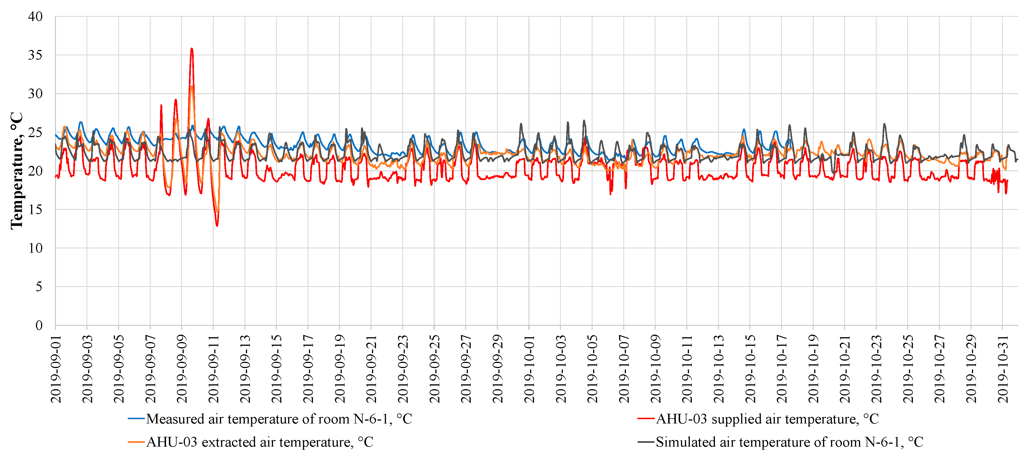
• Data of indoor climate parameters (air temperature, relative humidity) and air quality measurements of selected rooms in the building, air temperature data, relative humidity and CO₂ concentration in the extraction line in ventilation systems are measured. As an example, one of the measurement points is shown, which is shown in the energy model fragment—room N-6-1 (Figure 5), where the location of the measuring device HOBO MX1102 Logger SN20468904 of indoor climate parameters is shown together.
• Processing and interpretation of the obtained results of measurements are made.

Step 4. Model calibration is carried out to achieve the reliability of the obtained results of the primary (basic) model and the compatibility of the numerical energy model and the BMS. Actual and measured data are compared with the results of the theoretical dynamic energy model.

Step 5. Model calibration by modifying parameters. The following parameters were examined and adjusted to achieve a higher coincidence between the results of the energy model and the measurements:

• Occupancy intensity indicator (from 10 m²/occupant changed to 20 m²/occupant);
• Installed electrical power of electrical office equipment (from 10,764 W/m² changed to 5 W/m²);
• Lighting intensity (from 8.51 W/m² changed to 5 W/m²);
• The actual setpoint of room air temperature in the winter and summertime, according to the BMS;
• Operating modes/schedules and control for HVAC systems set in BMS.

Step 6. The compatibility of the energy model and the BMS is presented, where the obtained energy model corresponds to the experimental data. The results of the dynamic energy model are analyzed.

4. Results and Discussion

4.1. The Results of the Measurement: Analysis of Separate Parameters

The paper presents the measurements of the 5th and 6th floors of the building and the AHU-03 ventilation unit. The general variation of the indoor climate parameters for the measured period (almost ten months) is presented in Figure 6, Figure 7 and Figure 8. The measurement time step is 5 min. The graphs show average hourly values. Figure 6 shows the results of measurements of air temperatures in the working area of the 5th and 6th floors and the AHU-03 ventilation unit.

According to the outdoor air temperature, the cold, intermediate, and warm periods are identified. As can be seen, they are characterized by differences between indoor and outdoor temperatures. The measurement data found that the supply air temperature was controlled until the 27 March 2019 (i.e., heating is underway). The supplied air heating started due to the significant air temperature fluctuation from the 15 September to the 16th. During the day, the temperature was raised, and at night it was lowered. On weekends it remained constant. From this time on, it considered that heating season started.

During the heating season, the indoor air temperature deviated slightly from the normative values. The indoor air temperature was maintained from 22 °C to 24 °C in the cold period and from 23 °C to 25 °C during the warm period. Therefore, it indicates that the heating system of the building is managed reliably.

During the warm period, the same tendency is observed when the room’s air temperature deviates from the standard values insignificantly but does not exceed the values of the sufficient thermal environment.

Figure 7 shows the relative humidity of the rooms (zones) on the 5th and 6th floors, served by the AHU-03 air handling unit.

It can be seen that relative humidity was maintained in the rooms during the cold period. On a dark background, normative relative humidity values from 40% to 60% are given. On a light grey background (including the dark grey area), the relative humidity values of the indoor air, which may not exceed 75%, is given. The relative humidity of the extract air from the premises during the cold period (see the area bounded by the black line in Figure 7) fluctuated within the limits of the normative values, and short-term deviations below the limits of 40% are rare. During the warm period (see Figure 7), the air humidification in the ventilation unit is switched off, and it can be observed that the relative humidity often falls or exceeds the standard values but does not exceed a sufficient relative humidity value (75%).

Figure 7 shows that the relative humidity in the measured 5 and 6 high zones (see the red, yellow and grey lines) often falls below the normal value, although the extract air rarely drops below 40% during the cold period. This trend is visible since the relative humidity of indoor air of the rooms served by the AHU-03 is controlled by the relative humidity of the extracted air and not by the relative humidity of the indoor air of separate rooms. During the warm period, the relative humidity often exceeds the normative values. This issue is due to the high relative humidity values of supplied air (Figure 7, blue line), which is not controlled during intermediate and warm periods. Therefore, this situation shows that the office rooms should be dehumidified during the warm period to achieve a high level of thermal comfort.

Figure 8 shows the CO₂ measurements in the room of the 5th and 6th floors and the AHU-03 ventilation unit. It can be seen that the CO₂ concentration in the room exceeded 1000 ppm only several times during the whole measurement period. This increase in CO₂ concentration was due to the ventilation system being switched off or the indoor measuring device being placed too close to a working person, which could affect the results.

The average CO₂ value for the whole measurement period was about 488 ppm, and the average operating hours ranged from 600 to 800 ppm. This data shows that the office rooms have the highest air quality, corresponding to the indoor air category of IDA-1 (up to 800 ppm). At the same time, it shows how to save energy costs (electricity and heat) during the operation of the premises by reducing air quality to the category of IDA-2, which corresponds to the design category applicable to this building.

4.2. Assessment of the Whole Measurement Period

Based on the actual measurements, the conditions of the indoor climate maintained in the office rooms were determined, and a summary of the results of the measurement data analysis was created (see

Table 5. Summary of results of indoor climate parameters measurement data.

Season	Troom, average, °C/RHroom, average, % 1		Tsupply, AHU-01, °C 2		Tsupply, AHU-02, °C 3		Tsupply, AHU-03, °C/RHsupply, AHU-03, % 4
	WKH	nWKH	WKH	nWKH	WKH	nWKH	WKH	nWKH
Cold (winter)	23 °C/5-6 a.: RH 42 ÷ 46.5%	21 °C/NA	23.5/NA	19/NA	22/NA	20/NA	22 °C/RH 45.5 ÷ 48.5%	18 °C/NA
Intermediate 1 (spring)	22.5 °C/5-6 a.: RH 43.8 ÷ 47.3%	24 °C/NA	20/NA	22/NA	20/NA	22/NA	20.5 °C/RH 44 ÷ 52%	23 °C/NA
Warm (summer)	24 °C/NA	25 °C/NA	20/NA	23/NA	19.5/NA	21/NA	19.7 °C/NA	24 °C/NA
Intermediate 2 (Autumn)	22 °C/5-6 a.: RH 42.6 ÷ 44.7%	24 °C/NA	22/NA	20/NA	22/NA	20/NA	20 °C/RH 44 ÷ 48%	22 °C/NA

¹—statistically most frequently iterative average air temperature (T_{room, average}, °C) and relative humidity (RH_{room, average},%) of heated/cooled rooms; ²—statistically most frequently iterative supply air temperature of AHU-01 system (T_{supply, AHU-01}, °C); ³—statistically most frequently iterative supply air temperature of AHU-02 system (T_{supply, AHU-02}, °C); ⁴—statistically most frequently iterative supply air temperature of AHU-03 system (T_{supply, AHU-03}, °C) and relative humidity (RH_{supply, AHU-03},%); WKH/nWKH—working hours/non-working hours; NA—indoor climate parameters are not ensured.

). The actual values of the thermal comfort parameters obtained by statistical processing of the measurement data are presented by compiling a histogram for each period, adapted to show the distribution of quantitative statistical data (in this case, measured indoor air temperatures). Table 5 shows only the most frequently repeated values in the interval statistical cell used later in the DesignBuilder model.

Based on the experimental data, it can be seen that the operating modes of HVAC systems and the maintained indoor climate parameters in the rooms change during the year. Therefore four seasons/periods were distinguished:

• Cold period (winter), when the outdoor temperature is below 0° C (T_outside < −5 °C), in the case study, this period covered from the 1 November to the 28 February;
• The 1st intermediate period (spring), when the outdoor temperature ranges from −5 °C to +16 °C (−5 °C < T_outside < 16 °C), the duration is from the 1 March to the 30 April;
• Warm period (summer), when the outdoor air temperature is above +16 °C (T_outside > +16 °C), its duration is from 1 June to the 31 August;
• The 2nd intermediate period (autumn), when the outdoor air temperature ranges from −5 °C to +16 °C (−5 °C < T_outside < 16 °C), the duration is from the 1 September to the 31 October.

Identified periods allowed a better understanding of the operation of the building as a whole and its systems.

4.3. Model Calibration and Numerical Results

The measurement results of indoor climate parameters and the actual operation of the AHU-03 ventilation system presented above are considered to compare the simulated and measured results. The comparison includes the supplied/extracted air parameters of the AHU-03 system and the indoor climate N-6-1 room on the sixth storey (see Figure 5) in different seasons. During the measurements, it was observed that the indoor climate parameters (the required air temperature and relative humidity) of the rooms at the 5th and 6th floors are more constant, less variable during the day and month compared to the 1st, 2nd, 3rd, and 4th floors served by AHU-01 and AHU-02 ventilation systems. AHU-01 and AHU-02 are without air humidification. The results show that the control of the AHU-03 system is better and more reliable.

Figure 9 shows the measured and simulated air temperature values of the N-6-1 room on the sixth floor during the winter season, the measured values of the supplied, and exhausted air temperature of the AHU-03 ventilation system. A comparison of the simulated data of other seasons with the measurement data is provided in Appendix A.

The graph shows that the temperature modes maintained in the rooms, based on the actual measurements and the simulated data, partially overlap. The most common temperature difference is obtained from 0.5 to 1.0 °C. Visible discrepancies are due to external errors, differences between climatic data (actual and IWEC data formats), and differences due to users’ behaviour and the impact of the building itself. The general trend (Figure 9 and Appendix A) shows that, based on BMS monitoring, differences between actual schedules (e.g., occupancy schedule), and HVAC systems control strategies have been successfully minimized.

After analyzing the simulated results for the whole year, it was identified that the following indicators cover the annual heat/cool balance of the building:

• Cooling demand for room cooling and ventilation—180 MWh/year;
• Heat demand for ventilation air heaters—50 MWh/year;
• Heat demand for space heating with VRV system—410 MWh/year;
• Heat demand for space heating with a radiator heating system—90 MWh/year.

Additional numerical values obtained during the dynamic energy simulation are presented in Figure 10.

The study of the annual balance showed that the highest needs are the heat demand from central district heating (heating (other fuels)) is 26.56 kWh/m²·a and the electricity demand for air humidification (auxiliary energy) is 22.25 kWh/m²·a. In addition, the building still needs electricity for space heating (VRF system) is 17.26 kWh/m²·a (heating (electricity)) and 7.41 kWh/m²·a for space cooling (cooling (electricity)). Therefore, the next step to improve the existing office energy performance is to focus on energy-efficient measures to reduce the heat demand for space heating and electricity demand for air humidification. Figure 10 shows that the most significant energy-saving potential is energy-efficient office equipment, lighting system and efficient ventilation systems, and the selection of optimal operating strategies for HVAC systems.

The simulated data of annual building energy balance were compared with the actual energy consumption in 2019 obtained from the heat/cooling/electricity meters installed in the building. The comparative analysis is presented in

Table 6. Comparison of actual and simulated building energy balances.

Energy, Units	Source	Consumer/System	Normalized Actual Data (2019)	Normalized Energy Model Data
Heat, MWh/year	District Heating networks	Heating system (radiators)	96.60	–
		Ventilation system (water-based heating coils)	5.41	–
		Total, MWh/year (kWh/m2·a)	102.2 (18.50)	95.41 (17.28)
Electricity, MWh/year	Electrical networks	Space heating with VRV systems	96.62	95.31
		AHU reversible heating/cooling coil (VRV type) for air heating	23.8	17.84
		VRV cooling system	21.7	40.93
		AHU reversible heating/cooling coil (VRV type) for air cooling	17.7
		AHU fans	139.14	115.61
		The electric steam generator of AHU-03 for air humidification 1	78.98	122.91
		Lighting and electrical appliances of office rooms	152.98	159.17
		Lighting and electrical appliances of restaurant	18.38
		Lighting and electrical appliances of sports club	2.14
		Total, MWh/year (kWh/m2·a)	551.45 (99.85)	551.77 (99.91)

¹—There is no separate electricity meter of air humidification installed in the building. The electric steam generator is connected to a common input meter, so all electricity consumers in the building were deducted from the total consumption. In this way, the actual electricity demand for air humidification was determined.

.

Table 6 shows that the results of the model calibration process allowed us to evaluate the reliability of the developed building energy model and determine the size of the errors. The data of the calibrated model and the actual energy meters in 2019 differ:

• 6.5%, when estimating the total heat demand of the building;
• 0.06%, when estimating the total electricity demand of the building.

4.4. Limitations of the Study

The case study building has been awarded the BREEAM New Construction “very good” level building sustainability certificate. According to the “As-built stage report of an evaluation of energy efficiency for BREEAM International New Construction”, the heat demand from central district heating is 9.36 kWh/m²·a, electricity for space heating 6.92 kWh/m²·a (VRF system), 2.69 kWh/m²·a for space cooling, and 5.35 kWh/m²·a for indoor air humidification of the 5th and 6th floors. The results of the “As-built stage report” and the actual BMS data show that the design assumptions for the operation/management of the HVAC systems are very different from the actual energy consumption of the building. The actual energy consumption of the building is significantly higher (the actual energy consumption for space heating and cooling alone is 2.7 times higher). Therefore, the building manager/supervisor has to focus on the potential energy savings.

The analysis of performed measurements shows that space heating is the most significant energy user due to too high indoor air temperature maintained during the winter (from 23 °C to 24 °C). The results of the calibrated energy model show that a significant amount of energy is recovered in the heat exchangers of ventilation units since the temperature of the extracted air is higher than 22 °C even during the cold period. By controlling the supplied air temperature according to the extracted air temperature, it would be possible to supply air to the office rooms at a lower temperature (within the permissible limits), thus ensuring efficient assimilation of excess heat and energy savings.

Significant electricity demand consists of ventilation system fans, lighting systems, electric steam generator for air humidification, and VRV system (operating in heating mode). The specific fan power (SFP) of ventilation systems accepted during the simulation was 0.48 Wh/m³, which did not exceed the recommended value of 0.55 Wh/m³. Thus, the potential for energy savings could be provided by more efficient strategies used for operating ventilation systems, leading to more efficient control of these systems. The energy savings potential is energy-efficient lighting systems, ventilation systems, air humidification systems, and the prediction of their operating strategies.

Despite the contributions of the present study, and the identification of main issues due to the energy savings, this study has limitations. First, the current research does not include the most reasonable energy savings measures that increase the energy performance of the existing office. Second, the authors of this case study do not present the recommendations or technical specifications for more efficient building maintenance, providing primary level indications to the supervisor and owner/manager. Therefore, the scope of the future study will be to present the algorithm of an expert system of sustainable building energy performance at the operation and maintenance stage, which enables a selection of the most suitable energy savings measures according to an indicator of sustainable development.

5. Conclusions

In order to develop the energy model of the building and achieve the highest possible reliability of its results, measurements of the indoor climate parameters were performed, and the building management system and the data obtained by it were analyzed. The analysis of the office rooms measured and real-time indoor climate parameters showed that the design assumptions made for the operation and management of HVAC systems differ significantly from the actual energy consumption. It showed that the design assumptions have a high impact on the accuracy of the building dynamic energy model. In addition, the measurements showed that the air temperature and CO₂ concentration in the office rooms served by the ventilation equipment meet the normative values, and the relative humidity satisfies only the values of a good thermal environment. It was found that the category of CO₂ concentration most often maintained in the office rooms corresponds to IDA 1 (very good air quality), which can be reduced to IDA category 2 in terms of saving energy.

The building dynamic energy model calibration was performed based on the actual building energy consumption analysis and measurements of the indoor climate parameters from 1 November 2019 to 30 November 2019. Based on the available data, the calibrated model results showed that the BMS installed in the building allowed us to establish control algorithms for HVAC systems and provided valuable information on energy consumption. It indicates that the level of BMS directly determines the quality of the digital model calibration. A total discrepancy of 6.5% was found in the case study by comparing the building’s actual and simulated heat demand.

The developed building energy model can be applied to the continuous improvement of energy performance by implementing the principles of energy demand management and evaluating possible modernization measures. In future, it is crucial to examine the impact of the chosen solutions based on this model to achieve higher/better energy efficiency and sustainability criteria.

References

1. European Commission. Comprehensive Study of Building Energy Renovation Activities and the Uptake of Nearly Zero-Energy Buildings in the EU FINAL Report; European Commission: Brussels, Belgium, 2019. [Google Scholar]
2. EASAC. Decarbonization of Buildings: For Climate, Health and Jobs; Policy Report 43; EASAC: Halle, Germany, 2021; ISBN 9783804732391. [Google Scholar]
3. Džiugaitė-Tumėnienė, R.; Motuzienė, V.; Šiupšinskas, G.; Čiuprinskas, K.; Rogoža, A. Integrated assessment of energy supply system of an energy-efficient house. Energy Build. 2017, 138, 443–454. [Google Scholar] [CrossRef]
4. Santos-Herrero, J.M.; Lopez-Guede, J.M.; Flores-Abascal, I. Modeling, simulation and control tools for nZEB: A state-of-the-art review. Renew. Sustain. Energy Rev. 2021, 142, 110851. [Google Scholar] [CrossRef]
5. Vujnović, N.; Dović, D. Cost-optimal energy performance calculations of a new nZEB hotel building using dynamic simulations and optimization algorithms. J. Build. Eng. 2021, 39. [Google Scholar] [CrossRef]
6. Aste, N.; Adhikari, R.S.; Buzzetti, M.; Del Pero, C.; Huerto-Cardenas, H.E.; Leonforte, F.; Miglioli, A. nZEB: Bridging the gap between design forecast and actual performance data. Energy Built Environ. 2020. [Google Scholar] [CrossRef]
7. Cunha, F.O.; Oliveira, A.C. Benchmarking for realistic nZEB hotel buildings. J. Build. Eng. 2020, 30, 101298. [Google Scholar] [CrossRef]
8. Magni, M.; Ochs, F.; de Vries, S.; Maccarini, A.; Sigg, F. Detailed cross comparison of building energy simulation tools results using a reference office building as a case study. Energy Build. 2021, 250. [Google Scholar] [CrossRef]
9. Abi Shdid, C.; Younes, C. Validating a new model for rapid multi-dimensional combined heat and air infiltration building energy simulation. Energy Build. 2015, 87, 185–198. [Google Scholar] [CrossRef]
10. Wang, R.; Lu, S.; Feng, W. A novel improved model for building energy consumption prediction based on model integration. Appl. Energy 2020, 262, 114561. [Google Scholar] [CrossRef]
11. Mikučioniene, R.; Martinaitis, V.; Keras, E. Evaluation of energy efficiency measures sustainability by decision tree method. Energy Build. 2014, 76, 64–71. [Google Scholar] [CrossRef]
12. Neymark, J.; Judkoff, R.; Knabe, G.; Le, H.T.; Dürig, M.; Glass, A.; Zweifel, G. Applying the building energy simulation test (BESTEST) diagnostic method to verification of space conditioning equipment models used in whole-building energy simulation programs. Energy Build. 2002, 34, 917–931. [Google Scholar] [CrossRef]
13. Guyot, D.; Giraud, F.; Simon, F.; Corgier, D.; Marvillet, C.; Tremeac, B. Building energy model calibration: A detailed case study using sub-hourly measured data. Energy Build. 2020, 223, 110189. [Google Scholar] [CrossRef]
14. Benzaama, M.H.; Rajaoarisoa, L.H.; Ajib, B.; Lecoeuche, S. A data-driven methodology to predict thermal behavior of residential buildings using piecewise linear models. J. Build. Eng. 2020, 32. [Google Scholar] [CrossRef]
15. Harish, V.S.K.V.; Kumar, A. A review on modeling and simulation of building energy systems. Renew. Sustain. Energy Rev. 2016, 56, 1272–1292. [Google Scholar] [CrossRef]
16. Afroz, Z.; Shafiullah, G.M.; Urmee, T.; Higgins, G. Modeling techniques used in building HVAC control systems: A review. Renew. Sustain. Energy Rev. 2018, 83, 64–84. [Google Scholar] [CrossRef]
17. Zhang, D.; Xia, X.; Cai, N. A dynamic simplified model of radiant ceiling cooling integrated with underfloor ventilation system. Appl. Therm. Eng. 2016, 106, 415–422. [Google Scholar] [CrossRef]
18. Chintala, R.H.; Rasmussen, B.P. Automated multi-zone linear parametric black box modeling approach for building HVAC systems. In Proceedings of the ASME 2015 Dynamic Systems and Control Conference, DSCC 2015, Columbus, OH, USA, 28–30 October 2015; p. 10. [Google Scholar]
19. Thomas, B.; Soleimani-Mohseni, M. Artificial neural network models for indoor temperature prediction: Investigations in two buildings. Neural Comput. Appl. 2007, 16, 81–89. [Google Scholar] [CrossRef]
20. Afram, A.; Fung, A.S.; Janabi-Sharifi, F.; Raahemifar, K. Development and performance comparison of low-order black-box models for a residential HVAC system. J. Build. Eng. 2018, 15, 137–155. [Google Scholar] [CrossRef]
21. Mazuroski, W.; Berger, J.; Oliveira, R.C.L.F.; Mendes, N. An artificial intelligence-based method to efficiently bring CFD to building simulation. J. Build. Perform. Simul. 2018, 11, 588–603. [Google Scholar] [CrossRef]
22. Attoue, N.; Shahrour, I.; Younes, R. Smart building: Use of the artificial neural network approach for indoor temperature forecasting. Energies 2018, 11, 395. [Google Scholar] [CrossRef] [Green Version]
23. Wang, J.; Li, S.; Chen, H.; Yuan, Y.; Huang, Y. Data-driven model predictive control for building climate control: Three case studies on different buildings. Build. Environ. 2019, 160. [Google Scholar] [CrossRef]
24. Qiu, S.; Li, Z.; Pang, Z.; Zhang, W.; Li, Z. A quick auto-calibration approach based on normative energy models. Energy Build. 2018, 172, 35–46. [Google Scholar] [CrossRef]
25. Coakley, D.; Raftery, P.; Keane, M. A review of methods to match building energy simulation models to measured data. Renew. Sustain. Energy Rev. 2014, 37, 123–141. [Google Scholar] [CrossRef] [Green Version]
26. Kim, Y.K.; Bande, L.; Aoul, K.A.T.; Altan, H. Dynamic energy performance gap analysis of a university building: Case studies at UAE university campus, UAE. Sustainability 2021, 13, 120. [Google Scholar] [CrossRef]
27. Bielskus, J.; Motuzienė, V.; Vilutiene, T.; Indriulionis, A. Occupancy Prediction Using Differential Evolution Online Sequential Extreme Learning Machine Model. Energies 2020, 13, 4033. [Google Scholar] [CrossRef]
28. Cuerda, E.; Guerra-Santin, O.; Sendra, J.J.; Neila, F.J. Understanding the performance gap in energy retrofitting: Measured input data for adjusting building simulation models. Energy Build. 2020, 209, 109688. [Google Scholar] [CrossRef]
29. Dartevelle, O.; van Moeseke, G.; Mlecnik, E.; Altomonte, S. Long-term evaluation of residential summer thermal comfort: Measured vs. perceived thermal conditions in nZEB houses in Wallonia. Build. Environ. 2021, 190, 107531. [Google Scholar] [CrossRef]
30. Bhandari, M.; Shrestha, S.; New, J. Evaluation of weather datasets for building energy simulation. Energy Build. 2012, 49, 109–118. [Google Scholar] [CrossRef]
31. Ruiz, G.R.; Bandera, C.F. Validation of calibrated energy models: Common errors. Energies 2017, 10, 1587. [Google Scholar] [CrossRef] [Green Version]
32. Marshall, A.; Fitton, R.; Swan, W.; Farmer, D.; Johnston, D.; Benjaber, M.; Ji, Y. Domestic building fabric performance: Closing the gap between the in situ measured and modelled performance. Energy Build. 2017, 150, 307–317. [Google Scholar] [CrossRef]
33. Zheng, O.; Eisenhower, B. Leveraging the analysis of parametric uncertainty for building energy model calibration. Build. Simul. 2013, 6, 365–377. [Google Scholar] [CrossRef]
34. Fathalian, A.; Kargarsharifabad, H. Actual validation of energy simulation and investigation of energy management strategies (Case Study: An office building in Semnan, Iran). Case Stud. Therm. Eng. 2018, 12, 510–516. [Google Scholar] [CrossRef]
35. Cacabelos, A.; Eguía, P.; Míguez, J.L.; Granada, E.; Arce, M.E. Calibrated simulation of a public library HVAC system with a ground-source heat pump and a radiant floor using TRNSYS and GenOpt. Energy Build. 2015, 108, 114–126. [Google Scholar] [CrossRef]
36. Li, W.; Tian, Z.; Lu, Y.; Fu, F. Stepwise calibration for residential building thermal performance model using hourly heat consumption data. Energy Build. 2018, 181, 10–25. [Google Scholar] [CrossRef]
37. Ahmed, T.M.F.; Rajagopalan, P.; Fuller, R. Experimental validation of an energy model of a day surgery/procedure centre in Victoria. J. Build. Eng. 2017, 10, 1–12. [Google Scholar] [CrossRef]
38. Zou, P.X.W.; Alam, M. Closing the building energy performance gap through component level analysis and stakeholder collaborations. Energy Build. 2020, 224, 110276. [Google Scholar] [CrossRef]
39. Pappalardo, M.; Reverdy, T. Explaining the performance gap in a French energy efficient building: Persistent misalignment between building design, space occupancy and operation practices. Energy Res. Soc. Sci. 2020, 70, 101809. [Google Scholar] [CrossRef]
40. Heo, Y.; Choudhary, R.; Augenbroe, G.A. Calibration of building energy models for retrofit analysis under uncertainty. Energy Build. 2012, 47, 550–560. [Google Scholar] [CrossRef]
41. Lim, H.; Zhai, Z.J. Influences of energy data on Bayesian calibration of building energy model. Appl. Energy 2018, 231, 686–698. [Google Scholar] [CrossRef]
42. Asadi, S.; Mostavi, E.; Boussaa, D.; Indaganti, M. Building energy model calibration using automated optimization-based algorithm. Energy Build. 2019, 198, 106–114. [Google Scholar] [CrossRef]
43. Ascione, F.; Bianco, N.; Iovane, T.; Mastellone, M.; Maria, G. Is it fundamental to model the inter-building effect for reliable building energy simulations? Interaction with shading systems. Build. Environ. 2020, 183, 107161. [Google Scholar] [CrossRef]
44. Figueiredo, A.; Kämpf, J.; Vicente, R.; Oliveira, R.; Silva, T. Comparison between monitored and simulated data using evolutionary algorithms: Reducing the performance gap in dynamic building simulation. J. Build. Eng. 2018, 17, 96–106. [Google Scholar] [CrossRef]
45. Iddianozie, C.; Palmes, P. Towards smart sustainable cities: Addressing semantic heterogeneity in Building Management Systems using discriminative models. Sustain. Cities Soc. 2020, 62, 102367. [Google Scholar] [CrossRef]
46. GhaffarianHoseini, A.; Zhang, T.; Nwadigo, O.; GhaffarianHoseini, A.; Naismith, N.; Tookey, J.; Raahemifar, K. Application of nD BIM Integrated Knowledge-based Building Management System (BIM-IKBMS) for inspecting post-construction energy efficiency. Renew. Sustain. Energy Rev. 2017, 72, 935–949. [Google Scholar] [CrossRef] [Green Version]
47. Oti, A.H.; Kurul, E.; Cheung, F.; Tah, J.H.M. A framework for the utilization of Building Management System data in building information models for building design and operation. Autom. Constr. 2016, 72, 195–210. [Google Scholar] [CrossRef] [Green Version]
48. Eini, R.; Linkous, L.; Zohrabi, N.; Abdelwahed, S. Smart building management system: Performance specifications and design requirements. J. Build. Eng. 2021, 39, 102222. [Google Scholar] [CrossRef]
49. Borrelli, M.; Merema, B.; Ascione, F.; Francesca De Masi, R.; Peter Vanoli, G.; Breesch, H. Evaluation and optimization of the performance of the heating system in a nZEB educational building by monitoring and simulation. Energy Build. 2021, 231, 110616. [Google Scholar] [CrossRef]
50. Kučera, A.; Pitner, T. Semantic BMS: Allowing usage of building automation data in facility benchmarking. Adv. Eng. Inform. 2018, 35, 69–84. [Google Scholar] [CrossRef]
51. Guerra-Santin, O. Relationship between building technologies, energy performance and occupancy in domestic buildings. Living Labs Des. Assess. Sustain. Living 2016, 333–344. [Google Scholar] [CrossRef]
52. Foucquier, A.; Robert, S.; Suard, F.; Stéphan, L.; Jay, A. State of the art in building modelling and energy performances prediction: A review. Renew. Sustain. Energy Rev. 2013, 23, 272–288. [Google Scholar] [CrossRef] [Green Version]
53. Martinaitis, V.; Rogoža, A.; Šiupšinskas, G. Energijos Vartojimo Pastatuose Auditas; Technika: Vilnius, Lithuania, 2012; ISBN 9786094571800. [Google Scholar]
Figure 1. 3D model of an office building of a case study.
Energies 14 06419 g001
Figure 2. Measuring points inside the AHU: (a) section of supplied air fan; (b) intake air filter; (c) extracted and exhausted air ducts; (d) measuring device on the case of AHU.
Energies 14 06419 g002
Figure 3. A detailed HVAC model of the office.
Energies 14 06419 g003
Figure 4. Calibration algorithm of building energy model.
Energies 14 06419 g004
Figure 5. Room N-6-1 (Zone 11) in the energy model and the location of the measuring device SN: 20,468,904 of indoor climate parameters.
Energies 14 06419 g005
Figure 6. Measured outdoor and indoor air temperatures of rooms serviced by the AHU-03 ventilation system: (a) measured outside air temperature; (b) measured indoor air temperatures.
Energies 14 06419 g006
Figure 7. Measured relative humidity of rooms serviced by the AHU-03 ventilation system: (a) measured outside air relative humidity; (b) measured indoor air relative humidity.
Energies 14 06419 g007
Figure 8. Measured CO2 concentration in the rooms of the 5th and 6th floors.
Energies 14 06419 g008
Figure 9. Measured/simulated N-6-1 room and measured AHU-03 ventilation system supplied/extracted air temperatures in winter.
Energies 14 06419 g009
Figure 10. Annual building energy balance.
Energies 14 06419 g010