The Thermal—Flow Processes and Flow Pattern in a Pulsating Heat Pipe—Numerical Modelling and Experimental Validation

Abstract

The aim of the article is to numerically model a two-dimensional multiphase flow based on the volume of fluid method (VOF) in a pulsating heat pipe (PHP). The current state of knowledge regarding the modeling of these devices was studied and summarised. The proposed model is developed within open source software, OpenFOAM, based on the predefined solver called interPhaseChangeFoam. The analyses were carried out in terms of the influence of four different mass transfer models between the phases, proposed by Tanasawa, Lee, Kafeel and Turan, and Xu et al. on the shape and dynamics of the internal flow structures. The numerical models were validated against data obtained from a specially designed experimental setup, consisting of three bends of pulsating heat pipes. The numerical calculations were carried out with ethanol being treated as a working medium and the initial and boundary conditions taken directly from the measurement procedures. The variable input parameter for the model was the heat flux implemented in the evaporation section and a fixed temperature applied to the condensation section. The flow structures obtained from the numerical analyses were compared and discussed with the flow structures gained from experimental studies by employing a high speed camera. In addition, to verify the quantitative results obtained from the numerical analyses with the experimental data, a technique called particle image velocimetry (PIV) was used for the velocity vector field. For the analysed velocity ranges, the relative error obtained was reached at the level of 10%.

1. Introduction

Nowadays energy-saving trends force the miniaturization of thermal devices and for them to be designed with as high efficiency as possible. To fulfil these demands, thermal devices have to feature the transference of high heat fluxes [1]. One such device is a pulsating heat pipe (PHP) [2,3,4]. It is built from capillary tubes of meandrical shape that are usually closed. Three parts of a PHP can be distinguished, i.e., condenser, evaporator, and adiabatic sections. Due to the phase change phenomenon of a working fluid, a PHP can transfer heat fluxes in the order of several dozen $\mathrm{W}/\left({\mathrm{m}}^2\mathrm{K}\right)$.The additional merits of a PHP are its self-sustaining work and the ability to have small sizes. Therefore, PHPs are being intensively researched to better understand how they work.

Most of the studies concerning PHPs are experimental ones and focused on the visualization of two-phase flow [5,6,7,8,9]. However, to get more insight into the phenomena occurring in a PHP, numerical modelling based on Computational Fluid Dynamics (CFD) is increasingly being used. Wang et al. [10], presented a two-dimensional model of a closed-loop pulsating heat pipe with one loop. Using the Volume Of Fluid (VOF) method, the authors numerically studied the influence of different ratios of the evaporator length to that of the condenser for various input power and filling ratio (FR) on the thermal performance of a PHP. The results were compared with the available data in the literature for similar conditions. Ghanta and Pattamatta [11] elaborated a compressible phase change solver of a part-unit cell of a PHP. The code was implemented in OpenFOAM software. In the model, only evaporation was taken into account. The model was validated against analytical test cases and experiments from the literature. The authors discussed the effect of evaporator length, evaporator superheat, and FR on the performance of the PHP.

Wang et al. [12] numerically and experimentally investigated a single-loop PHP with corrugated walls. The numerical results showed good consistency with those of experiments. The authors changed the input power and the FR of the working fluid. The results revealed that the corrugation configuration is beneficial for heat transfer performance and the thermal resistance decreased almost by $40\%$. Dang et al. [13] numerically studied a rack cooling system with a PHP and an inner duct dedicated for cooling computer processors. The authors proposed a simple model of a PHP based on conduction heat transfer. The numerical results of the processor temperature were compared with the experimental ones, observing similar results. Nonetheless, the flow phenomena inside the PHP were not investigated.

Pouryoussefi and Zhang [14] performed two-dimensional numerical studies of a multiturn closed-loop PHP using the volume of fluid (VOF) method. The results showed the formation of slug and plug regimes in the PHP, however the model was not verified with experimental data. The authors conducted additional studies on chaos and observed chaotic behaviour under various operating conditions. It was noted that this study could be helpful for developing a 3D model of a PHP. Venkata and Bhramara [15] presented a CFD analysis of a PHP filled with binary mixtures and with different internal diameters. The method used was VOF implemented in Ansys CFX software, however the model of mass transfer was not given. The results were compared with experiments from the literature obtaining similar trends of thermal resistance of the PHP. Wang and Bai [16] studied a closed-loop PHP with a partial horizontal structure. The authors used the VOF method implemented in Ansys FLUENT software and verified the model with data from the literature. The PHP was investigated under different filling ratios, heating power, and height differences between the evaporator and condenser sections. It was found that the proposed PHP features the critical vertical start-up height and the thermal resistance decreases when increasing the heights difference between the evaporator and condenser sections.

Li et al. [17] numerically studied the influence of microencapsulated phase change material (MEPCM) on the anti-dry-out capability of a PHP. The model was validated by comparison with the results from the literature. The authors found that the MEPCM can be beneficial for the anti-dry-out capability of a PHP in a certain range of phase change temperatures. Sagar et al. [18] analysed a two-dimensional cryogenic PHP under varying gravity conditions and diverse filling ratios. The VOF method in combination with Lee mass transfer model was used to model phase change phenomena in a PHP. Nonetheless, a validation of the model was not performed. The numerical simulations established that for low gravity conditions the flow patterns are more stable which advantageously affects the heat transfer.

Choi and Zhang [19] used OpenFOAM in-house code to numerically model a two-dimensional PHP with multiple turns. The authors modified the Lee model based on the mass balance between evaporation and condensation. The symmetric and asymmetric configuration of the PHP was investigated, showing that in the lateral case the circulation started earlier. The authors compared the results of the thermal resistance with data from the literature, obtaining very good agreement. The validated model was then applied to conduct a parametric analysis of the PHP where the effect of different geometries and the Bond number was tested.

Barba et al. [20] performed 2D axisymmetric numerical simulations of two-phase flow in a horizontal capillary tube. The model was validated by comparison with the experiment from the reference case and is aimed to use as a first step in building a full model of the PHP. The authors studied the influence of thermal instabilities on two-phase flow oscillations and found that they are not enough to maintain these oscillations and thus normal work in a PHP. Xie et al. [21] investigated numerically the impact of geometry and multisource heat input on the thermal performance and flow patterns in a single closed-loop PHP. The authors developed the model in Ansys FLUENT software and validated it against experimental data from the literature. The simulations showed that the right-angled shape of the PHP is favourable for heat transfer and higher heat transfer coefficients are obtained.

Vo et al. [22] experimentally and numerically explored an 8-turn PHP. The 3D model of the PHP was based on the VOF method and involved variable density and saturation temperatures. The numerical results of the heat transfer rate differed from the experiments by $5\%$. The authors used the realizable $k-\epsilon$ turbulence model and underlined the importance of variable density for liquid and vapour and vapour pressure formulas. Wang et al. [23] examined a novel closed PHP with a periodic expansion-constriction condenser. The numerical model was validated utilizing the available experimental data and deviations were within $10\%$. The authors performed a numerical analysis with various thermal powers and FRs ranging from 18–86 W and from 40–60%, respectively. They found that the constriction condenser geometry causes a $45\%$ increase in thermal efficiency.

Li et al. [24] studied numerically a single-loop PHP. The model was experimentally validated based on the available data. In the simulations, the FR and heating power of the PHP remained constant, while the impact of length and the convective heat transfer coefficient of the adiabatic section on the start-up and heat transfer performance as well as the anti-dry-out ability of the PHP were searched. The authors found that with increasing adiabatic length, the start-up time decreases, while the thermal resistance rises and the anti-dry-out ability is weakened.

In

Table 1. Summary of works concerning CFD modeling of PHPs.

Work	Software	Method	Mass Transfer Model	PHP Model
[10]	FLUENT	VOF	Lee	2D, single loop
[11]	OpenFOAM	VOF	Tanasawa	2D evaporator
				and adiabatic sections
[12]	FLUENT	VOF	Lee	2D, single loop
[13]	FLUENT	single phase	not modelled	flat plate with
				3 sections of different
				thermal conductivity
[14]	FLUENT	VOF	Lee	2D, multi-turn
[15]	CFX	VOF	not given	3D, multi-turn
[16]	FLUENT	VOF	Lee	3D, single loop,
				partially horizontal
[17]	FLUENT	VOF	Lee	2D, single loop,
[18]	FLUENT	VOF	Lee	2D, three turns,
[19]	OpenFOAM	VOF	improved Lee	2D, multi-turn,
[20]	FLUENT	VOF	Lee	2D axisymmetric,
				one capillary tube
[21]	FLUENT	VOF	Lee	2D, single loop
[22]	FLUENT	VOF	Lee	3D, multi-turn
[23]	FLUENT	VOF	improved Lee	2D, single loop
				expansion-constriction condenser
[24]	FLUENT	VOF	Lee	2D, single loop

the summary of the literature review on the CFD modeling regarding PHPs is presented. As one can see, PHPs are only modelled practically by using the VOF method. Moreover, the most often used mass transfer model is the Lee model. This mainly results from the ease of implementation of the model and tunable parameters for boiling and condensation called relaxation times. The drawback of this model is that it is not formulated on the physics involved and the mass transfer is proportional to the temperature difference mainly. Few studies are three-dimensional, however, most of them consider the two-dimensional numerical domain. It should also be mentioned that some models were not validated against experimental data and most for validation purposes utilize the data from literature. Regarding the ANSYS FLUENT software, all researches follow the same model which now is well-established in the literature. On the other hand, only two works presented the models coded in open source software, namely, in OpenFOAM. The first work of Ghanta and Pattamatta [11] applied the advanced algorithm of Hardt and Wondra [25] however it has to be further developed to model the condensation as well. The Choi and Zhang model [19] displays the full model of a PHP that can be extended to the 3D space, but it firstly should be thoroughly validated by experiments.

As it has been shown in the literature, there is no work that presents the numerical results for the different mass transfer models. The objective of the present work is performing numerical calculations of a PHP using four mass transfer models, i.e., Tanasawa [26], Lee [27], Kafeel and Turan [28] and Xu et al. [29], and comparing the results of flow structures occurring in a PHP against the experiments. For this purpose, the numerical model is developed within OpenFOAM software based on the predefined solver called interPhaseChangeFoam that is delivered with the source code available in OpenFOAM.

To validate the model, a special test stand has been built with a simple two-turn PHP. The geometry was deliberately designed to be easily reproducible for other researchers to constitute a benchmark configuration. The novelty of the article is an implementation of different mass transfer models and comparing the results with experimentally observed flow structures. The authors believe that the new model will further develop the knowledge of PHP operation.

2. Physical Experiment

The numerical simulations described in this paper should refer to the experimental studies developed under laboratory conditions. For this reason, a test stand (Figure 1) was designed and constructed to analyse the flow structure of the working fluid inside the pulsating heat pipe during the process of its simultaneous heating and cooling at appropriate locations. Considering the need to validate the results of the calculations, five series of measurements were carried out relating to the same initial and boundary conditions that were introduced during the numerical calculations. In order to provide a clear description of the work done during the experiment, the authors would like to divide the description into the following three parts: (1) a brief introduction to describe the test rig, (2) the methodology used during the tests (3) the results and discussion based on the conclusions of the experiment (see Section 4).

2.1. Experimental Setup

The test stand consists of a vertical pulsating heat pipe, which itself consists of three bends and is made of three distinctive sections: evaporation, condensation, and adiabatic. The first two listed sections are constructed of copper capillaries ($d_{in}$ = $1.5$ mm, $d_{out}$ = $1.9$ mm), while the adiabatic section was constructed of borosilicate glass ($d_{in}$ = $1.5$ mm, $d_{out}$ = $2.3$ mm), two middle glass capillaries L = 75 mm and two side glass capillaries L = 109 mm) allowing for the visualisation of the working fluid flow structure using a high speed camera (PHANTOM^® Miro eX4). The total length of the thermal loop is $2067.8$ mm with the length of the individual evaporation/condensation/adiabatic sections is 547.8 mm/780 mm/740 mm respectively.

Threaded glands in the form of tees are used to enable connection of the vacuum pump and the liquid injection system. These connections are fully unscrew-able and a seal has been achieved with fluorine O-rings. More about the connection is described in [2]. The degassed working fluid was injected through the left port located at the edge, between the adiabatic and condensation sections.

The upper section was supplied with coolant connected by a closed hydraulic circuit to a refrigeration unit (cooling capacity 4 kW and PID control) that provided a constant liquid temperature at the inlet to the thermal bath (2 L which was kept at a fixed temperature equal to $15{}^{\circ }\mathrm{C}\pm 0.5{}^{\circ }\mathrm{C}$).

An electric heater, in the form of a resistance wire (Mi Cable, Inconnel600, diameter $d=0.89 \mathrm{mm}$), tightly wrapped on the side of a U-bent capillary was installed on the surface of the evaporation section. The value of the thermal power was controlled by a DC power supply with a power range up to 2000 W (6675A, Agilent Technologies, Santa Clara, CA, USA). The device was controlled via the GPIB port by setting the desired voltage (0–120 V) and current (0–16 A).

The heater was insulated with polycrystalline wool based on mullite and corundum (ALSIFLEX, k = 0.18 W/mK) and teflon in such a way as to minimize heat loss to the environment.

The adiabatic section, through the use of a thick-walled glass tube, and the condensation section through the use of a PETG (Polyester Terephthalate Glycol Modified) cooling tank, were found to be adequately isolated from ambient conditions and thus the heat loss in these sections could be neglected in the calculation of the heat balance of the system. The PHP is instrumented with a pressure transducer (WIKA Instrument Lp, Poland, A-10, measuring range from 0 bar up to 4 bar absolute) and 10 temperature sensors (K-type thermocouple, 0.1 mm diameter) distributed on the evaporator, condenser, and adiabatic sections as shown in Figure 1.

The volumetric flow rate of the condenser cooling liquid was measured using an ultrasonic flowmeter (AEA Technique, Gliwice, Poland, Flowmax 44i). The instrument was calibrated (with three points) to ensure a measurement error of 0.3 L/min. Images of the flow structure were taken with a high speed camera supported by a LED panel as a backlight.

2.2. Analysis of Measurement Errors

The Joule heating of an installed heater can be calculated from the following formula:

$$Q=U·I$$

(1)

where U and I are the voltage and the current, respectively.

The absolute error of the heat input to the evaporator can be calculated as follows:

$$\frac{\delta Q}{Q}=\sqrt{{\left(\frac{\delta U}{U}\right)}^2+{\left(\frac{\delta I}{I}\right)}^2}$$

(2)

The analyses show that, respectively, the absolute and relative error of the voltage is $\delta U=0.04\%$ and ±120 mV and that of the current is $\delta I=0.1\%$ and ±12 mA. With the following values, the absolute and relative error associated with the heat measurement is $\delta Q=0.25\%$ and ±5 W.

As mentioned earlier, 10 K-type thermocouples were installed in the condenser and in the evaporator sections, characterised by a relative error of $\delta T=\pm$ $0.5$ ${}^{\circ }\mathrm{C}$. In contrast, the pressure sensor installed was characterised by a lienability of $0.25\%$.

2.3. Test Procedure and Data Processing

The experimental study used a procedure containing the following steps:

• Drying of the thermal loop was performed with a scroll pump (Edwards Vacuum-nXDS dry scroll pump) and next with the turbo molecular pump (PFEIFFER-ASM 340).
• Checking the thermal loop for being leak-proof using a helium gas spectrometer provided with a turbo-molecular pump (PFEIFFER-ASM 340).
• Evacuation of non-condensable gases by means of a turbo molecular vacuum pump (PFEIFFER-ASM3 40), the pumping continued for twelve hours.
• Subsequently, after twelve hours, the pumping with the turbo molecular pump was stopped and stable pressure readings were checked with a pressure transducer.
• Next, the working fluid (ethanol) was degassed in an air-tight container and then injected to the system using a special filling system developed for this procedure.
• Constant cooling of the circulating water in the condenser tank at 15 °C.
• Supplying heat flux to the circuit through a resistance wire and a DC power supply. The tests were started with 25 W as the first power input which is equivalent to 1621 $\mathrm{W}/{\mathrm{m}}^2$.
• The tests were carried out continuously in a chronological order of 10 min for each power input with a step of 25 W, where the power supply range starts at 25 W and it stretches until the dry out of the working fluid was observed in the evaporator section.
• The videos started recording in between the first three minutes after the increase of power, where it is possible to witness the transition of the flow structures due to the increased heat load.

All steps were implemented in such a way as to ensure repeatability between successive series of laboratory tests. The control and measurement system was built based on National Instruments components (NI 9208 for pressure, NI 9214 for thermocouples, and NI 9215 for camera signals) connected to a computing station which had the LabView environment system.

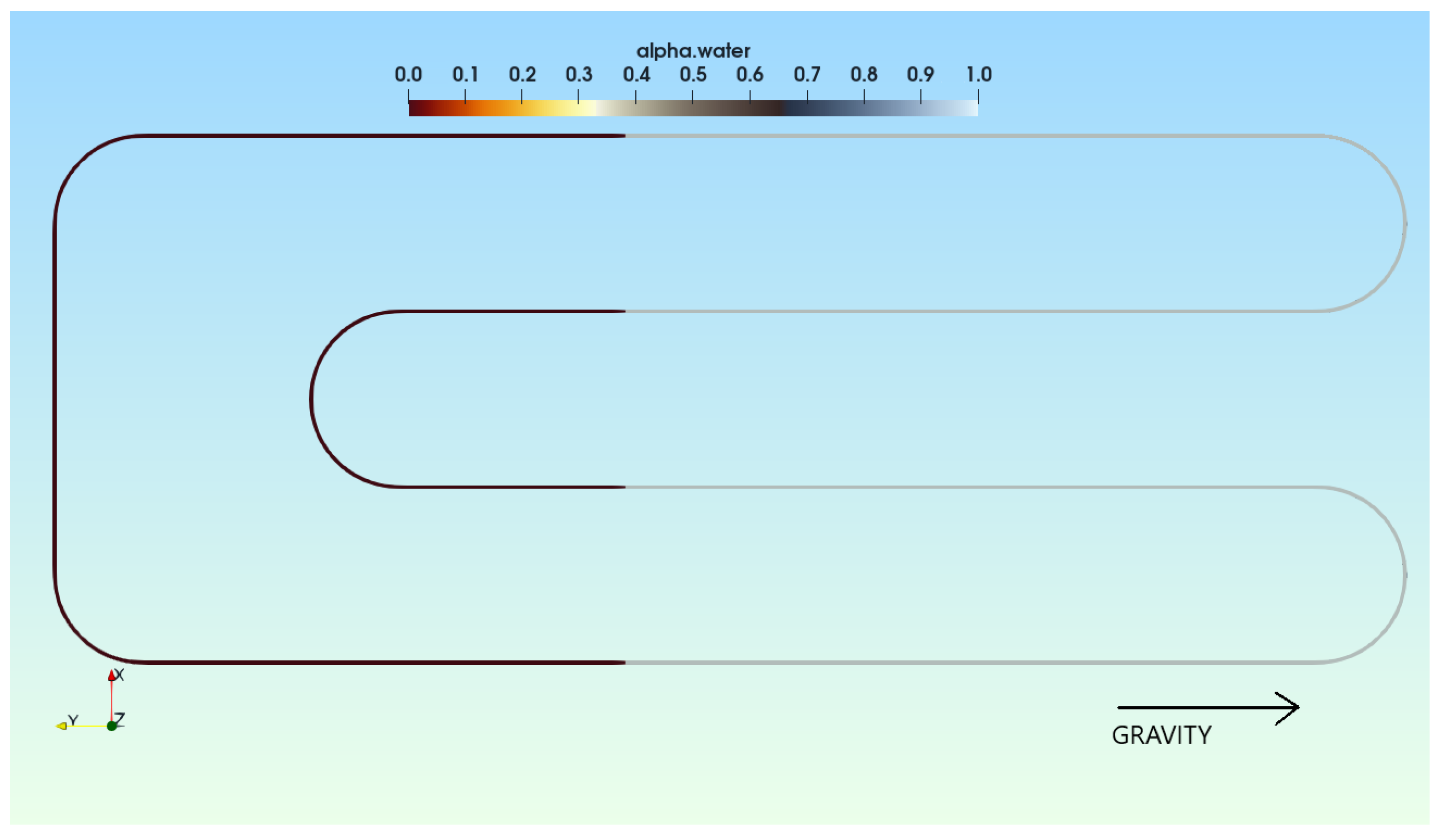
3. Numerical Modeling

The simulation uses a solver for boiling and condensation which is written in C++ programming language and is based on OpenFOAM-v1612 and the solver interPhaseChangeFoam. The simulation was performed for ethanol using four different mass transfer models with different heat fluxes acting on the PHP.

Instead of using a standard Courant number approach, the solver introduces Galusiński-Vigneaux criteria for the time step which, like the Courrant number, allows its value to maintain the stability of the simulation. The value of the entered criterion is inversely proportional to the kinematic viscosity, density, cell size, and proportional to the surface tension of the fluid [30]. Initial values of these parameters are determined like the rest of the thermophysical properties based on saturation pressure, which can be found in the summary

Table 2. Initial conditions and model settings table.

Heat Flux	Transport Model	${\mathit{p}}_{\mathbf{sat}}$	Cond. Temp.	Remarks
75 W	Kafeel and Turan (18)	5.23 kPa	288.53 K	${\beta }_c=100$, ${\beta }_v$ = 0.5
75 W	Xu (19)	5.23 kPa	288.53 K	${\beta }_c=0.1$, ${\beta }_v$ = 0.1
100 W	Tanasawa (12)	5.85 kPa	288.38 K	$\gamma$ = 1
100 W	Lee (16)	5.85 kPa	288.38 K	${\beta }_c=100$, ${\beta }_v$ = 0.5
100 W	Kafeel and Turan (18)	5.85 kPa	288.38 K	${\beta }_c=100$, ${\beta }_v$ = 0.5
100 W	Xu (19)	5.85 kPa	288.38 K	${\beta }_c=0.1$, ${\beta }_v$ = 0.1

.

An additional boundary condition for the heat flux entering the domain was also required to be introduced into the source code. The reason for this is that in the official version of OpenFOAM, it is only possible to perform heat delivery to an incompressible fluid using a fixed temperature or temperature gradient boundary conditions. In the experiment, the heat flux flowing to the domain is conveyed by the wrapped wire, which is treated as an evaporator section. To model the heat flux boundary condition, a modified heat flux boundary condition is necessary. In the classical temperature gradient boundary condition, it is assumed that the heat flowing into the domain is transferred to the domain such that it is only filled with liquid which expresses Equation (3) neglecting the heat transfer to the gas phase and the cells where the interface occurred. This is not acceptable in multiphase flow modelling. Therefore, a heat flux boundary condition which takes into account the separated temperature gradient for each phase and the cells where there is an interface between the phases, was implemented and expressed in the following formulas [19].

$$-\nabla T=\frac{q}{{{\alpha }_{l}k}_l}$$

(3)

$$-\nabla T=\frac{q}{{{\alpha }_{v}k}_v}$$

(4)

$$-\nabla T=\frac{q}{{{\alpha }_{v}k}_v+{\alpha }_l{k}_l}$$

(5)

Additionally, the use of this boundary condition allows the heat to be delivered without assuming a temperature in the evaporator section.

3.1. Governing Equations

Modelling of a two-phase flow including heat transfer requires the calculation of the behaviour of the phases and shapes of the interfaces between them. For the numerical analysis of flow inside the PHP, the liquid and vapour phases are assumed as incompressible fluids and the flow is two-dimensional. In this model, the volume of fluid (VOF) method was utilised. The volume fraction is represented by a fraction value between 0 and 1, where 0 corresponds to a cell that does not contain the “i-th” phase, whereas 1 to a cell fully filled with that phase. The tracking of the phase interface is accomplished by the solution of a continuity equation for the volume fraction of the liquid phase. Knowing the ${\alpha }_l$ the volume fraction of the vapour phase is obtained from the following equation

$${\alpha }_l+{\alpha }_v=1$$

(6)

The study uses the k-$\omega$ turbulence model, introduced by adding a thermal wall function for turbulent thermal diffusivity to the equation. Equations expressing the mass, momentum, energy, and phase equations in the VOF model are presented below.

Continuity equation for the liquid volume fraction:

$$\frac{\partial {\alpha }_l}{\partial t}+\nabla ·\left({\alpha }_l\mathbf{U}\right)+\nabla ·\left({\alpha }_l{\alpha }_v{\mathbf{U}}_r\right)-\left({\alpha }_l\nabla ·\mathbf{U}\right)=\left(J_{vl}-J_{lv}\right)\left[\frac{1}{{\rho }_l}-{\alpha }_l\left(\frac{1}{{\rho }_l}-\frac{1}{{\rho }_v}\right)\right]$$

(7)

This is an advection equation with added source terms on the right hand side that account for the phase change. In multiphase flows, it is important to obtain as sharp an interface as possible. In the present study, the algebraic method of interface compression is used [31] and the boundedness of the $\alpha$ field is assured via MULES algorithm [32]. Therefore, the third term on the left hand side is the additional term. It acts only at the interface and is responsible for compression of the interface. The ${\mathbf{U}}_r={\mathbf{U}}_l-{\mathbf{U}}_v$ is a relative velocity.

Momentum equation:

$$\begin{array}{cc}\hfill \frac{\partial \left(\rho \mathbf{U}\right)}{\partial t}+\nabla ·\left(\rho \mathbf{UU}\right)-\mathbf{U}\frac{\partial \rho }{\partial t}-\mathbf{U}\left[\nabla ·\left(\rho \mathbf{U}\right)\right]=& -\nabla p_{rgh}+\nabla ·\left[\nu \left(\nabla \mathbf{U}+\nabla {\mathbf{U}}^T\right)\right]\hfill \\ \hfill & -\mathbf{g}·\mathbf{h}\nabla \rho +\sigma \kappa \nabla {\alpha }_l\hfill \end{array}$$

(8)

The influence of the surface tension force is modelled using the continuum surface model (CSF) [33]. The occurrence of the third term on the right hand side results from the fact that the solver solves for $p_{rgh}=p-\rho \left(\mathbf{g}·\mathbf{h}\right)$ [34].

Energy equation:

$$\frac{\partial T}{\partial t}+\nabla ·\left(\mathbf{U}T\right)-T\nabla ·\mathbf{U}=\nabla ·\left(\frac{k}{\rho c_p}\nabla T\right)+\left(J_{vl}-J_{lv}\right)\frac{h_{vap}}{\rho c_p}$$

(9)

The last term on the right hand side has been added to account for the energy change due to the latent heat. In the governing equations, all variables representing the mixture properties $\phi$ (like $\rho$, $\nu$ or k) were calculated according to the linear interpolation scheme

$$\phi ={\alpha }_1{\phi }_1+{\alpha }_2{\phi }_2$$

(10)

Only the specific heat capacity $c_p$ was calculated as

$$c_p=\frac{c_{p_1}{\rho }_1{\alpha }_1+c_{p_2}{\rho }_2{\alpha }_2}{{\rho }_1{\alpha }_1+{\rho }_2{\alpha }_2}$$

(11)

3.2. Mass Transfer Models

In the paper, four mass transfer models have been compared and implemented into the code: Tanasawa [26], Lee [27], Kafeel and Turan [28] and Xu et al. [29]. Below, a brief description of each model is given.

The Tanasawa model [26] was originally elaborated for condensation modelling purposes and is shown in Equation (12). It is a simplification of the Schrage model Equation (13) by assuming a small temperature jump at the interface, the mass flux is linearly dependent on the temperature jump between phases [26]. The model is based on the kinetic theory of gases and takes into account the kinetic energy of the contributors. Fraction $\gamma$ in Equation (14) is used to define the number of molecules changing phase and transferring across the interface. It is the number of molecules transferred to the vapour phase divided by the number of molecules emitted from the liquid phase. The value of 1 corresponds to the ideal condensation where all molecules are absorbed by the liquid phase [35].

Tanasawa model

$$\dot{m}=\frac{2\gamma }{2-\gamma }\sqrt{\frac{M}{2\pi R}}\left[\frac{{\rho }_v{h}_{vap}\left(T-T_{sat}\right)}{T_{sat}^{3/2}}\right]$$

(12)

Schrage model

$$\dot{m}=\frac{2\gamma }{2-\gamma }\sqrt{\frac{M}{2\pi R}}\left[\frac{p_v}{\sqrt{T_{v,sat}}}-\frac{p_l}{\sqrt{T_{l,sat}}}\right]$$

(13)

Fraction value

$$\gamma =\frac{n_{lv}}{n_l}$$

(14)

To use mass flux $\dot{m}$ from Equation (12) in the governing equations it has to be transformed into volumetric mass transfer J. It is done by the following equation [25]

$$J=\dot{m}|\nabla {\alpha }_l|$$

(15)

The Lee model [27] is a simplified saturation model for condensation and evaporation processes. The intensity of the phase change is proportional to the temperature difference between the saturation temperature and temperature inside the domain. The model assumes that the volumetric mass transfer is expressed by the following patterns [24].

Lee model during condensation

$$J_{lv}={\beta }_c{\alpha }_v{\rho }_v\frac{T-T_{sat}}{T_{sat}}$$

(16)

Lee model during evaporation

$$J_{vl}={\beta }_v{\alpha }_l{\rho }_l\frac{T-T_{sat}}{T_{sat}}$$

(17)

The extension of the model [19,28] is based on the basic Lee model Equations (16) and (17), but it takes into account the change in the intensity of the phase transition and prevents the dryout phenomenon by correcting the ${\beta }_c$ relaxation coefficient. The appearance of dryout in the PHP results from the fact that with the heat flowing into the domain, the value of $J_{lv}$ increases in relation to $J_{vl}$. This can be prevented by correcting the value of the relaxation coefficients using Equation (18). The value of ${\beta }_v$ is kept constant.

$${\beta }_c^{n+1}={\beta }_c^n-{\beta }_c^n\left[\frac{{\sum }_{i=1}^{tot}{J}_{vl,i}-{\sum }_{i=1}^{tot}{J}_{lv,i}}{max\left({\sum }_{i=1}^{tot}{J}_{vl,i}-{\sum }_{i=1}^{tot}{J}_{lv,i}\right)}\right]$$

(18)

The Xu et al. model [29], which is similar to Equation (18), corrects the relaxation coefficients with the difference that the relaxation coefficient during evaporation ${\beta }_v$ is modified as well. In the case of the Xu et al. model, the evaporation relaxation factor is calculated based on the formula Equation (19).

$${\beta }_v^{n+1}={\beta }_v^n-{\beta }_v^n\left[\frac{{\sum }_{i=1}^{tot}{J}_{lv,i}-{\sum }_{i=1}^{tot}{J}_{vl,i}}{max\left({\sum }_{i=1}^{tot}{J}_{vl,i}-{\sum }_{i=1}^{tot}{J}_{lv,i}\right)}\right]$$

(19)

3.3. Numerical Details

The mesh was made on the basis of the setup presented in Figure 1. All dimensions were kept as in reality. The mesh was generated using ANSYS Meshing [36]. The boundary layer and the number of elements were selected on the basis of mesh independence studies, see Figure 2, where the effect of element size on the condenser surface heat flux was investigated. Thus, a mesh with an element size of 0.5 mm was decided to be used. Only the first milliseconds of the simulation were investigated in terms of mesh independence because longer simulations would be computationally intensive and the discrepancy between them due to sensitivity to initial conditions would be significant.

The generated mesh (Figure 3) has an average orthogonal quality of 0.99, while an average skewness value of 2.5 × 10${}^{-2}$ was obtained. The boundary layer was created due to the fact that turbulent flow was assumed inside the pipes. To make the simulation more realistic, the boundary condition of the heat flux flowing into the domain was made in such a way that it resembled a wire wound on the PHP. The value on the basis of which the fluid parameters were calculated was the saturation pressure. The pressure measurement showed the greatest accuracy and it was on the basis of this value that the remaining parameters were read on the basis of the CoolProp [37] library. The boundary condition for the fluid distribution is shown in Figure 4. The tube filling ratio value was 52.62% and corresponded to the value in the laboratory experiment. The time step value was generated based on the Galusiński-Vigneaux criterion number equaling 40 for each case, it was sufficient to get the stability of the simulation. The resulting time steps varied from 1.5 × 10${}^{-6}$ to 3 × 10${}^{-6}$ s depending on the current state of the simulation. The residual values were assumed to be 1 × 10${}^{-10}$ except for momentum, for which the value was set to 1 × 10${}^{-8}$. The initial conditions and the adopted transport models are presented in summary in Table 2.

In the simulation, for the calculation of the time differential, the Euler scheme was used, a Gauss van Leer was used for divergence calculations, expecting the divergence in turbulence equations, where a Gauss linear was employed. For laplacians and gradients, a Gauss linear scheme was used.

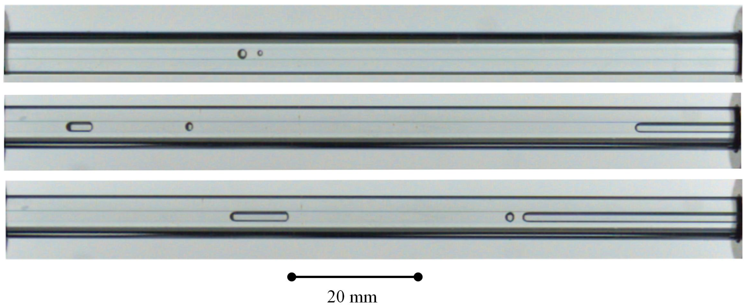
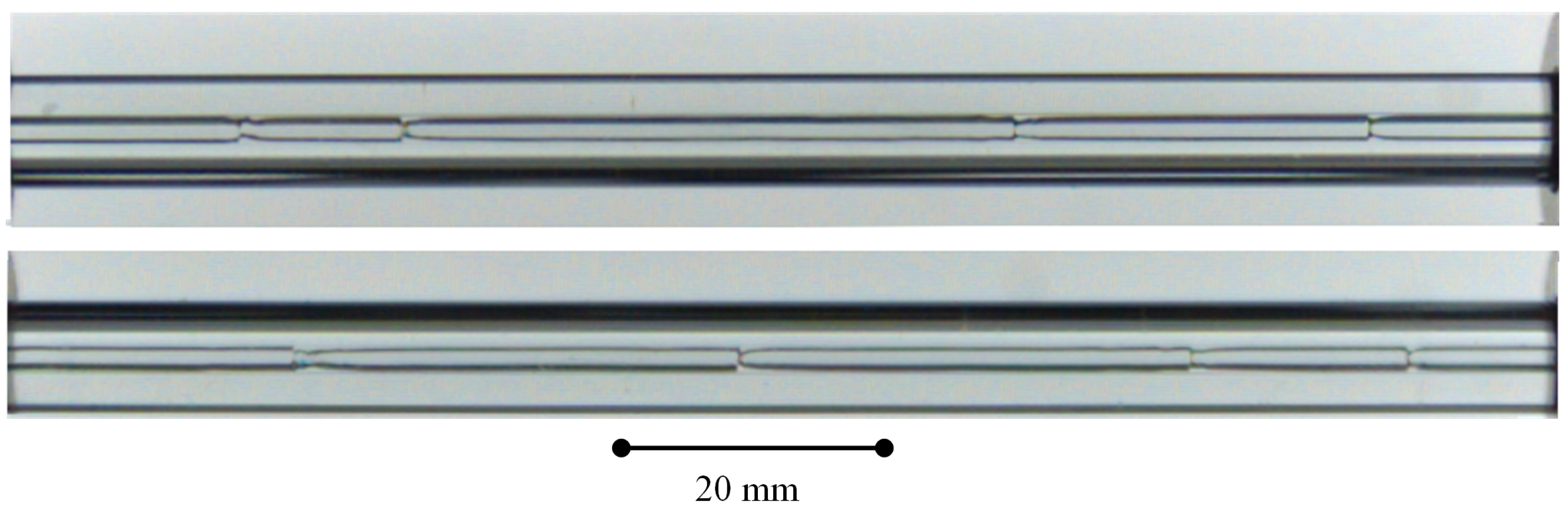
4. Results and Discussion

The purpose of the numerical analysis was to capture the formation of characteristic flow structures and compare them with experimentally observed ones. It was aimed at obtaining a higher resolution than the predecessors preceding, whose goal was to present the phenomenon of pulsation as, e.g., in the work of Pouryoussefi and Zhang [38], rather than to reproduce the detailed boiling structures of the fluid inside the pipe. This part shows the results of laboratory experiments recorded with a multiframe camera and compares them with structures generated numerically by different phase change models.

4.1. Experimental Results

This subsection shows the common fluid structures captured by a high-speed camera. Ethanol was charged at 52.6% filling ratio and all presented flow structures were from the experimental run at power 100 W on the evaporator coil. During the experimental run of 600 s, the temperature range for the condenser region was 14.63–19.2 °C and for evaporator region it was between 32.97–48.46 °C. Figure 5 shows characteristic vapour plugs ending in the meniscus that become more convex the faster moves. In each case of capturing vapour plugs inside the pipe, the meniscuses are convex. In Figure 5, the plugs move in a left to right direction. It can be seen that the angle of the meniscus is different on each side of the plug and depends on both speed and direction. The higher the interface displacement over time caught by the high-speed camera, the greater the angle and the more convex the meniscus. The greater convexity is always found on the front face of the plug.

It is worth noting that the structures inside the pipes do not resemble a sphere, and most plugs, even when moving at a slight speed, resemble a lens rather than a circle. From the perspective of assessing the effectiveness of the numerical model, this should be taken into account. Figure 6 shows an example of isolated small structures resembling a lens.

However, the most commonly observed flow structures are substrate plugs locally perturbed by accumulating liquid running off the boundary layer. In Figure 7, one of the two most common shapes within the PHP is shown, which consists of individual plugs connected to each other by adhesion forces composing the elongated bubble regime. To capture these structures in the numerical model, a prismatic mesh with higher resolution near the wall was created and a turbulence model was adopted to realise the numerically generated structures, which is shown in Section 4.2.

The elongated bubble flow often results in the irregular merging of plug structures, which is shown in Figure 8. It shows the necessity of a boundary layer in the simulation and the use of a turbulence model. The inclusion of turbulence allows the modelling of such irregularities resulting from the influence of the wall as well as the local appearance of condensates. As these structures appear in the adiabatic section, it may be concluded that the main reason for such irregularities is the wall influence and differences in viscous forces within the phases.

The next recurrent structure is that shown in Figure 9. It is a fully annular flow regime. It occurs as frequently as the structure shown in Figure 7, except that it occurs at much higher velocities inside the pipe. It is noticeable that there is a boundary layer on which the liquid slug condenses, causing turbulence in the vapour plug flow that is visible by the waves at the plug surface.

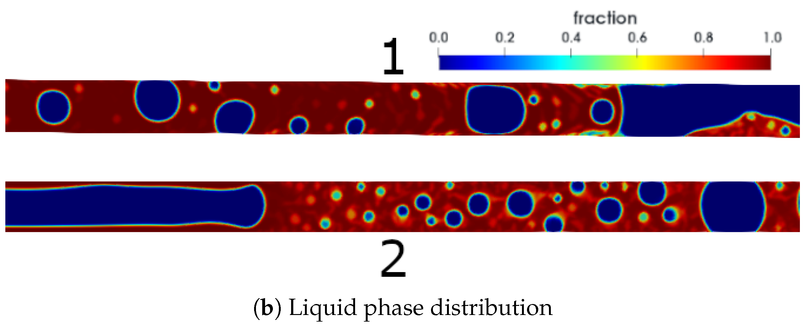
4.2. Numerical Results

Figure 10, Figure 11, Figure 12 and Figure 13 show the dynamics and shape of the formation of the bubble-shaped structures in the first milliseconds of the simulation for the four mass transfer models. As can be seen, each mass transfer model gives different flow structures. This results from both distinct bases of the models (gas kinetic theory for the Tanasawa model and temperature difference for the Lee family model) and the diverse relaxation factors applied. The least intense phase transformation occurs with the Xu model (Figure 10). This is determined by the relaxation factors, which affect the evaporation rate and, unlike the other mass transfer models, also affect the condensation. The fastest phase change occurs with the Tanasawa model (Figure 11). This model does not prevent dryout, in the presented figure, it can be seen that the generated shapes do not form single bubble structures, which are visible in the experiment shown in Figure 6. The generated structures are symmetric to each other and the interface between the phases is unnaturally sharp when comparing them to those from the Chirag et al. paper [35]. There is a strong similarity between the Lee model (Figure 12) and the Kafeel and Turan model (Figure 13), due to the fact that both models assume a constant relaxation factor for evaporation. However, all models show the formation of vapour plugs, with the characteristic convexity of the meniscus occurring in reality.

The selection of results in the model was guided by the most common structures found in the simulation. Figure 14 shows the distribution of the fluid inside the domain for the Tanasawa model. It is possible to notice the similarity of the ethanol slug-plug flow regime to the experiment presented in Figure 5. Vapour plugs have a convex meniscus at the end and the transfer of molecules between them occurs only in larger structures. In the simulation with the Tanasawa model, the solver does not generate a thin liquid boundary layer in the region where the fluid locally accelerates. This results in a lack of structures where liquid does not drip from the wall and accumulate on it in the form of larger condensates, as in the experiment (Figure 7). This has implications for no separation of larger plugs into smaller sharpened vapour plugs. In Figure 15b it can be noticed a considerably enlarged boundary layer, which does not exist in the experiment and can be considered as a calculation error. The model requires the least computational resources compared to the other three models. With the model, we can get a relatively good approximation of the real flow structure, characteristic of the model is a flow dominated by vapour plugs rather than a multitude of individual bubbles. In longer simulations, proper selection of the $\gamma$ coefficient is required (Equation (14)), because it is the only modifiable factor that prevents dryout inside the pipe and maintaining the quasi-steady pulsating state.

The Lee model results are shown in Figure 16 and Figure 17. The simulation imitates the plug and slug structures, as in the Tanasawa model (Figure 14 and Figure 15), but there is a transfer between them based on smaller bubble structures. It occurs in the experiment but is not as extensive, and it is not the dominant transfer of molecules from one plug to another. The dominant factor which connects these structures is the effect of adhesion forces, which can be seen in Figure 7. In this experiment, there are no irregular bubbles breaking away from larger structures, neither of these irregular structures are shown in Figure 8. The main difference between the model and reality is the presence of such small liquid slugs (Figure 17b), which in reality would interact with each other by adhesion forces.

The next presented transport model is the Kafeel and Turan model [28]. Results for two different heat powers are presented in Figure 18, Figure 19 and Figure 20 to verify the effect of process intensity on the generated fluid structures. As in the Lee model, the vapour ethanol bubbles are the dominant flow regime between vapour plugs. Small ethanol slug structures are less frequent as in the Lee model. At the higher heat power (Figure 20), a more regular flow with a formed wall layer is observed. The vapour bubbles gain a meniscus only if in contact with the surface of a heat pipe, as observed in reality. In the numerical model, the frequency of occurrence of such structures in the simulation is much higher than in the case captured by the camera. The increased heat power influences the initial movement of the fluid structures, however, in the long term, it has no impact on the dynamics of fluid movement inside the PHP.

The phase change model that best reflected the fluid structure of the experiment was the Xu model [29]. Simulations for the Xu model were performed in two variants—75 and 100 W. The results from which a high similarity of structures can be recognised are presented below. The structures in Figure 21b are likewise similar to those in Figure 7, with the visible boundary layer and the way the vapour plugs are connected similarly to those in Figure 8. The imperfection of the model is that there are quite a lot of small bubbles that break away from the vapour plugs as observed in Figure 22b. The difference between the single plugs in Xu’s model, as opposed to Lee’s or Kafeel-Turan’s, is that their shape is composed of not only convex meniscuses, but also concave ones, as shown in Figure 23b. As with the smaller heat power, the merging of the vapour slugs occurs in a way similar to that of the experiment.

4.3. Comparison of the Experimental and Numerical Velocities

Not every detail can be captured with multiframe cameras, such as the velocity vectors inside the vapour plugs. The figure below shows the distribution of vectors inside the vapour bubbles. In Figure 24 it can be seen that the highest velocities occur inside the vapour structures, where the flow within the bubble accelerates, as can be seen in Figure 7 or Figure 9. In Figure 24 it is presented the slow merging of vapour plugs. In local laminar flow, the velocity vectors are largest in the middle of the pipe, closer to the wall velocity decreases.

The vectors that can be obtained in the experiment are shown below. For this purpose, the particle image velocimetry (PIV) software [39] has been used. It allows for the tracking of the interfacing between phases and for determining the velocity expressed graphically as green arrows. Between 20 and 100 frames of video were used to generate the velocity vectors in the PIV software [40]. The number of pixels per length of the observable area was determined, and from this value the conversion factor pixel to meter was calculated. The PIV algorithm enabled the calculation of the interface speed value. After taking into account this coefficient, the results were converted to the SI system of units. A comparable image referenced by the PIV analysis is shown in Figure 25. The velocity values, from experiment, shown in Figure 26 are on average 0.075 m/s, which is a very comparable to value obtained numerically. The discrepancy between the values obtained at the edges of the interface in the slug-plug flow is of the order of 10%. In the case of turbulent flow, these values are overestimated relative to the experiment, the velocity values. However, in the case of turbulent flow, the results should be evaluated in terms of order of magnitude rather than values, because the range of occurrence of such structures and the corresponding velocities in this case are wide. In the turbulent flow algorithm managed to capture the interface velocity in the wall layer (Figure 27), it was 0.105 m/s.

5. Conclusions

The above work presents the results of a numerical analysis of pulsating heat pipes. It was possible to present and compare the results of the numerical analysis with the experiment. The experiments were performed on a specially designed test stand where visualisation of the flow structures could be done. The numerical simulations have been carried out in OpenFOAM software where the code for two-phase flow with phase change has been implemented. The influence of the mass transport model on the dynamics and shape of the generated structures was shown. Based on the obtained results, the following findings are made:

• Using implemented algorithm it was possible to capture the structures of the fluid, which closely resembled those gained during the experiments in the laboratory.
• The phase change models based on the Lee model [27,28,29] give different flow structures showing that the relaxation coefficients highly influence the results.
• For the analysed case, the most optimal model of the phase change was the Xu et al. [29] model was the best model that reflected reality.

The continuation of the work can certainly be the creation of a 3D model based on the Xu model and the determination of structures in space. The work could also be continued by improving the solver which would use the level set coupled with the VOF method, enable conjugate heat transfer, and reduce spurious current. In the future, for comparing the effectiveness of PHP modeling, it would be a good idea to build a simplified laboratory stand from a pipe made of one loop and a wider diameter. This would allow a reduction in the number of computational possibilities required and a better observation of the pulsation itself.

References

1. Smakulski, P.; Pietrowicz, S. A review of the capabilities of high heat flux removal by porous materials, microchannels and spray cooling techniques. Appl. Therm. Eng. 2016, 104, 636–646. [Google Scholar] [CrossRef]
2. Czajkowski, C.; Nowak, A.I.; Błasiak, P.; Ochman, A.; Pietrowicz, S. Experimental study on a large scale pulsating heat pipe operating at high heat loads, different adiabatic lengths and various filling ratios of acetone, ethanol, and water. Appl. Therm. Eng. 2020, 165, 114534. [Google Scholar] [CrossRef]
3. Czajkowski, C.; Nowak, A.I.; Pietrowicz, S. Flower Shape Oscillating Heat Pipe—A novel type of oscillating heat pipe in a rotary system of coordinates—An experimental investigation. Appl. Therm. Eng. 2020, 179, 115702. [Google Scholar] [CrossRef]
4. Czajkowski, C.; Błasiak, P.; Rak, J.; Pietrowicz, S. The development and thermal analysis of a U-shaped pulsating tube operating in a rotating system of coordinates. Int. J. Therm. Sci. 2018, 132, 645–662. [Google Scholar] [CrossRef]
5. Yang, P.; Zhang, Y.; Wang, X.; Liu, Y.W. Heat transfer measurement and flow regime visualization of two-phase pulsating flow in an evaporator. Int. J. Heat Mass Transf. 2018, 127, 1014–1024. [Google Scholar] [CrossRef]
6. Wojtan, L.; Ursenbacher, T.; Thome, J.R. Investigation of flow boiling in horizontal tubes: Part I—A new diabatic two-phase flow pattern map. Int. J. Heat Mass Transf. 2005, 48, 2955–2969. [Google Scholar] [CrossRef]
7. Nikolayev, V.S. Physical principles and state-of-the-art of modeling of the pulsating heat pipe: A review. Appl. Therm. Eng. 2021, 195, 117111. [Google Scholar] [CrossRef]
8. Kholi, F.K.; Mucci, A.; Kallath, H.; Ha, M.Y.; Chetwynd-Chatwin, J.; Min, J.K. An improved correlation to predict the heat transfer in pulsating heat pipes over increased range of fluid-filling ratios and operating inclinations. J. Mech. Sci. Technol. 2020, 34, 2637–2646. [Google Scholar] [CrossRef]
9. Mucci, A.; Kholi, F.K.; Chetwynd-Chatwin, J.; Ha, M.Y.; Min, J.K. Numerical investigation of flow instability and heat transfer characteristics inside pulsating heat pipes with different numbers of turns. Int. J. Heat Mass Transf. 2021, 169, 120934. [Google Scholar] [CrossRef]
10. Wang, J.; Ma, H.; Zhu, Q. Effects of the evaporator and condenser length on the performance of pulsating heat pipes. Appl. Therm. Eng. 2015, 91, 1018–1025. [Google Scholar] [CrossRef]
11. Ghanta, N.; Pattamatta, A. Modeling of compressible phase-change heat transfer in a Taylor-Bubble with application to pulsating heat pipe (PHP). Numer. Heat Transf. Part A Appl. Int. J. Comput. Methodol. 2016, 69, 1355–1375. [Google Scholar] [CrossRef]
12. Wang, J.; Ma, H.; Zhu, Q.; Dong, Y.; Yue, K. Numerical and experimental investigation of pulsating heat pipes with corrugated configuration. Appl. Therm. Eng. 2016, 102, 158–166. [Google Scholar] [CrossRef]
13. Dang, C.; Jia, L.; Lu, Q. Investigation on thermal design of a rack with the pulsating heat pipe for cooling CPUs. Appl. Therm. Eng. 2017, 110, 390–398. [Google Scholar] [CrossRef]
14. Pouryoussefi, S.; Zhang, Y. Analysis of chaotic flow in a 2D multi-turn closed-loop pulsating heat pipe. Appl. Therm. Eng. 2017, 126, 1069–1076. [Google Scholar] [CrossRef] [Green Version]
15. Venkata, J.; Bhramara, P. CFD Analysis of Copper Closed Loop Pulsating Heat pipe. Mater. Today Proc. 2018, 5, 5487–5495. [Google Scholar] [CrossRef]
16. Wang, J.; Bai, X. The features of CLPHP with partial horizontal structure. Appl. Therm. Eng. 2018, 133, 682–689. [Google Scholar] [CrossRef]
17. Li, Q.; Wang, Y.; Lian, C.; Li, H.; He, X. Effect of micro encapsulated phase change material on the anti-dry-out ability of pulsating heat pipes. Appl. Therm. Eng. 2019, 159, 113854. [Google Scholar] [CrossRef]
18. Sagar, K.; Naik, H.; Mehta, H. CFD Analysis of Cryogenic Pulsating Heat Pipe with Near Critical Diameter under Varying Gravity Conditions. Theor. Found. Chem. Eng. 2020, 54, 64–76. [Google Scholar] [CrossRef]
19. Choi, J.; Zhang, Y. Numerical simulation of oscillatory flow and heat transfer in pulsating heat pipes with multi-turns using OpenFOAM. Numer. Heat Transf. Part A Appl. Int. J. Comput. Methodol. 2020, 77, 761–781. [Google Scholar] [CrossRef]
20. Barba, M.; Bruce, R.; Baudouy, B. Numerical simulation of the thermal and fluid-dynamic behavior of a cryogenic capillary tube. Cryogenics 2020, 106, 103044. [Google Scholar] [CrossRef]
21. Xie, F.; Li, X.; Qian, P.; Huang, Z.; Liu, M. Effects of geometry and multisource heat input on flow and heat transfer in single closed-loop pulsating heat pipe. Appl. Therm. Eng. 2020, 168, 114856. [Google Scholar] [CrossRef]
22. Vo, D.T.; Kim, H.T.; Ko, J.; Bang, K.H. An experiment and three-dimensional numerical simulation of pulsating heat pipes. Int. J. Heat Mass Transf. 2020, 150, 119317. [Google Scholar] [CrossRef]
23. Wang, W.W.; Wang, L.; Cai, Y.; Yang, G.B.; Zhao, F.Y.; Liu, D.; Yu, Q.H. Thermo-hydrodynamic model and parametric optimization of a novel miniature closed oscillating heat pipe with periodic expansion-constriction condensers. Int. J. Heat Mass Transf. 2020, 152, 119460. [Google Scholar] [CrossRef]
24. Li, Q.; Wang, C.; Wang, Y.; Wang, Z.; Li, H.; Lian, C. Study on the effect of the adiabatic section parameters on the performance of pulsating heat pipes. Appl. Therm. Eng. 2020, 180, 115813. [Google Scholar] [CrossRef]
25. Hardt, S.; Wondra, F. Evaporation model for interfacial flows based on a continuum-field representation of the source terms. J. Comput. Phys. 2008, 227, 5871–5895. [Google Scholar] [CrossRef]
26. Tanasawa, I. Advances in Condensation Heat Transfer. Adv. Heat Transf. 1991, 21, 55–139. [Google Scholar] [CrossRef]
27. Lee, W. A Pressure Iteration Scheme for Two-Phase Flow Modeling. In Computational Methods for Two-Phase Flow and Particle Transport; World Scientific Publishing Company: Singapore, 2013; pp. 61–82. [Google Scholar] [CrossRef]
28. Kafeel, K.; Turan, A. Axi-symmetric simulation of a two phase vertical thermosyphon using Eulerian two-fluid methodology. Heat Mass Transf. 2013, 49, 1089–1099. [Google Scholar] [CrossRef]
29. Xu, Z.; Zhang, Y.; Li, B.; Huang, J. Modeling the phase change process for a two-phase closed thermosyphon by considering transient mass transfer time relaxation parameter. Int. J. Heat Mass Transf. 2016, 101, 614–619. [Google Scholar] [CrossRef]
30. Galusinski, C.; Vigneaux, P. On stability condition for bifluid flows with surface tension: Application to microfluidics. J. Comput. Phys. 2008, 227, 6140–6164. [Google Scholar] [CrossRef] [Green Version]
31. Berberović, E.; van Hinsberg, N.P.; Jakirlić, S.; Roisman, I.V.; Tropea, C. Drop impact onto a liquid layer of finite thickness: Dynamics of the cavity evolution. Phys. Rev. E 2009, 79, 036306. [Google Scholar] [CrossRef]
32. Weller, H. A New Approach to Vof-Based Interface Capturing Methods for Incompressible and Compressible Flow—Report TR/HGW/04; Technical Report; OpenCFD Ltd.: Bracknell, UK, 2008. [Google Scholar]
33. Brackbill, J.; Kothe, D.; Zemach, C. A continuum method for modeling surface tension. J. Comput. Phys. 1992, 100, 335–354. [Google Scholar] [CrossRef]
34. OpenFOAM: User Guide v2012. 2020. Available online: https://www.openfoam.com/documentation/user-guide (accessed on 14 August 2021).
35. Chirag, R.; Kharangate, I.M.; Mudawa, I. Review of computational studies on boiling and condensation. Int. J. Heat Mass Transf. 2017, 108, 1164–1196. [Google Scholar] [CrossRef]
36. Ansys®. Academic Research Meshing, Release 2021 R2. Available online: https://www.ansys.com/ (accessed on 14 August 2021).
37. Bell, I.H.; Wronski, J.; Quoilin, S.; Lemort, V. Pure and Pseudo-pure Fluid Thermophysical Property Evaluation and the Open-Source Thermophysical Property Library CoolProp. Ind. Eng. Chem. Res. 2014, 53, 2498–2508. [Google Scholar] [CrossRef] [Green Version]
38. Pouryoussefi, S.; Zhang, Y. Numerical investigation of chaotic flow in a 2D closed-loop pulsating heat pipe. Appl. Therm. Eng. 2016, 98, 617–627. [Google Scholar] [CrossRef]
39. Taylor, Z.; Gurka, R.; Kopp, G.; Liberzon, A. Long-Duration Time-Resolved PIV to Study Unsteady Aerodynamics. Instrum. Meas. IEEE Trans. 2011, 59, 3262–3269. [Google Scholar] [CrossRef]
40. Thielicke, W.; Stamhuis, E. PIVlab—Towards User-friendly, Affordable and Accurate Digital Particle Image Velocimetry in MATLAB. J. Open Res. Softw. 2014, 2, e30. [Google Scholar] [CrossRef] [Green Version]
Figure 1. Experimental set-up.
Energies 14 05952 g001
Figure 2. The results of mesh independence study for heat flux on the condenser surface.
Energies 14 05952 g002
Figure 3. Generated mesh.
Energies 14 05952 g003
Figure 4. Initial distribution of ethanol for each case.
Energies 14 05952 g004
Figure 5. Plug-slug flow regime captured by high speed camera in the adiabatic section for the case of 100 W input power and ethanol as working fluid—52.6% filling ratio.
Energies 14 05952 g005
Figure 6. Examples of lens-shaped fluid structures captured in the adiabatic section for the 100 W input power and ethanol as working fluid—52.6% filling ratio.
Energies 14 05952 g006
Figure 7. Common structure of elongated bubbles regime in the adiabatic section for the case of 100 W input power and ethanol as working fluid—52.6% filling ratio.
Energies 14 05952 g007
Figure 8. Merging of plug structures in the elongate bubble flow regime inside the PHP for the case of 100 W input power and ethanol as working fluid—52.6% filling ratio.
Energies 14 05952 g008
Figure 9. Annular flow regime inside the PHP for the case of 100 W input power and ethanol as working fluid—52.6% filling ratio.
Energies 14 05952 g009
Figure 10. The distribution of ethanol volume fraction (alpha.water) in the evaporator area for the first milliseconds of simulation in the Xu et al. [29] mass transport model for the case of 100 W input power.
Energies 14 05952 g010
Figure 11. The distribution of ethanol volume fraction (alpha.water) in the evaporator area for the first milliseconds of simulation in the Tanasawa [26] mass transport model for the case of 100 W input power.
Energies 14 05952 g011
Figure 12. The distribution of ethanol volume fraction (alpha.water) in the evaporator area for the first milliseconds of simulation in the Lee [27] mass transport model for the case of 100 W input power.
Energies 14 05952 g012
Figure 13. The distribution of ethanol volume fraction (alpha.water) in the evaporator area for the first milliseconds of simulation in the Kafeel and Turan [28] mass transport model for the case of 100 W input power.
Energies 14 05952 g013
Figure 14. Numerical results of the Tanasawa model [26] in 0.2 s for 100 W input power.
Energies 14 05952 g014
Figure 15. Numerical results of the Tanasawa model [26] in 1.0 s for 100 W input power.
Energies 14 05952 g015
Figure 16. Numerical results of the Lee model [27] in 0.5 s for 100 W input power.
Energies 14 05952 g016
Figure 17. Numerical results of the Lee model [27] in 1.0 s for 100 W input power.
Energies 14 05952 g017
Figure 18. Numerical results of the Kafeel and Turan model [28] model in 0.5 s for 75 W input power.
Energies 14 05952 g018aEnergies 14 05952 g018b
Figure 19. Numerical results of the Kafeel and Turan model [28] model in 1.0 s for 75 W input power.
Energies 14 05952 g019
Figure 20. Numerical results of the Kafeel and Turan model [28] model in 1.0 s for 100 W input power.
Energies 14 05952 g020aEnergies 14 05952 g020b
Figure 21. Numerical results of the Xu model [29] in 0.2 s for 75 W input power.
Energies 14 05952 g021
Figure 22. Numerical results of the Xu model [29] in 0.5 s for 100 W input power.
Energies 14 05952 g022
Figure 23. Numerical results of the Xu model [29] in 0.15 s for 100 W input power.
Energies 14 05952 g023
Figure 24. Distribution of velocity vector along the pipe with turbulent flow in the Xu model, speed expressed in m/s.
Energies 14 05952 g024
Figure 25. Distribution of velocity vector along the pipe in the Xu model, speed expressed in m/s.
Energies 14 05952 g025
Figure 26. Distribution of velocity vector along the pipe in the experiment with 100 W input power and ethanol as working fluid—52.6% filling ratio.
Energies 14 05952 g026
Figure 27. Distribution of velocity vector along the pipe in the experiment with 100 W input power in turbulent flow and ethanol as working fluid—52.6% filling ratio.
Energies 14 05952 g027