Performance Evaluation of Forecasting Strategies for Electricity Consumption in Buildings

Abstract

In this paper, three main approaches (univariate, multivariate and multistep) for electricity consumption forecasting have been investigated. In fact, three major algorithms (XGBOOST, LSTM and SARIMA) have been evaluated in each approach with the main aim to figure out which one performs the best in forecasting electricity consumption. The motivation behind this work is to assess the forecasting accuracy and the computational time/complexity for an embedded forecasting and model training at the smart meter level. Moreover, we investigate the deployment of the most efficient model in our platform for an online electricity consumption forecasting. This solution will serve for deploying predictive control solutions for efficient energy management in buildings. As a proof of concept, an already existing public dataset has been used. These data were mainly collected thanks to the usage of already deployed sensors. These provide accurate data related to occupancy (e.g., presence) as well as contextual data (e.g., disaggregated electricity consumption of equipment). Experiments have been conducted and the results showed the effectiveness of these algorithms, used in each approach, for short-term electricity consumption forecasting. This has been proved by performance evaluation and error calculations. The obtained results mainly shed light on the challenging trade-off between embedded forecasting model training and processing for being deployed in smart meters for electricity consumption forecasting.

1. Introduction

During the last few decades, big importance has been given to electric load prediction and forecasting. It represents an important parameter used by many electric utilities for optimal planning and operational decisions. However, it was noticed that the level of management of these utilities has shifted from large-scale management of the entire grid to a small household level scale. This is mainly due to: (i) an energy market transition from centralized electricity production to decentralized or distributed production, and (ii) the load control, which is required for demand-side management [1]. Nevertheless, accurate load forecasting for limited population sizes (e.g., residential buildings or dwellings) is much more complicated because of the high volatility of data, related to the electricity usage [2]. In fact, the non-linearity of household consumption data and rapid fluctuations are caused by many exogenous factors, such as occupants’ behavior, the impact of calendar periods and the uncertainty of weather information [3,4].

A significant prerequisite for smart energy management is the identification of effective models for forecasting electricity power usage. This identification of load forecasting techniques is not limited to the most famous forecasting models being implemented, but in particular to the most suitable and efficient model for the specificity of each case study. Recently, the classification of load forecasting methods in response to very specific problematic has been specifically investigated in accordance to their suited methodologies [5]. The classification of techniques, mainly used for load forecasting, is primarily based on two fields. The first is related to the forecast horizons (i.e., short, medium, long), while the second corresponds to the techniques’ category (e.g., probabilistic, deterministic). For instance, unlike deterministic, probabilistic techniques provide information on uncertainties, which are related to the expected values. According to their importance in the planning and operational behavior of energy systems [6], these probabilistic methods have recently gained popularity, especially with their adaptability to the emerging context, mainly the integration of renewable energy systems. On the other hand, current research work has recently focused on an alternative methodology for increasing forecasting accuracy, which involves combining the best features of multiple single models and hybridizing them to compensate for the drawbacks of individual methods. For instance, the authors in [7] propose a hybrid architecture for short and long-term energy prediction for residential and commercial sectors. Convolutional LSTM was used for data extraction and encoding, whereas bidirectional LSTM is utilized for decoding and learning sequential patterns. This technique significantly improves forecasting performance when compared to benchmarking single methods (

Table 1. Forecasting methods for different application domains.

Ref.	Forecasting Method				Application Domain
	Univariate	Multivariate	One-Step	Multistep
[8]			SARIMA		Electricity consumption
[9]		ANN			District energy management
[10]				Nonlinear ANN	Wind Forecasting
[11]	ARIMA_KNN SVR_RF				Solar power generation
[12]			ARIMA		Micro-Grid Systems
[13]				RNN_CNN SARIMAX	Commercial buildings load
[14]				LSTM (MISO) & (MIMO)	HVAC systems
[15]				SVR XGBOOST	District heat systems
[16]	ANN				Energy demand forecasting

).

Nowadays, loads forecasting in households are becoming more and more crucial in order to manage electric consumption of equipment while ensuring energy efficiency. For instance, a forecasting approach based on unsupervised clustering technique was introduced in [17]. The authors in [18] also investigated, using the Kalman Filter method, the effect of sampling intervals on prediction accuracy. Moreover, several studies require, as a starting point, applying classification techniques before proceeding to the forecasting of electricity consumption. The aim was to address the irregularity of household electricity data. For instance, we can start by mentioning the dynamic time warping techniques [19] for clustering related energy consumption curves according to their shapes. Besides, the availability of detailed information on energy consumption, as a result of the recent deployment of domestic smart metering infrastructures [20], has facilitate grouping and clustering consumers’ common consumption habit [21]. In particular, these clustering techniques help in detecting typical consumption patterns, which considerably enhance the overall performance [22]. Last but not least, other approaches were presented in [23,24] for solving irregularity issues. The first one is based on a frequency decomposition using the wavelet technique in order to differentiate the regular load pattern from noisy components. As for the second, it is based on the Fourier’s transform method for extracting the frequency components of household consumption data, which are required to cluster the most relevant periodic patterns.

In order to anticipate energy consumption, for better home energy management, it is primordial to predict the usage of appliances in dwellings [25]. Besides, integrating the usage patterns of appliances instead of the usage of standard non-intrusive load monitoring (NILM) techniques, based on only gathered measurement, is advised to improve the load forecast performances. On the other hand, another NILM-based method consisting of forecasting the consumption of each household’s appliance separately, then regrouping them to have a forecast of aggregate accurate consumption, has been proposed in [26].

The strategies discussed in the literature for load forecasting are univariate, multivariate, one-step, multistep ahead, as shown in Table 1. The forecast of future values relies uniquely on its previous historical data in the univariate approach. The multivariate one, however, takes into account additional features, which are usually referred to as explanatory variables. Besides, several studies addressed load forecasting at the next time step, usually known as one step ahead. Forecasting several steps in the future, however, remains an open challenge.

This article proposes a comparison of various time series forecasting methods and approaches using empirical evaluation. Different approaches are used to forecast household load. The first one, which is the univariate approach, consists of the prediction of the house’s aggregated power consumption using the historical total power data for the horizons of one step ahead. Besides, the second approach (i.e., the multivariate approach) concerns the forecasting of the house’s total power consumption for one step ahead but by using the appliances’ disaggregated power data as inputs. Finally, the third approach (i.e., the multistep approach) concerns the prediction of the house’s aggregated power data for multiple steps ahead. Therefore, two main contributions of the current work from the literature are summarized as follows:

• Investigation of the three approaches, univariate, multivariate and multistep, for efficient load forecasting.
• A comparative analysis of three representative algorithms: LSTM, SARIMA and XGBOOST, have been examined in terms of accuracy and computational time/complexity.

This study aims to investigate load forecasting methods, which could be used for real-time prediction and context-driven control of building appliances. It will help selecting the most suitable method for being deployed in our platform for energy management and predictive control.

The reminder of this paper is organized as follows: Section 2 presents a brief classification of existing forecasting methods. Section 3 presents methods and materials including the used dataset, its preprocessing, together with features engineering, approaches and methods used for house’s power consumption. Section 4 presents the results and discussion. Conclusions and perspectives of this work are given in Section 5.

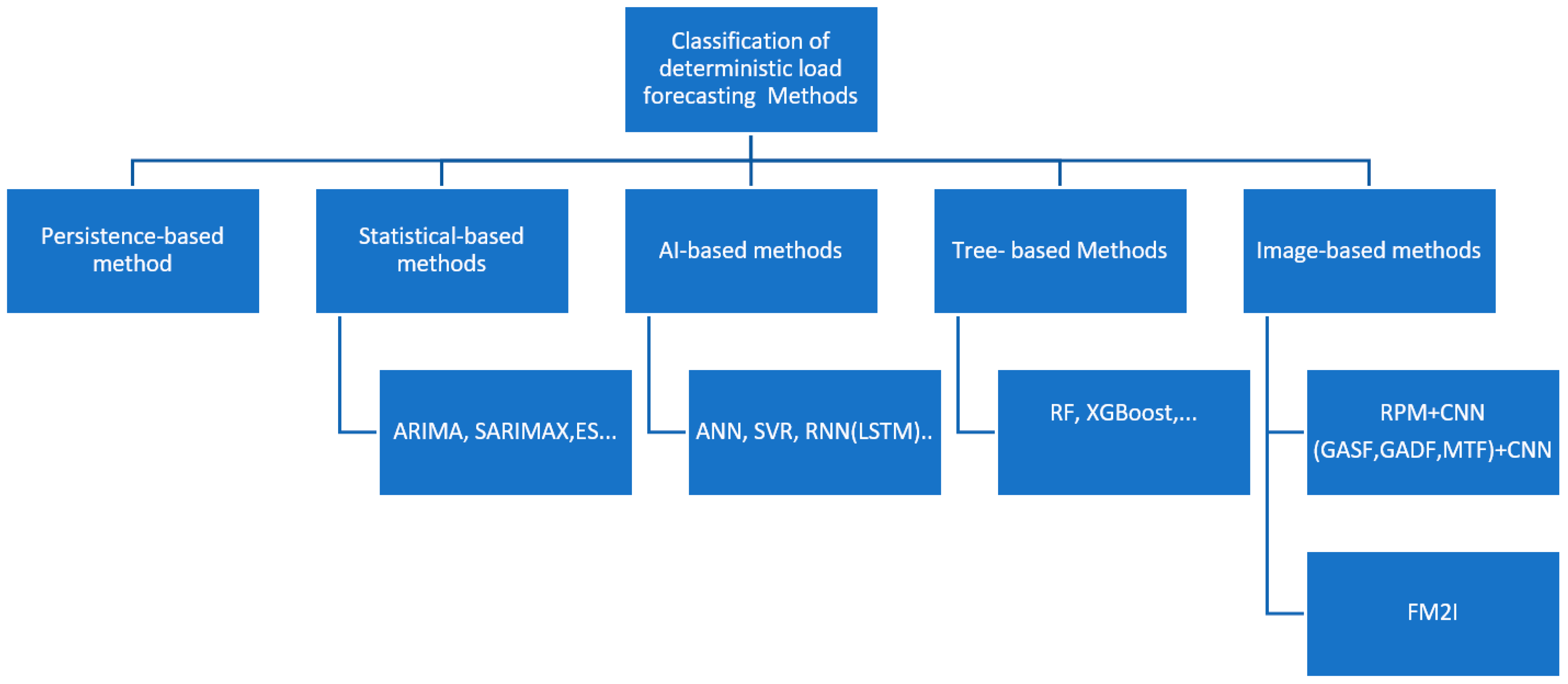
2. Forecasting Methods: An Overview

Over the last decades, a wide variety of deterministic methods for load forecasting has been proposed. We can classify them into five categories, as shown in Figure 1: persistence-based methods, statistical-based methods, artificial intelligence-based methods (AI), tree-based methods, and image-based methods.

Persistence-based or naïve forecasting methods are the simplest methods, which are used for producing forecasts. They are considered as a baseline or a reference in evaluating and comparing the accuracy of other models forecast. These naive forecasting methods predict the expected values for the next time step based on values of the previous time step. They are mainly based on the assumption that the forecasted conditions would not alter. These methods have the advantage of being easier to implement than other methods because they do not depend on weather forecast data or software toolkits for implementation. As a result, incorporating them into an embedded system is simple [27]. However, the persistent model’s accuracy degrades as forecasting time rises, and they do not account for any potential changes in electric power demand data related to external environmental factors.

Statistical-based methods include approaches based on mathematical equations. For instance, linear regression [28], the autoregressive integrated moving average (ARIMA), seasonal ARIMA [28], SARIMAX with exogenous variables and exponential smoothing (ES) techniques [29]. The use of those methods and their effectiveness primarily depend on the availability, quality and quantity of historical data, which are used as inputs. The key concept behind statistical-based methods is that they consider the used data linear by default. Otherwise, in satisfactory forecasting results may be obtained due to the non-linearity of the load data pattern [30].

However, if willing to consider the data as non-linear, artificial intelligence-based methods could be considered. These methods, such as neural network models, support vector regression (SVR) and fuzzy logic, are considered as data-driven approaches. In fact, these approaches utilize historical data learning process to capture even complex relations between inputs and futures outputs. Nevertheless, some of these techniques (e.g., Neural network models) suppose that no dependencies exist between the inputs and outputs, which is, in most cases, not true (e.g., sequential data) [31]. The AI based approaches also include a deep architecture neural network method, which is long short-term memory (LSTM). This method [32] has been proposed to solve the vanishing issues, and its effectiveness has been proved in diverse applications as well as in load forecasting field. LSTM model has been also used to tackle the multi-step ahead forecasting problem, as presented in [32], due to its ability to learn and to capture time series dependencies even for long-term horizon. Nevertheless, as presented in [33], LSTM has a significant computational time.

The fourth category groups tree-based methods, such as random forest, XGBOOST, classification and regression tree (CART), and LightGBM [34]. The tree-based methods are known not only for their remarkable performance in many machine-learning problems, but also for their ability to evaluate the features importance used in the forecasting process [35]. For instance, the XGBOOST model is an improvement of gradient boosted decision trees, which is basically developed by Chen and Guestrin [36,37] for both classification and regression. Its efficiency and accuracy in load forecasting exceed random forest, k-nearest neighbours (KNN), and SVM model, as stated in [38]. Nevertheless, tree-based methods are vulnerable to overfitting and underfitting, especially when dealing with limited datasets [39].

In recent research studies, an increasing interest in image-based approaches has been noticed. The image or graphical-based methods are presented in those studies according to two major strategies. The first one uses graphical-based methods for data preprocessing and then machine learning algorithm fore forecasting. For instance, Authors in [40], instead of depending on manual selection of the features, suggest first to encode the time series into images to automatically extract the features for being used in forecasting models; i. Similarly, three encoding methods (Gramian angular summation field (GASF), Gramian angular difference field (GADF), and Markov transition field (MTF)) were applied to convert a multivariate time series into a 2D image, which is used as an input to a convolutional neural network (ConvNet) [41]. The obtained results prove that these transformations have no effect in prediction results. The second strategy, presented in [42], relies completely on methods from image processing field, without resorting to other models for pre-processing and forecasting.

The work presented in this paper investigates three major algorithms from three categories, XGBOOST (tree-based), LSTM (AI based) and SARIMA (statistical based), for load forecasting. The aim is to evaluate them in order to figure out which one performs the best in forecasting electricity consumption, but with lower computational complexity. It is worth noting that other algorithms from image-based are under development and will be further considered in our ongoing work.

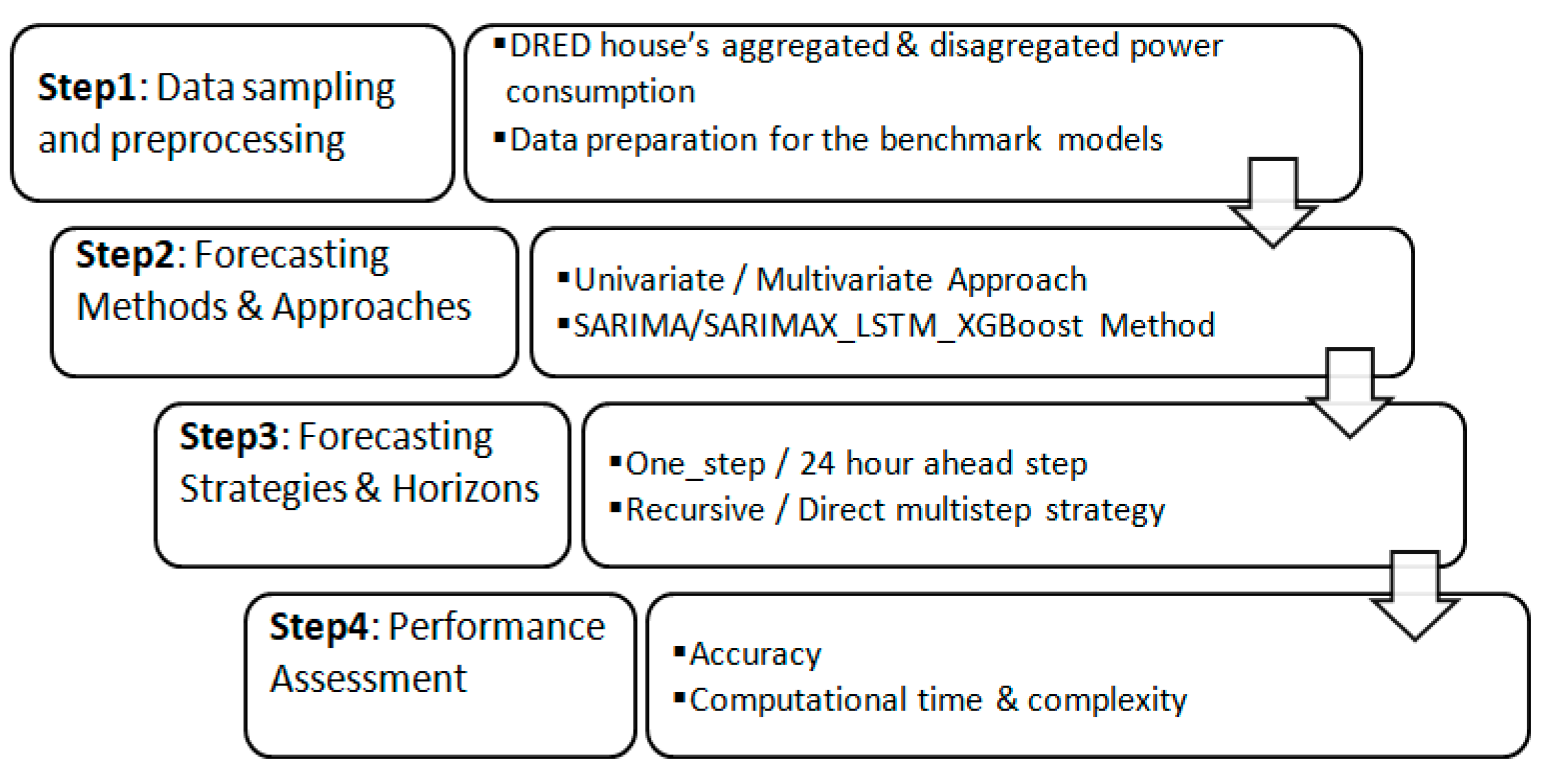
3. Materials and Methods

The procedure outlined in this paper, as presented in Figure 2, is structured into four main steps. The first step presents the dataset and tools we have applied for its preprocessing. The second step aims to explore forecasting approaches while using three different forecasting techniques. The forecasting horizons and strategies are developed in the third step. The last step addresses the performance evaluation by two key elements, precision or accuracy and computational time/complexity.

3.1. Power Consumption Dataset

Recently, several energy datasets have been publicly released as a result of non-intrusive load monitoring (NILM) research. In fact, these datasets provide fine-grained information about load consumption at aggregate level and household appliances level. Several characteristics differentiate these available datasets, such as the number of targeted houses, the number of installed sensors, the quality of the collected data, the measurement duration, and the sampling frequency.

The used dataset as a proof of concept for this comparative study is the Dutch Residential Energy Database (DRED) [43], which is publically available. This dataset contains several information, mainly aggregated and disaggregated electricity data, number of occupants, indoor temperature, and weather data. Actually, the dataset provides several information about electricity consumption at aggregate level and household appliances level (e.g., TV, fridges, washing machines, microwave, central heating, laptops). The available data of a single house were measured using smart plugs, which are installed in different locations in this house, and are collected for 12 successive days with a sampling frequency of 1 s.

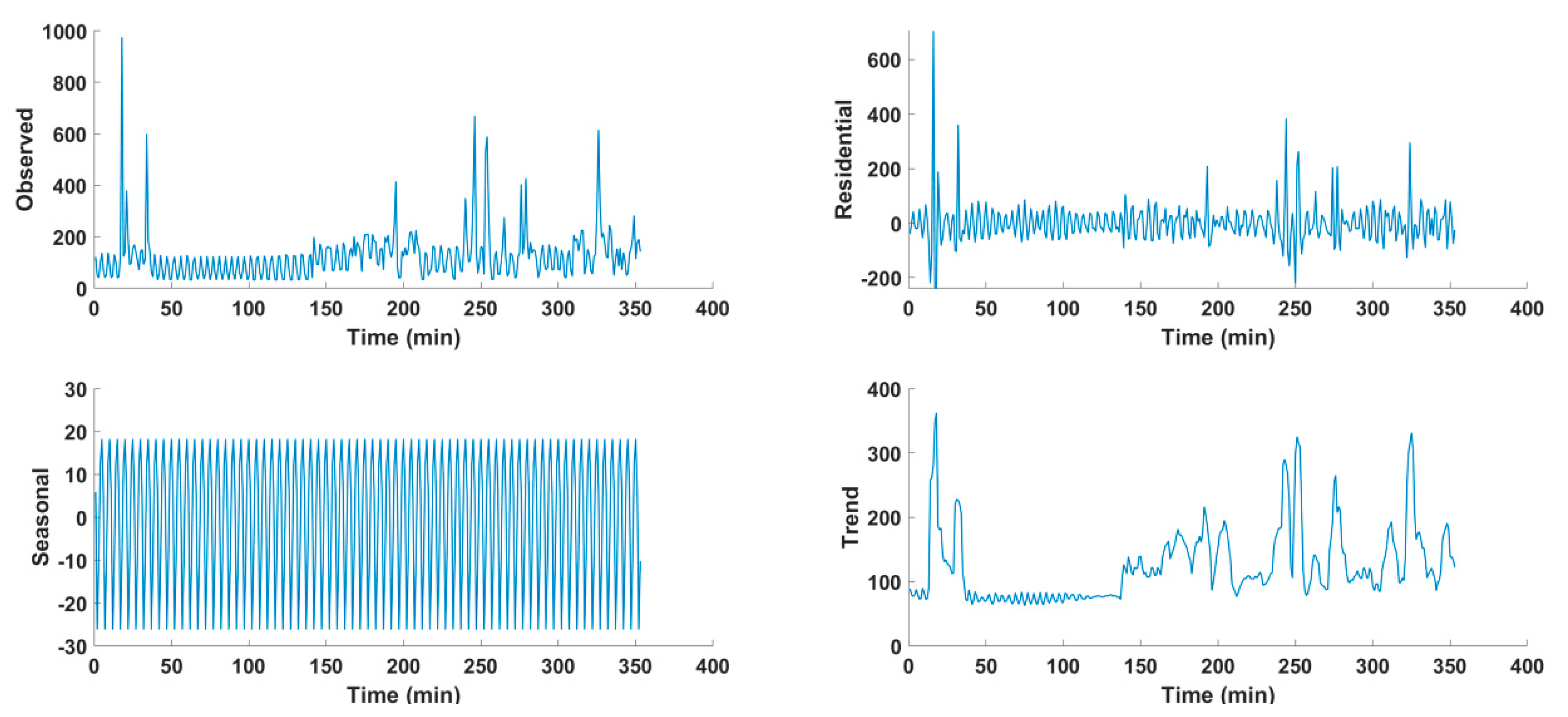
3.2. Dataset Sample Preprocessing and Feature Engineering

The preprocessing is one of the most common basics of time series analysis, presenting then good practices in machine learning [44]. This technique directly influences the quality of the forecast even if it consumes a significantly long period of time. In fact, the selected energy dataset does not need data cleaning methods since it has already been preprocessed. In this study, a data sample of five working days was extracted from DRED dataset, and then was re-sampled with a sampling frequency of 20 min in order to reduce the computational time, which is required to speed up the training process of used methods.

This data has been first analyzed using the exploratory data analysis functions. Among these functions, we have initially applied the summary statistics method, which includes eight statistical calculations of each variables (e.g., count, mean, standard deviation, minimum and maximum values, 25th, 50th and 75th percentiles), to the used data. Then, a graphical analysis tool, especially the histogram function, which provides a general insight into the shape of the consumption of each appliance, has been applied to this data. The additive decomposition tool, with the use of seasonal decompose function, has been afterwards applied in order to observe the seasonality, trends and randomness of the used dataset, as shown in Figure 3. It is to note that the values on the horizontal axis correspond to the time in minutes, starting from the 10th July 2015 at 01:00 AM, until the 14th July 2015 at 23:40 PM.

Secondly, we have used the augmented Dickey Fuller (ADF) function, which is a statistical test, in order to check the stationary of the used dataset. In fact, we have found that the p-values are less than 0.05. This proves that the used data is, indeed, stationary [45]. This allows us to say that data structure is time independent. Furthermore, the autocorrelation function (ACF) and the partial autocorrelation function (PACF), which are two methodical approaches used to interpret auto regressive (AR) and moving average (MA) terms for ARIMA or SARIMA models, were investigated. Thirdly, the normalization of the used data has been performed, so we can use the machine learning and tree-based methods. The normalization of the dataset has been performed by Min-Max Scaling function of scikit-learn library for the purpose of univariate and multivariate energy power forecasting. Then, the conversion of the normalized dataset into a supervised machine learning problem has been conducted. This conversion has been performed using the lag feature, which is a classical engineering procedure. Finally, a feature extraction method was used for the XGBOOST model in order to add time-based observations.

3.3. SARIMA, LSTM and XGBOOST

In this section, we provide a brief overview of the three considered methods. For instance, SARIMA is a statistical method, which relies on defining the SARIMA hyperparameters. These latter are tuned by the auto-arima function from the pmdarima statistical library. Using the stepwise model, it was deduced that the optimum selection for the SARIMA parameters is (0, 1, 2) (1, 1, 1)7.

The second experimented forecasting method was the LSTM. It is a particular version of recurrent neural network, which has a specific characteristic of taking into consideration the temporal correlations between past and present data. This ability is more convenient for forecasting household power consumption and it is modeled by setting up the look-back function. Our neural network architecture was developed using a sequential approach, with four neurons for the hidden layer and one neuron for the output layer. The model was trained for 100 epochs while using 1 for batch size. To obtain those optimal values, Hyperopt, a Python library, which implements a Bayesian optimization model to identify the best hyperparameters for a machine learning model, was employed. Also, our model was compiled by using the Adam algorithm [46], as a stochastic optimization technique.

The third experimented forecasting method is a highly performing implementation of gradient boosted trees, which is XGBOOST. This latter requires several hyperparameters while being constructed, since these parameters’ settings have a significant effect on its performance. An automated optimization technique was implemented to appropriately configure the parameter values. In fact, we have used the grid search method through GridSearchCV function, which determines the optimal parameters combination yielding, therefore, to more accurate results. It was noticed that the highest test score was reached when the number of decision trees defined by n-estimators is equal to 400, and the size of tree (max_depth parameter) is limited to six.

As for the second approach, instead of using only the aggregate energy data, twelve measurements of the household appliances were used to train the three models. Firstly, the seasonal ARIMA with exogenous regressors model was developed to deal with that multivariate time series. To serve this purpose, the consumption of 12 household appliances was integrated, after proving their stationarity. In order to investigate the best parameters for the seasonal ARIMAX models, a grid search was performed based on the lowest result of the Akaike information criterion (AIC).

Regarding the LSTM model, a transformation into a supervised machine learning problem was needed before developing the RNN model for the multivariate approach. This first data modeling was involved to predict the total power consumption at time (t + 1) based on the energy consumed by household appliances for the prior time (t). Actually, 80% of the used dataset were taken as a training set and split into inputs and outputs. As for the other 20%, they were used as testing set and were also split in the same way.

In response to the LSTM typical format requirement [32], input data were converted into 3D shape. For this, three main parameters are to be defined, starting with the number of features, which was given as 13. Besides, the time step was configured to 1 as a way to determine the number of loop layers in our model.

The last algorithm of the second approach, which is the XGBOOST model, was applied to process with multivariate inputs problem. Actually, the column, which contains the house’s aggregated power consumption, was used as the target column and the 12 household’s appliances were included as features columns. As in the previous approach, the same strategy setting has been applied to tune XGBOOST hyper-parameters. The optimal configuration for the multivariate case was a value of 150 for the n_estimators parameter, a maximum depth of 8 with a default setting for the max_features. A feature importance method was used in order to depict the usefulness of each feature during the construction of our model according to their importance score.

The proposed study includes the third approach to forecast the DRED house’s aggregated power consumption for multiple time-steps ahead. In fact, we chose to forecast the power consumption for a period of 24 h with a sampling frequency of one hour instead of 20 min. Although, this kind of forecast is highly requested in several research areas, only few works discuss it in literature [47]. According to the literature reviews, four procedures have been proposed to figure out multistep forecasting scenarios. Starting by the recursive strategy, it is considered to be one of the oldest multi-step forecast strategy since it involves the use of a single model for different forecast horizons, while significantly reducing computational time. Nevertheless, this strategy appears to be less effective if we raise the forecast horizon, and this is due to accumulated prediction errors, which is associated to this increase [48]. The second strategy is the direct one, which consists of constructing different models, one model for each forecast horizon, instead of having a single model. More specifically, forecasting desired and future time intervals of the house’s power consumption with different trained models. However, since the training was carried out separately, this strategy may not guarantee any conditional dependency between predicted values.

Another strategy, which seems to combine the efficiency of both above discussed strategies, according to [49], is the DirRec strategy. This latter is based on the development of different models for each forecast horizon (similar to direct strategy), but with the condition that each model takes into consideration the prediction obtained at the prior period as inputs for the following model.

The fourth one is the multiple-output strategy, which aims to surmount the constraints related to the direct strategy [50]. This can be done thanks to two sub strategies, notably MIMO (multiple-input multiple-output) and MISMO, which adds the optimal S criterion. This latter defines the size of the outputs (forecast horizons) [51]. In the same work, authors propose a specific way of solving the problem of conditional independence by replacing different independent training models with one model capable of predicting several outputs at once.

4. Results and Discussion

This section presents the results obtained for the three discussed approaches using three representative methods, SARIMA, LSTM and XGBOOST. In order to provide sufficient empirical evidence for the performance of each aforementioned approach, multiple error metrics are implemented as performance indicators. In fact, to assess the accuracy of the various methods, a set of six popular performance metrics (the mean percentage error (MPE), the mean absolute percentage error (MAPE), the mean absolute error (MAE), root mean squared Error (RMSE), the symmetric mean absolute percentage error (sMAPE), and the mean absolute scaled error (MASE) [52]) have been also calculated. For comparison reliability purposes, all the chosen developed forecasting models thereafter have been using the same training and testing sets.

In addition, the performance of the abovementioned methods is also evaluated by the computational complexity (CC). This latter can be calculated by dividing the computational time necessary to accomplish the forecast by the relative time necessary for a naïve method (e.g., ARIMA). It is worth noting that the system characteristics used to approximate the computational time are an Intel^® Core™ i5-5300U CPU @ 2, 30 GHz, 16.00 GB RAM, x64-based processor.

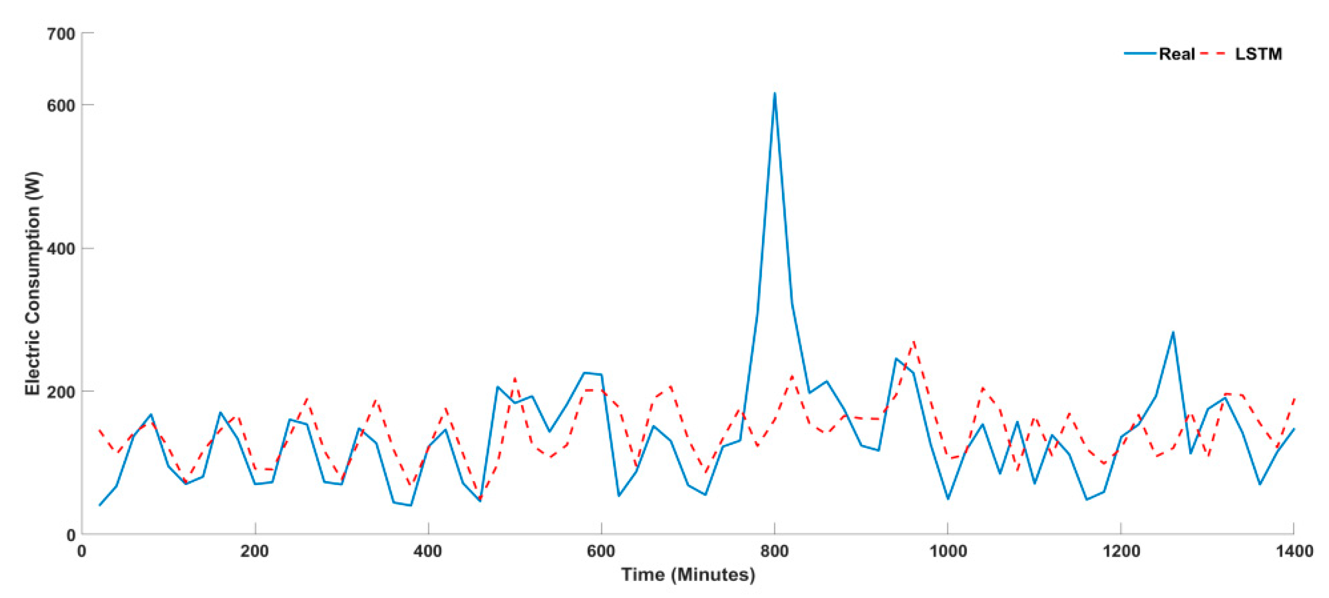
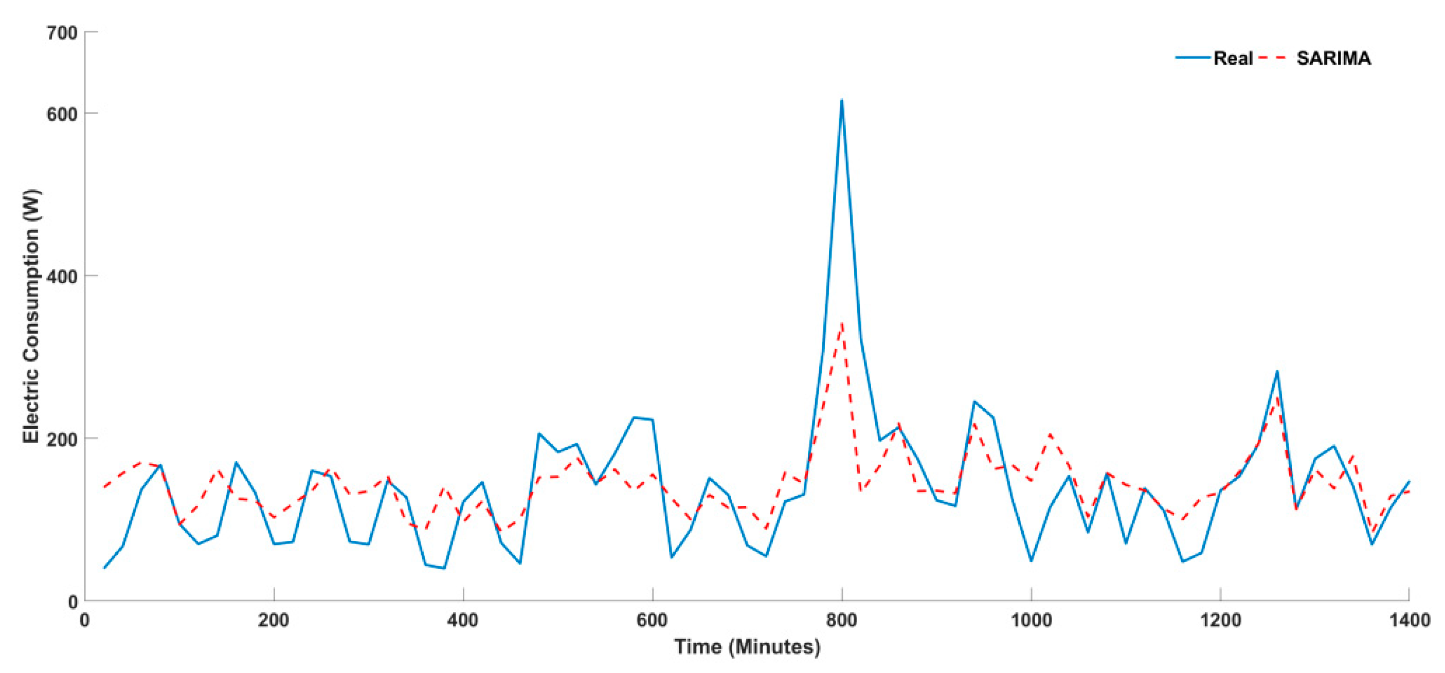
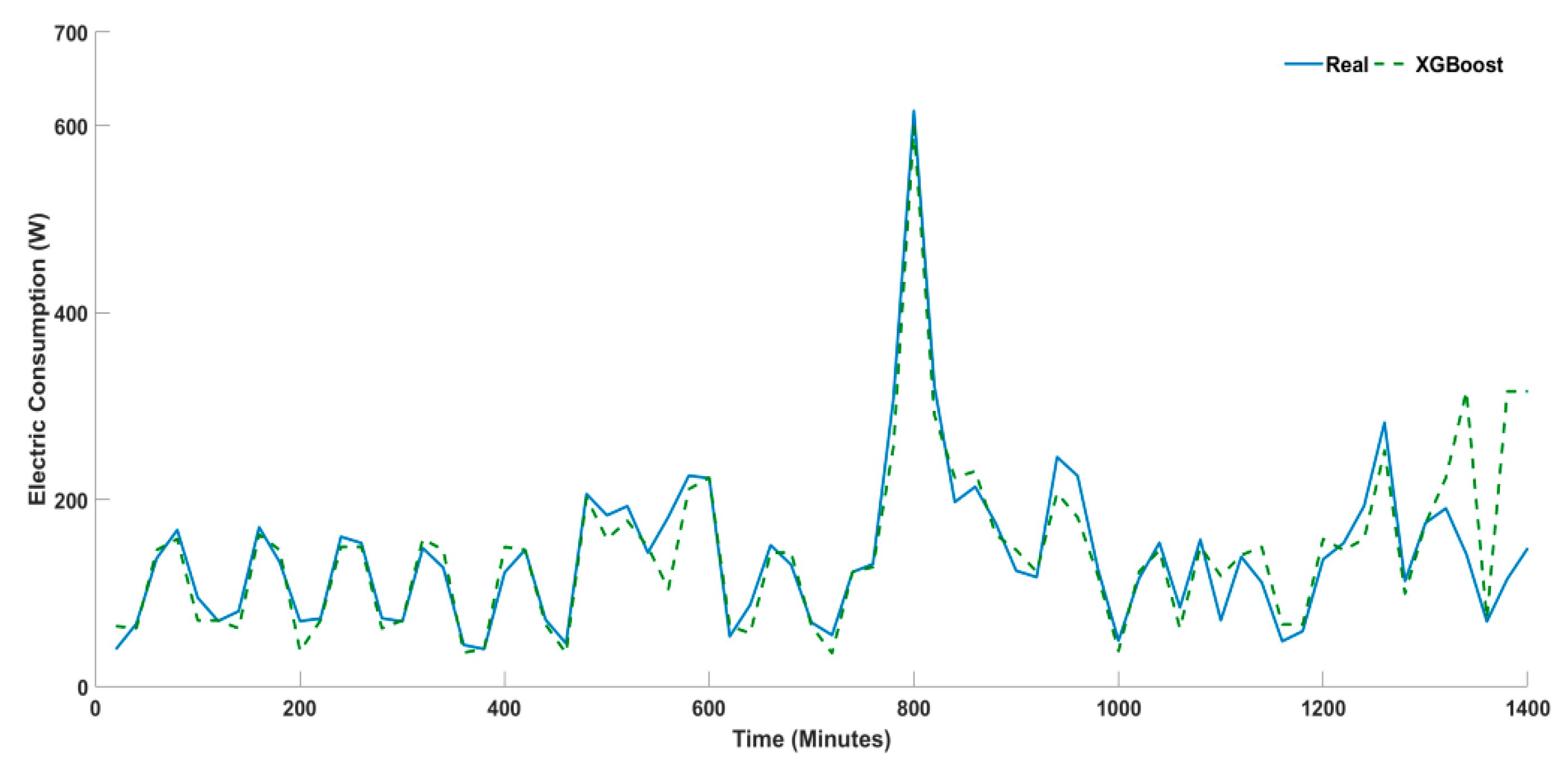
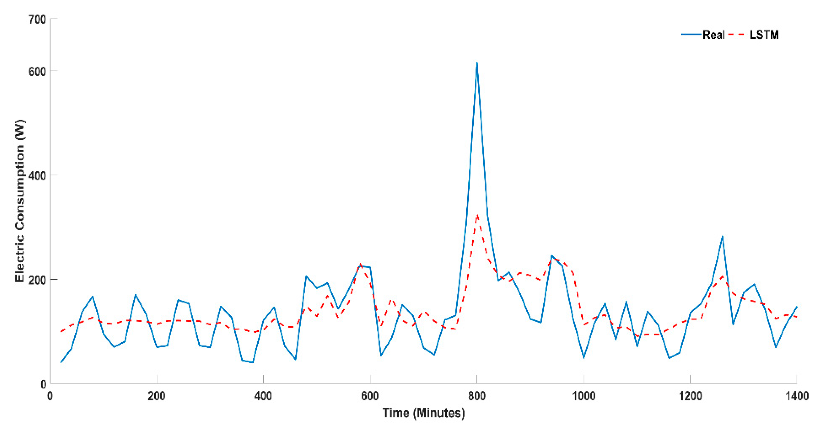
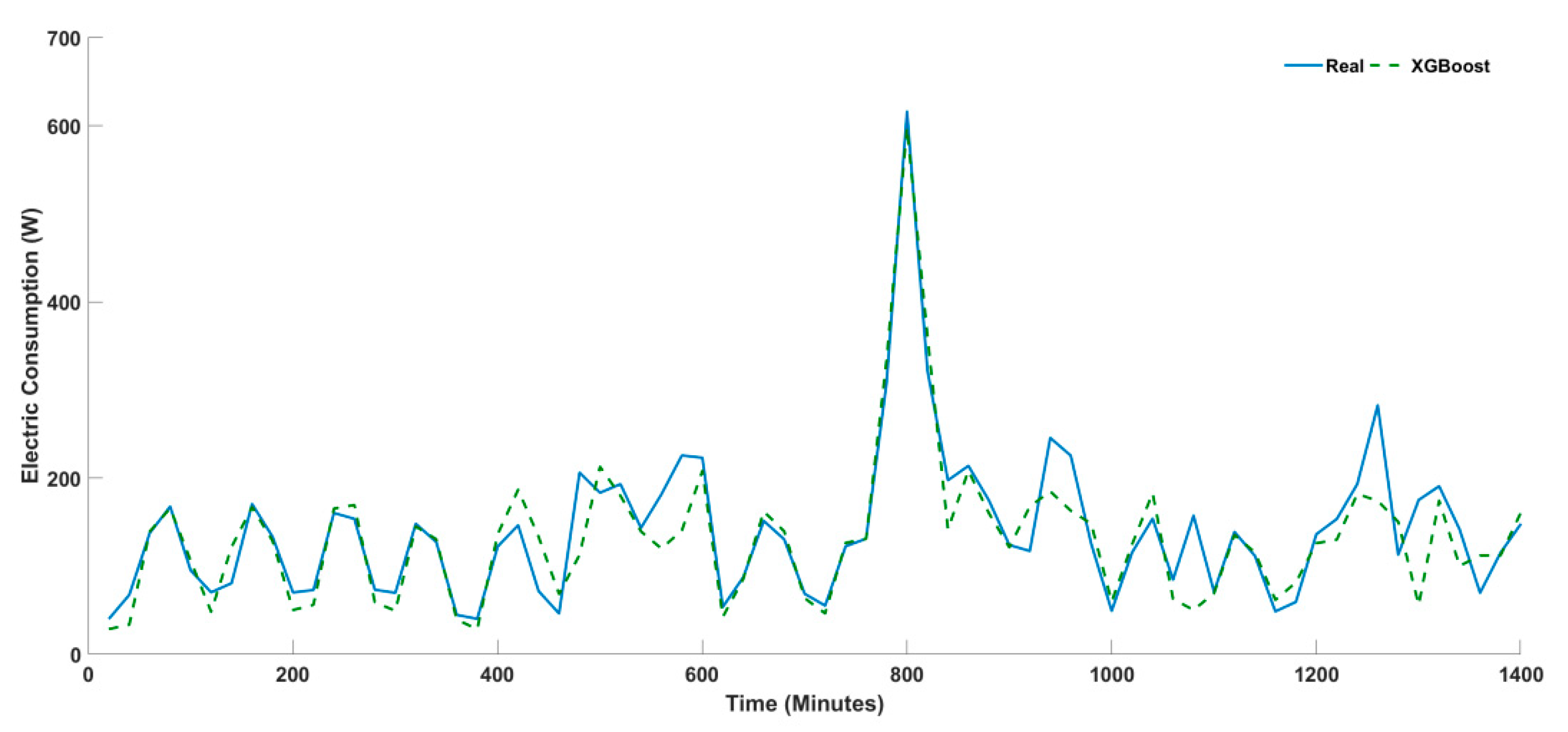
4.1. Univariate Timeseries Forecasting

In the first experiment, we predict the house’s aggregated power consumption using only the historical data. More specifically, only one day ahead for aggregated power consumption has been predicted, which we consider as univariate short term load forecasting. However, the number of predicted values for a day will be equal to 72; since as described before, the dataset was sampled to 20 min.

Figure 4, Figure 5 and Figure 6 present the results obtained for the used forecasting methods in comparison to the test set. In fact, we can notice that SARIMA and LSTM methods are outperformed by the XGBOOST method.

Table 2. Results & ranking of the performance metrics.

Method	RMSE	MAE	MAPE	MPE	sMAPE	MASE	Ranking
							RMSE	MAE	MAPE	MPE	sMAPE	MASE
LSTM	35.412	10.304	8.930	5.146	36.712	0.852	3	3	3	3	3	3
SARIMA	26.375	7.988	8.319	−5.355	31.075	0.656	2	2	2	1	2	2
XGBOOST	19.030	4.495	3.716	−0.789	16.886	0.372	1	1	1	2	1	1

proves this interpretation, as it can be observed the XGBOOST has the lowest results in terms of all error measurements. Actually, the XGBOOST model has the ability to deal with non-linear patterns and yields significant results. Furthermore, the findings presented in [53] confirm the effectiveness of the XGBOOST model, since it has achieved the lowest prediction errors when compared to ARIMA. It is worth noting that the objective of this study was to anticipate electric energy usage in non-residential buildings.

The performance of the LSTM model, for univariate energy data, was also evaluated in [54], which employed a different publicly available dataset (UK-DALE). When compared to the LSTM results, which were obtained for the DRED dataset, the findings of this comparative study done on a resolution of 20 min had slightly higher error rates.

We can also note, from the obtained results, that for all the three forecasting methods, the MASE values are less than one, which confirms that all the used methods are more efficient than just a naïve forecasting method [55].

Table 3. Computational complexity for univariate time series.

Method	Computational Time (s)	CC
SARIMA	5.85	83.58
LSTM	2.85	40.72
XGBOOST	0.12	1.72

gives an overview of the computational time and complexity of applied methods, those information are essential for future implementation in an embedded system (i.e., smart meter having predictive capabilities). As expected, the shortest processing time is achieved by the XGBOOST method, which is known for its efficiency.

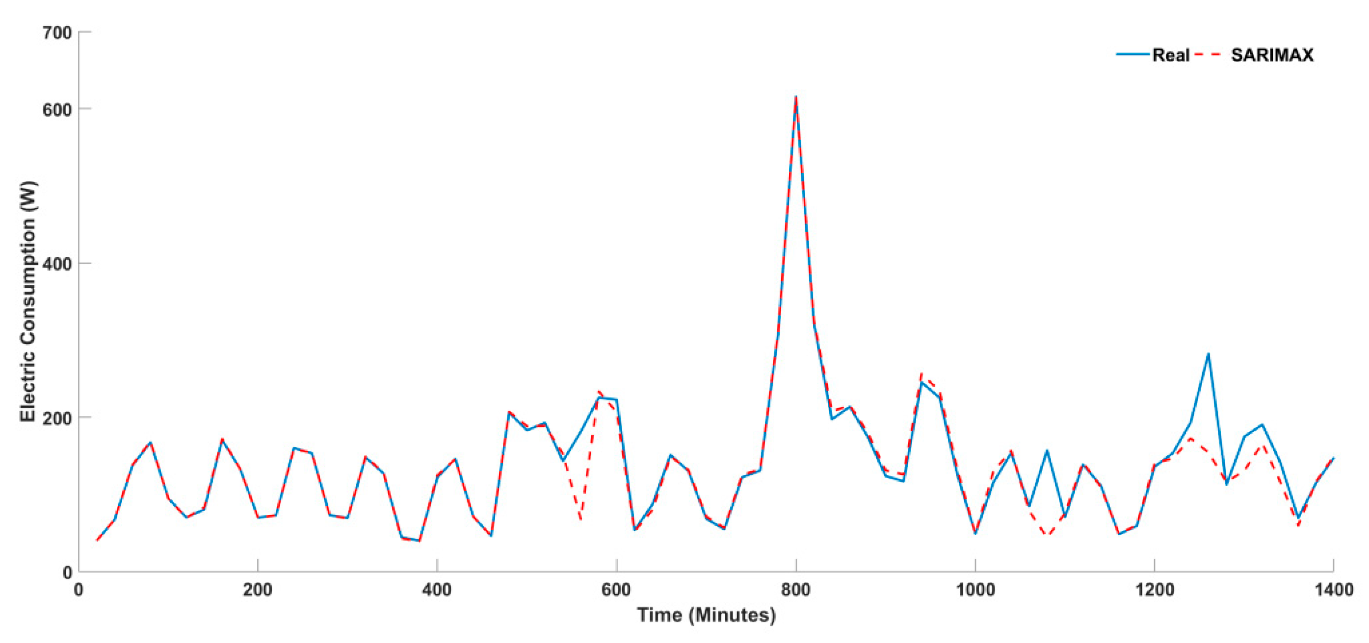
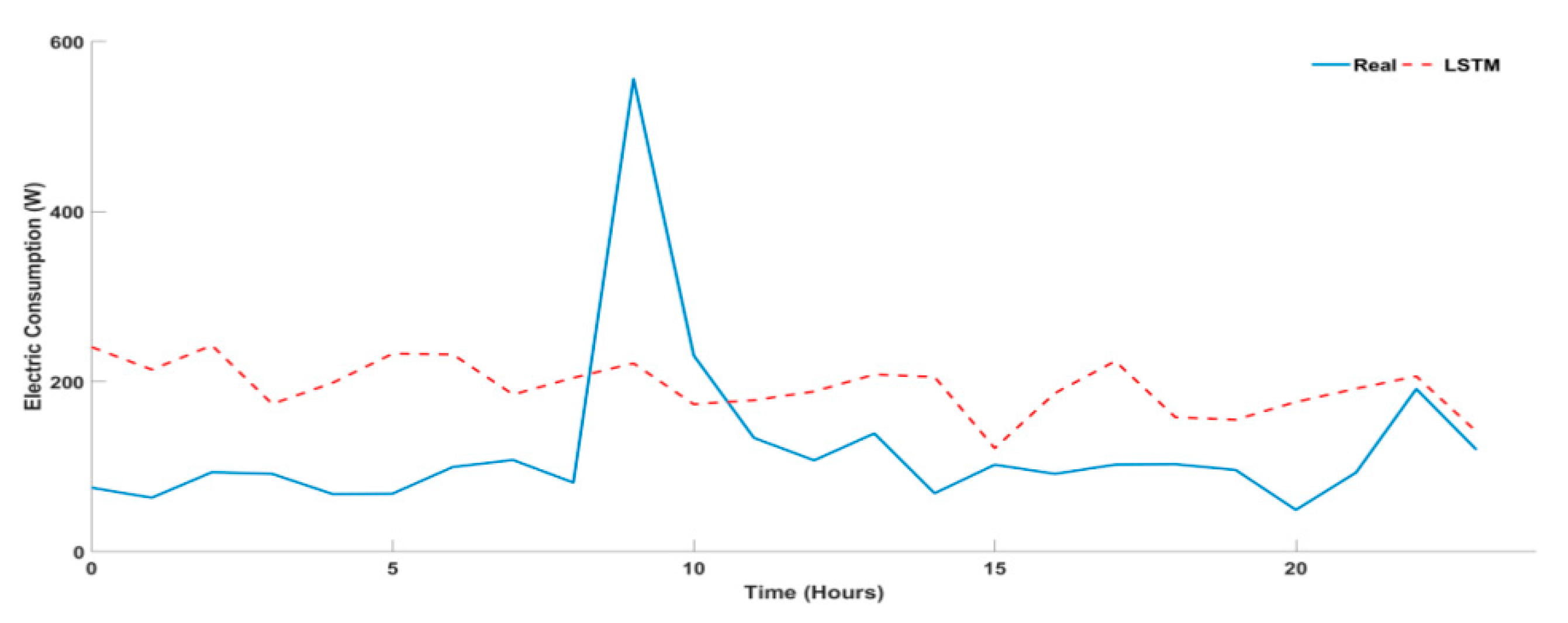
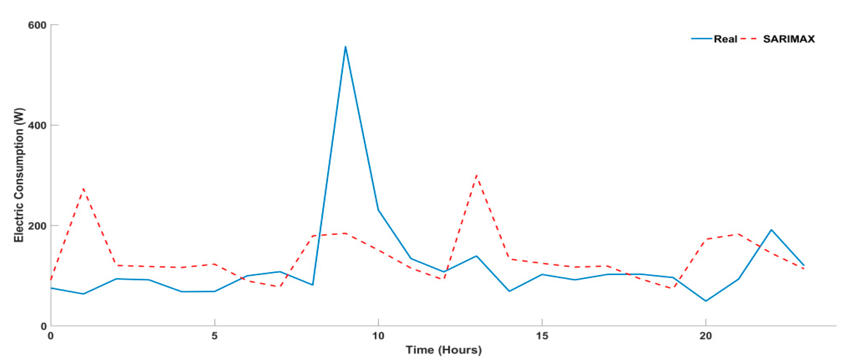
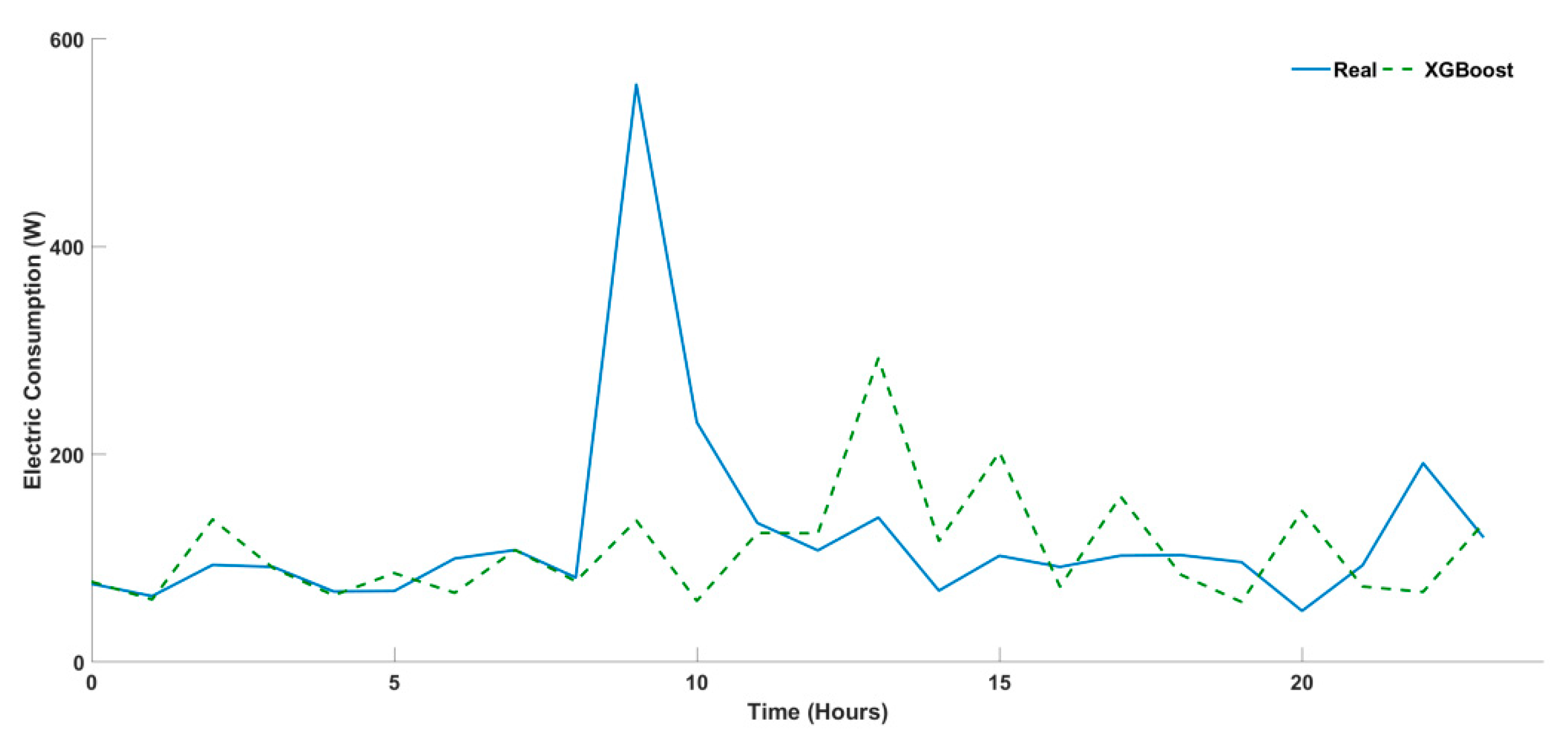
4.2. Multivariate Timeseries Forecasting

In this section, the effect of the second method is investigated. It consists of forecasting the overall power consumption of the house, using the disaggregated power consumption of the appliances. Our analysis has been performed as a multivariate forecasting process using twelve features in order to determine their effects on the forecast accuracy.

Figure 7, Figure 8 and Figure 9 show the forecast results obtained for the multivariate method. It can be seen that the forecast results for the multivariate method are on average more accurate than the univariate one. In fact, adding the power consumption of each appliance as exogenous variables has a positive effect on the results of all models, as shown in

Table 4. Results & ranking of the performance metrics.

Method	RMSE	MAE	MAPE	MPE	sMAPE	MASE	Ranking
							RMSE	MAE	MAPE	MPE	sMAPE	MASE
LSTM	25.296	8.365	8.268	−4.448	33.610	0.692	3	3	3	1	3	3
XGBOOST	16.332	4.918	3.952	0.687	21.266	0.402	2	2	2	3	2	2
SARIMAX	11.471	1.905	1.162	0.544	7.217	0.157	1	1	1	2	1	1

. According to the performance metrics presented in Table 4, the SARIMA with exogenous variable (SARIMAX) method yields lower error results compared to its competitor methods.

These interpretations can be backed up by the research work presented in [56]. Introducing appliance measurement into the training dataset enhances the forecast performance for LSTM. However, if we consider these measures as exogenous variables in the SARIMAX process, a greater performance improvement can be observed.

Table 5. Computational complexity for multivariate time series.

Method	Computational Time (s)	CC
SARIMAX	11.83	131.45
LSTM	3.36	37.34
XGBOOST	0.24	2.67

depicts the computational complexity for the three models. The lowest CC value is assigned to XGBOOST.

4.3. Univariate Time Series for Multi-Step Approach

In order to investigate the multi-step ahead forecasting approach, we used similar methods with different frequency samples as shown in Figure 10, Figure 11 and Figure 12. More precisely, an hourly frequency sampling is used as a solution for computation time issue. In fact, two multi-step forecasting strategies are deployed, in particular the recursive and the direct. We opted for the SARIMAX and LSTM as recursive strategies and the XGBOOST as a direct one. A model is built to be used iteratively in LSTM and SARIMAX methods in order to forecast a day ahead of load consumption. As for the XGBOOST method, a separate forecasting model is developed, for each time step during the 24 h.

The sMAPE metric actually indicates that the lowest score is assigned to the XGBOOST method, based on the results provided in

Table 6. Results & ranking of the performance metrics.

Method	RMSE	MAE	MAPE	MPE	sMAPE	MASE	Ranking
							RMSE	MAE	MAPE	MPE	sMAPE	MASE
LSTM	50.453	17.439	18.635	17.454	65.925	1.623	3	3	3	3	3	3
XGBOOST	43.787	9.827	6.964	−1.789	39.028	0.915	2	1	1	1	1	1
SARIMAX	42.826	11.066	10.638	7.427	43.211	1.029	1	2	2	2	2	2

. Consequently, the XGBOOST outperforms other techniques for multi-step forecasting.

These unexpected results from robust models like LSTM method might be caused by the small size of the sample dataset. According to [57], machine learning methods are less efficient when dealing with a small dataset.

Table 7. Results Computational complexity for multistep ahead forecasting.

Method	Computational Time (s)	CC
SARIMAX	14.05	8.363
LSTM	23.36	13.904
XGBOOST (Recursive)	2.67	1.589
XGBOOST(With hyperparameter optimization function)	52.03	30.970
XGBOOST(Direct)	612.63	364.661

gives the computational time and complexity for 24 h ahead forecasting, three results are presented for XGBOOST model. The first one for the recursive strategy with a single training, the second results with the addition of hyperparameters optimization function and the last one represents the time necessary to perform the direct multi-step forecast.

Table 8. Computational complexity and sMAPE for multistep ahead forecasting.

Forecast Horizon (H)	Computational Time for XGBOOST (Direct Strategy) (s)	CC	sMAPE (%)
4 steps	110.46	65.75	39.53
8 steps	234.95	139.85	33.11
12 steps	325.09	193.51	40.07
16 steps	401.58	239.04	38.35
20 steps	512.03	304.78	45.58
24 steps	612.63	364.67	39.03

presents an assessment of the computational complexity of the direct multi-step forecast for each horizon though MAPE. A similarity of the sMAPE results obtained can be observed even though the direct strategy has the ability to train the model for each time step. In practice, to achieve real-time forecasting, the best strategy for embedded systems is to find a trade-off between efficiency and performance.

5. Conclusions and Perspectives

In this paper, we have investigated three major approaches for electricity consumption forecasting in buildings. For this matter, we putted more emphasize on three main strategies, univariate, multivariate for 1-step ahead and univariate for n-step-ahead. We have selected three main representatives forecasting methods (SARIMA, LSTM, XGBOOST) accordingly and compared them in terms of computational time/complexity and accuracy. In fact, extensive experiments have been conducted using a public dataset, which includes sensors data, such as weather, occupancy, and disaggregated power consumption. Obtained results showed that none of them outperforms efficiently in the three forecasting strategies (i.e., univariate, multivariate and multistep). For instance, XGBOOST outperforms well for univariate and multistep forecasting against ARIMA variants, which showed better performance for multivariate. However, LSTM showed the worst behavior in the three strategies. As a perspective, since the XGBOOST showed the better tradeoff in terms of accuracy and CC, it will be deployed in our IoT platform for real-time electricity consumption forecasting. More experiments will be conducted on real-sitting scenarios when implemented in our embedded metering platform.

References

1. Iwafune, Y.; Yagita, Y.; Ikegami, T.; Ogimoto, K. Short-term forecasting of residential building load for distributed energy management. In Proceedings of the 2014 IEEE International Energy Conference (ENERGYCON), Cavtat, Croatia, 13–16 May 2014; pp. 1197–1204. [Google Scholar]
2. Gajowniczek, K.; Za̧bkowski, T.; Szupiluk, R. Blind Source Separation for Improved Load Forecasting on Individual Household Level. Adv. Intell. Syst. Comput. 2016, 403, 181–190. [Google Scholar]
3. Malekizadeh, M.; Karami, H.; Karimi, M.; Moshari, A.; Sanjari, M.J. Short-term load forecast using ensemble neuro-fuzzy model. Energy 2020, 196, 117127. [Google Scholar] [CrossRef]
4. Lusis, P.; Khalilpour, R.; Andrew, L.; Liebman, A. Short-term residential load forecasting: Impact of calendar effects and forecast granularity. Appl. Energy 2017, 205, 654–669. [Google Scholar] [CrossRef]
5. Dumas, J.; Cornélusse, B. Classification of load forecasting studies by forecasting problem to select load forecasting techniques and methodologies. arXiv 2018, arXiv:1901.05052. [Google Scholar]
6. Hong, T.; Fan, S. Probabilistic electric load forecasting: A tutorial review. Int. J. Forecast. 2016, 32, 914–938. [Google Scholar] [CrossRef]
7. Haq, I.; Ullah, A.; Khan, S.; Khan, N.; Lee, M.; Rho, S.; Baik, S. Sequential Learning-Based Energy Consumption Prediction Model for Residential and Commercial Sectors. Mathematics 2021, 9, 605. [Google Scholar] [CrossRef]
8. Chakhchoukh, Y.; Panciatici, P.; Mili, L. Electric Load Forecasting Based on Statistical Robust Methods. IEEE Trans. Power Syst. 2011, 26, 982–991. [Google Scholar] [CrossRef]
9. Yuce, B.; Mourshed, M.; Rezgui, Y. A Smart Forecasting Approach to District Energy Management. Energies 2017, 10, 1073. [Google Scholar] [CrossRef] [Green Version]
10. Ahmed, A.; Khalid, M. Multi-step Ahead Wind Forecasting Using Nonlinear Autoregressive Neural Networks. Energy Procedia 2017, 134, 192–204. [Google Scholar] [CrossRef]
11. Majidpour, M.; Nazaripouya, H.; Chu, P.; Pota, H.R.; Gadh, R. Fast Univariate Time Series Prediction of Solar Power for Real-Time Control of Energy Storage System. Forecasting 2018, 1, 107–120. [Google Scholar] [CrossRef] [Green Version]
12. Elmouatamid, A.; NaitMalek, Y.; Bakhouya, M.; Ouladsine, R.; Elkamoun, N.; Zine-Dine, K.; Khaidar, M. An energy management platform for micro-grid systems using Internet of Things and Big-data technologies. Proc. Inst. Mech. Eng. Part I J. Syst. Control. Eng. 2019, 233, 904–917. [Google Scholar] [CrossRef]
13. Cai, M.; Pipattanasomporn, M.; Rahman, S. Day-ahead building-level load forecasts using deep learning vs. traditional time-series techniques. Appl. Energy 2019, 236, 1078–1088. [Google Scholar] [CrossRef]
14. Mtibaa, F.; Nguyen, K.-K.; Azam, M.; Papachristou, A.; Venne, J.-S.; Cheriet, M. LSTM-based indoor air temperature prediction framework for HVAC systems in smart buildings. Neural Comput. Appl. 2020, 32, 1–17. [Google Scholar] [CrossRef]
15. Xue, P.; Jiang, Y.; Zhou, Z.; Chen, X.; Fang, X.; Liu, J. Multi-step ahead forecasting of heat load in district heating systems using machine learning algorithms. Energy 2019, 188, 116085. [Google Scholar] [CrossRef]
16. Abdel-Aal, R. Univariate modeling and forecasting of monthly energy demand time series using abductive and neural networks. Comput. Ind. Eng. 2008, 54, 903–917. [Google Scholar] [CrossRef]
17. Chaouch, M. Clustering-Based Improvement of Nonparametric Functional Time Series Forecasting: Application to Intra-Day Household-Level Load Curves. IEEE Trans. Smart Grid 2014, 5, 411–419. [Google Scholar] [CrossRef]
18. Ghofrani, M.; Hassanzadeh, M.; Etezadi-Amoli, M.; Fadali, M.S. Smart meter based short-term load forecasting for residential customers. In Proceedings of the North American Power Symposium, Boston, MA, USA, 4–6 August 2011; pp. 1–5. [Google Scholar] [CrossRef]
19. Teeraratkul, T.; O’Neill, D.; Lall, S. Shape-Based Approach to Household Electric Load Curve Clustering and Prediction. IEEE Trans. Smart Grid 2018, 9, 5196–5206. [Google Scholar] [CrossRef]
20. Haben, S.; Ward, J.; Greetham, D.V.; Singleton, C.; Grindrod, P. A new error measure for forecasts of household-level, high resolution electrical energy consumption. Int. J. Forecast. 2014, 30, 246–256. [Google Scholar] [CrossRef] [Green Version]
21. Quilumba, F.; Lee, W.-J.; Huang, H.; Wang, D.Y.; Szabados, R.L. Using Smart Meter Data to Improve the Accuracy of Intraday Load Forecasting Considering Customer Behavior Similarities. IEEE Trans. Smart Grid 2015, 6, 911–918. [Google Scholar] [CrossRef]
22. Da Silva, P.G.; Ilic, D.; Karnouskos, S. The Impact of Smart Grid Prosumer Grouping on Forecasting Accuracy and Its Benefits for Local Electricity Market Trading. IEEE Trans. Smart Grid 2013, 5, 402–410. [Google Scholar] [CrossRef]
23. Chen, Y.; Luh, P.B.; Guan, C.; Zhao, Y.; Michel, L.D.; Coolbeth, M.A.; Friedland, P.B.; Rourke, S.J. Short-Term Load Forecasting: Similar Day-Based Wavelet Neural Networks. IEEE Trans. Power Syst. 2010, 25, 322–330. [Google Scholar] [CrossRef]
24. Alotaibi, R.; Jin, N.; Wilcox, T.; Flach, P. Feature Construction and Calibration for Clustering Daily Load Curves from Smart-Meter Data. IEEE Trans. Ind. Inform. 2016, 12, 645–654. [Google Scholar] [CrossRef] [Green Version]
25. Basu, K.; Hawarah, L.; Arghira, N.; Joumaa, H.; Ploix, S. A prediction system for home appliance usage. Energy Build. 2013, 67, 668–679. [Google Scholar] [CrossRef]
26. Dinesh, C.; Makonin, S.; Bajic, I.V. Residential Power Forecasting Using Load Identification and Graph Spectral Clustering. IEEE Trans. Circuits Syst. II Express Briefs 2019, 66, 1900–1904. [Google Scholar] [CrossRef]
27. Dutta, S.; Li, Y.; Venkataraman, A.; Costa, L.M.; Jiang, T.; Plana, R.; Tordjman, P.; Choo, F.H.; Foo, C.F.; Puttgen, H.B. Load and Renewable Energy Forecasting for a Microgrid using Persistence Technique. Energy Procedia 2017, 143, 617–622. [Google Scholar] [CrossRef]
28. Hinman, J.; Hickey, E. Modeling and Forecasting Short-Term Electricity Load Using Regression Analysis; Illinois State University: Normal, IL, USA, 2009; pp. 1–51. [Google Scholar]
29. Christiaanse, W.R. Short-Term Load Forecasting Using General Exponential Smoothing. IEEE Trans. Power Appar. Syst. 1971, 90, 900–911. [Google Scholar] [CrossRef]
30. Chan, S.-C.; Tsui, K.M.; Wu, H.C.; Hou, Y.; Wu, Y.C.; Wu, F.F. Load/Price Forecasting and Managing Demand Response for Smart Grids: Methodologies and Challenges. IEEE Signal Process. Mag. 2012, 29, 68–85. [Google Scholar] [CrossRef]
31. Khashei, M.; Bijari, M. An artificial neural network (p,d,q) model for timeseries forecasting. Expert Syst. Appl. 2010, 37, 479–489. [Google Scholar] [CrossRef]
32. Yunpeng, L.; Hou, D.; Junpeng, B.; Yong, Q. Multi-step Ahead Time Series Forecasting for Different Data Patterns Based on LSTM Recurrent Neural Network. In Proceedings of the 2017 14th Web Information Systems and Applications Conference (WISA), Liuzhou, China, 11–12 November 2017; pp. 305–310. [Google Scholar] [CrossRef]
33. Bouktif, S.; Fiaz, A.; Ouni, A.; Serhani, M.A. Optimal Deep Learning LSTM Model for Electric Load Forecasting using Feature Selection and Genetic Algorithm: Comparison with Machine Learning Approaches. Energies 2018, 11, 1636. [Google Scholar] [CrossRef] [Green Version]
34. Guolin, K.; Qi, M.; Thomas, F.; Taifeng, W.; Wei, C.; Weidong, M.; Qiwei, Y.; Tie-Yan, L. LightGBM: A Highly Efficient Gradient Boosting Decision Tree. Adv. Neural Inf. Process. Syst. 2017, 30, 3146–3154. [Google Scholar]
35. Papadopoulos, S.; Azar, E.; Woon, W.L.; Kontokosta, C. Evaluation of tree-based ensemble learning algorithms for building energy performance estimation. J. Build. Perform. Simul. 2017, 11, 322–332. [Google Scholar] [CrossRef]
36. Chen, T.; Guestrin, C. XGBoost: A Scalable Tree Boosting System. In Proceedings of the 22nd ACM SIGKDD International Conference on Knowledge Discovery Data Mining KDD ’16, San Francisco, CA, USA, 13–17 August 2016; pp. 785–794. [Google Scholar] [CrossRef] [Green Version]
37. Friedman, J.H. Stochastic gradient boosting. Comput. Stat. Data Anal. 2002, 38, 367–378. [Google Scholar] [CrossRef]
38. Li, G.; Wenjia, L.; Tian, X.; Yifeng, C. Short-Term Electricity Load Forecasting Based on the XGBOOST Algorithm. Smart Grid 2017, 7, 274–285. [Google Scholar] [CrossRef]
39. Song, Y.-Y.; Lu, Y. Decision tree methods: Applications for classification and prediction. Shanghai Arch Psychiatry 2015, 27, 130–135. [Google Scholar] [CrossRef] [PubMed]
40. Li, X.; Kang, Y.; Li, F. Forecasting with time series imaging. Expert Syst. Appl. 2020, 160, 113680. [Google Scholar] [CrossRef]
41. Yang, C.-L.; Zhi-Xuan, C.; Chen-Yi, Y. Sensor Classification Using Convolutional Neural Network by En-coding Multivariate Time Series as Two-Dimensional Colored Images. Sensors 2020, 20, 168. [Google Scholar] [CrossRef] [Green Version]
42. Maaroufi, N.; Mehdi, N.; Mohamed, B. Predicting the Future is like Completing a Painting! arXiv 2020, arXiv:2011.04750. [Google Scholar]
43. Nambi, A.S.N.U.; Lua, A.R.; Prasad, V.R. LocED: Location-aware Energy Dis-aggregation Framework. In Proceedings of the 2nd ACM International Conference on Embedded Systems for Energy-Efficient Built Environments (BuildSys’15), Seoul, Korea, 4–5 November 2015; Association for Computing Machinery: New York, NY, USA, 2019; pp. 45–54. [Google Scholar]
44. Kotsiantis, S.; Kanellopoulos, D.; Pintelas, P. Data Preprocessing for Supervised Learning. Int. J. Comput. Sci. 2006, 1, 111–117. [Google Scholar]
45. Mushtaq, R. Augmented Dickey Fuller Test. Econometrics: Mathematical Methods & Programming Ejournal; Elsevier: Amsterdam, The Netherlands, 2011. [Google Scholar]
46. Kingma, D.P.; Ba, J. Adam: A method for stochastic optimization. In Proceedings of the International Conference Learn. Represent. (ICLR), San Diego, CA, USA, 5–8 May 2015. [Google Scholar]
47. Yan, K.; Wang, X.; Du, Y.; Jin, N.; Huang, H.; Zhou, H. Multi-Step Short-Term Power Consumption Forecasting with a Hybrid Deep Learning Strategy. Energies 2018, 11, 3089. [Google Scholar] [CrossRef] [Green Version]
48. Taieb, S.B.; Hyndman, R.J. Recursive and Direct Multi-Step Forecasting: The Best of Both Worlds; Monash University, Department of Econometrics and Business Statistics: Clayton, Australia, 2012. [Google Scholar]
49. Sorjamaa, A.; Lendasse, A. Time Series Prediction using DirRec Strategy. In Proceedings of the 2006 European Symposium on Artificial Neural Networks, Bruges, Belgium, 26–28 April 2006; pp. 143–148. [Google Scholar]
50. Ben Taieb, S.; Sorjamaa, A.; Bontempi, G. Multiple-output modeling for multi-step-ahead time series forecasting. Neurocomputing 2010, 73, 1950–1957. [Google Scholar] [CrossRef]
51. Bao, Y.; Xiong, T.; Hu, Z. PSO-MISMO modeling strategy for multistep-ahead time series prediction. IEEE Trans. Cybern. 2013, 44, 655–668. [Google Scholar]
52. Botchkarev, A. Performance metrics (error measures) in machine learning regression, forecasting and prognostics: Properties and typology. Interdiscip. JInfo. Knowl. Manag. 2018, 14, 45–79. [Google Scholar] [CrossRef] [Green Version]
53. Divina, F.; Torres, M.G.; Vela, F.A.G.; Noguera, J.L.V. A Comparative Study of Time Series Forecasting Methods for Short Term Electric Energy Consumption Prediction in Smart Buildings. Energies 2019, 12, 1934. [Google Scholar] [CrossRef] [Green Version]
54. Alden, R.E.; Gong, H.; Ababei, C.; Ionel, D.M. LSTM Forecasts for Smart Home Electricity Usage. In Proceedings of the 2020 9th International Conference on Renewable Energy Research and Application (ICRERA), Ankaya, Turkey, 26–29 September 2020; pp. 434–438. [Google Scholar]
55. Hyndman, R.; Koehler, A.B. Another look at measures of forecast accuracy. Int. J. Forecast. 2006, 22, 679–688. [Google Scholar] [CrossRef] [Green Version]
56. Kong, W.; Dong, Z.Y.; Hill, D.J.; Luo, F.; Xu, Y. Short-Term Residential Load Forecasting Based on Resident Behaviour Learning. IEEE Trans. Power Syst. 2018, 33, 1087–1088. [Google Scholar] [CrossRef]
57. Zhang, S.; Zhao, S.; Yuan, M.; Zeng, J.; Yao, J.; Lyu, M.R.; King, I. Traffic Prediction Based Power Saving in Cellular Networks. In Proceedings of the 25th ACM SIGSPATIAL International Conference on Advances in Geographic Information Systems, Redondo Beach, CA, USA, 7–10 November 2017; p. 29. [Google Scholar]
Figure 1. Classification of load forecasting methods.
Energies 14 05831 g001
Figure 2. The proposed design and evaluation methodology.
Energies 14 05831 g002
Figure 3. The additive decomposition of the DRED dataset.
Energies 14 05831 g003
Figure 4. LSTM for univariate time series.
Energies 14 05831 g004
Figure 5. SARIMA for univariate time series.
Energies 14 05831 g005
Figure 6. XGBOOST for univariate time series.
Energies 14 05831 g006
Figure 7. LSTM for multivariate time series.
Energies 14 05831 g007
Figure 8. SARIMAX for multivariate time series.
Energies 14 05831 g008
Figure 9. XGBOOST for multivariate time series.
Energies 14 05831 g009
Figure 10. LSTM for 24-h ahead forecasting.
Energies 14 05831 g010
Figure 11. SARIMAX for 24-h ahead forecasting.
Energies 14 05831 g011
Figure 12. XGBOOST for 24-h ahead forecasting.
Energies 14 05831 g012