Article

Monitoring the Geometry Morphology of Complex Hydraulic Fracture Network by Using a Multiobjective Inversion Algorithm Based on Decomposition

1
School of Petroleum Engineering, China University of Petroleum (East China), Qingdao 266580, China
2
School of Civil Engineering, Qingdao University of Technology, Qingdao 266520, China
*
Authors to whom correspondence should be addressed.
Energies 2021, 14(16), 5216; https://doi.org/10.3390/en14165216
Submission received: 9 July 2021 / Revised: 15 August 2021 / Accepted: 16 August 2021 / Published: 23 August 2021

Abstract

:
The fracturing technique is widely used in many fields. Fracture has a greater impact on the movement of fluids in formations. Knowing information about a fracture is key to judging its effect, but detailed information about complex fracture networks is difficult to obtain. In this paper, we propose a new method to describe the shape of a complex fracture network. This method is based on microseismic results and uses the L-system to establish a method for characterizing a complex fracture network. The method also combines with decomposition to construct a new method called the multiobjective fracture network inversion algorithm based on decomposition (MOFNIAD). The coverage of microseismic monitoring results and the degree of fitting of production data are the two objective functions of the inversion fracture network. The multiobjective fracture network inversion algorithm can be optimized to obtain multiple optimal solutions that meet different target weights. Therefore, this paper established a multischeme decision method that approached the ideal solution, sorting technology and AHP to provide theoretical guidance for finding a more ideal fracture network. According to the error of microseismic monitoring results, we established two cases of fracture to verify the proposed method. Judging from the results of the examples, the fracture network finally obtained was similar to actual fractures.

1. Introduction

With the depletion of global conventional energy, unconventional energy and renewable energy are gradually attracting attention [1,2]. Tight oil and gas reservoirs are an important part of unconventional energy. There are more than 900 tight oil and gas reservoirs in the United States, and more than 40,000 production wells are exploited. The porosity of tight reservoirs is less than 0.1, and the permeability of tight reservoirs is less than 0.1 mD. It is very difficult to exploit such extremely low-permeability reservoirs [3,4,5]. For this reason, horizontal well technology and fracturing technology are widely used in the exploitation of low-permeability reservoirs [6,7,8].
Fracturing technology was first applied in the field of oil and gas development in the 1930s. Successful fracturing measures can increase the production of reservoirs by up to 10 times, which is very attractive for oilfield development. Thousands of fracturing projects have been implemented every year [9]. Fracturing technology is not only applied to increase production in oil and gas fields, but also widely used in other fields such as the extraction of geothermal energy [10], the treatment of solid hazardous wastes [11], the measurement of ground stress [12], the repair of soil and groundwater layers [13], and so on. Information on fracturing fractures in these fields is key to evaluating the effect of fracturing measures.
Fracturing monitoring technology is an indispensable part of the fracturing process. The purpose of using fracturing monitoring technology is to evaluate the effect of current fracturing and to guide future reservoir development plans [14,15]. At present, fracture information is mainly obtained through fracturing monitoring technology, which is mainly divided into two categories: direct fracturing monitoring technology such as microseismic monitoring, tracer monitoring, etc., [16,17] and indirect fracturing monitoring technology such as well test analysis, production data analysis, etc., [18,19]. Core CT scanning technology has further confirmed that fractures have complex structures [20,21,22]. Both the distribution of natural fractures and the ground stress affect the complexity of fractures. Secondary fractures during the fracturing process are connected to natural fractures to form a complex fracture network [23]. Describing the shape of a complex fracture network has become a challenge.
Microseismic monitoring technology is widely used in reservoir fracturing [24,25]. However, its results can only monitor the approximate location of fractures and cannot accurately predict the shape of the fracture network [26]. Therefore, based on the general information on fractures provided by the microseismic results (because the previous research on microseismic technology is rich enough, this paper does not introduce it too much, as it used only microseismic monitoring data) [27,28,29,30], microseismic point sets were taken as the constraint of the fracture network, and the Delaunay triangulation method was used to divide those points into the possible network structures of the fracture network. Then, the L-system was used to generate the fracture network and establish the fracture network simulated model. A multiobjective optimization algorithm based on decomposition was used to obtain the inverse solution of the fracture network morphology [31,32]. The two objectives were the coverage of microseismic monitoring results and the degree of fitting to production data [33,34,35,36,37,38]. There are some similarities between fracture parameter inversion and history matching in oilfields, and these methods could be used for reference [39]. In essence, these challenges all belong to the category of optimization problems; therefore, we found some ideas from optimization methods [40,41,42,43]. The degree of fitting of the microseismic monitoring results was represented by the number of microseismic points covered by the generated fracture network, and the degree of fitting of the production data was represented by the absolute value of the difference between the production data of the simulated fracture network and the real fracture network.

2. The Theoretical Basis and Establishment of the Fracture Model

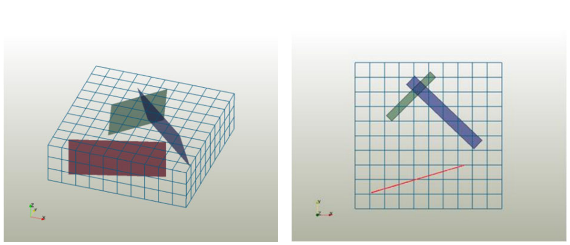
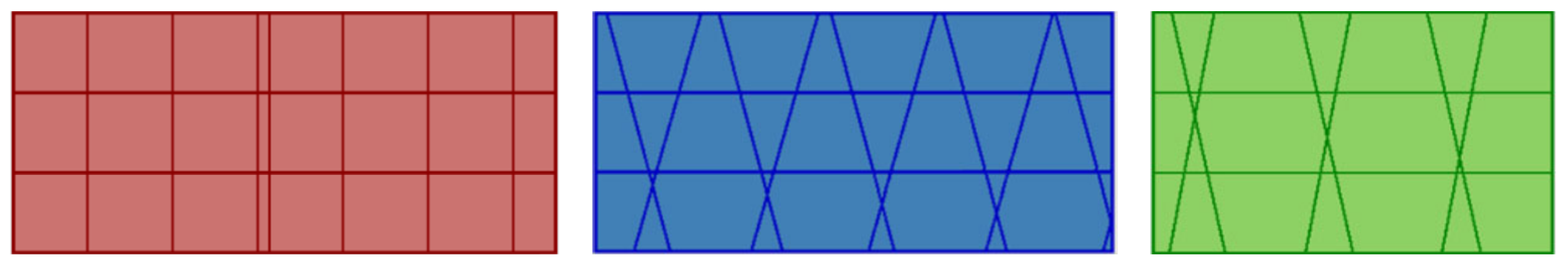
2.1. Embedded Discrete Fracture Model (EDFM)

The commonly used methods to simulate fluid flow in reservoirs include the double-medium model [44,45], discrete fracture model [46,47], and embedded discrete fracture model [48]. In the double-medium model, the ideal state is suitable only for reservoirs that have great connectivity between fractures. In the discrete fracture model, the reservoir is divided by an unstructured grid. When simulating the flow of some complex fracture models, the closer to the fracture and the larger the model calculation, the less sufficient the convergence becomes.
The embedded discrete fracture model overcomes the shortcomings of the double-medium model and discrete fracture model. It not only highlights the flow characteristics of a single fracture but also greatly reduces the amount of calculation. Therefore, this paper selected the embedded discrete fracture module (HFM) in MRST (MATLAB Reservoir Simulation Toolbox) to simulate the production of fractured reservoirs [49,50].
EDFM has two main characteristics; one is the method of meshing, and the other is the method of coupling the fracture to the matrix [51,52,53,54]. The embedded discrete fracture model uses a structured grid to divide the reservoir matrix, while for complex fractures, it uses an unstructured grid. Figure 1 illustrates fractures using EDFM, and Figure 2 illustrates the results of the fracture in the above model.

2.2. Hydraulic Fracture Network Geometry Model Design

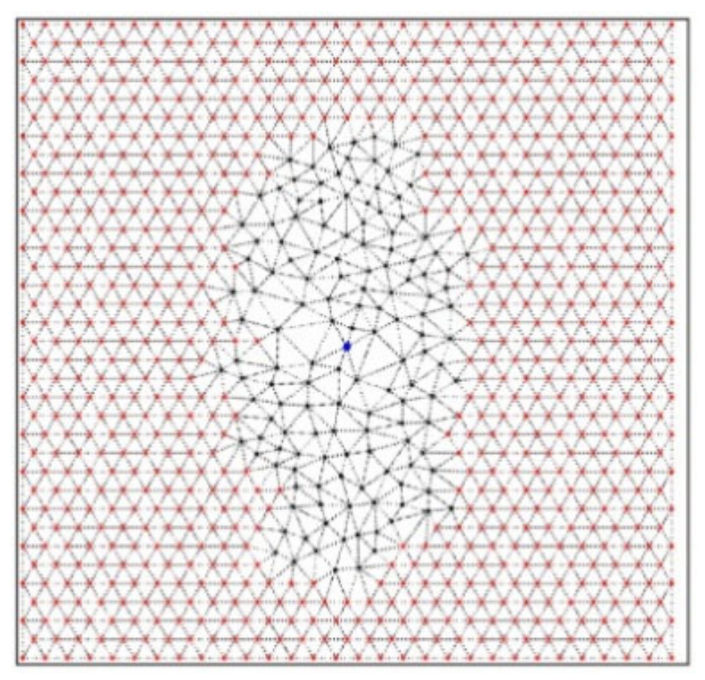
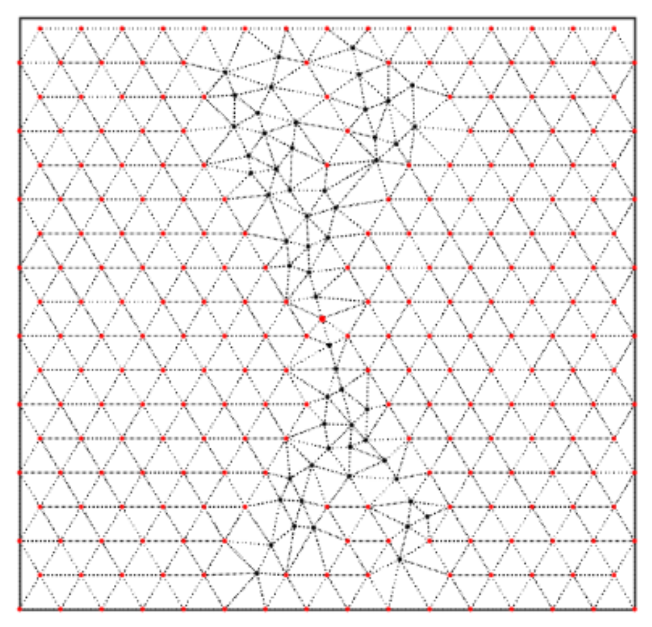
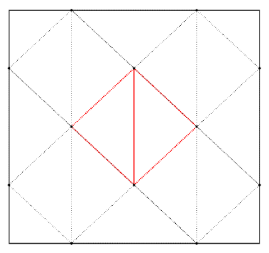
2.2.1. The Delaunay Triangulation Method

The microseismic technique is the most commonly used monitoring method for fractured reservoirs. In this section, the microseismic point set obtained from the monitoring was taken as the constraint of the fracture network. The Delaunay triangulation method [55] was used to divide the microseismic points into possible fracture network structures.
The microseismic points were the set of subdivision points in the monitoring area. For reservoir areas not detected by microseismic monitoring, some regular point sets were defined, which are shown as the red points in Figure 3. The regular points and microseismic points outside the monitoring area constituted a set of points to be subdivided as a constraint of the fracture network inversion.
Figure 3 is a schematic diagram of a 600 m × 600 m reservoir after subdivision. The irregularly distributed points in the middle are the microseismic points detected, and the microseismic areas are the areas where fractures were observed. The area of the peripheral regular point is the area where the fractures may not be detected by microseismic monitoring. The network structure after subdivision was regarded as a possible form of the fracture network, based on which a complex fracture network generation method was constructed in this paper.

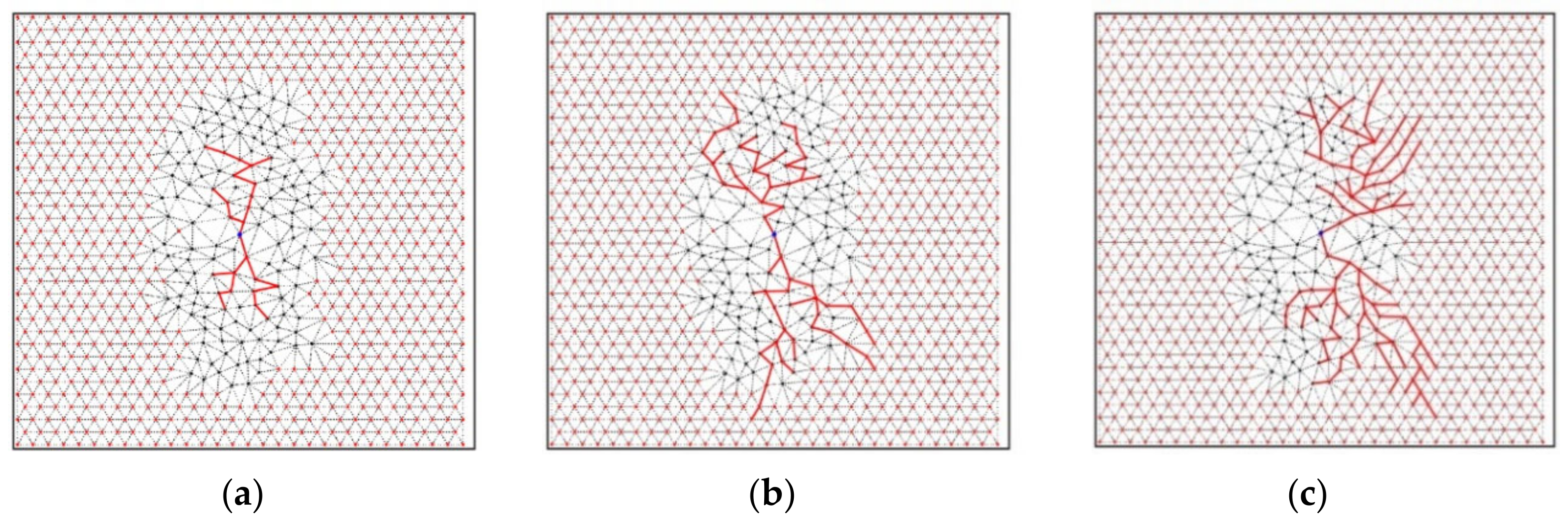
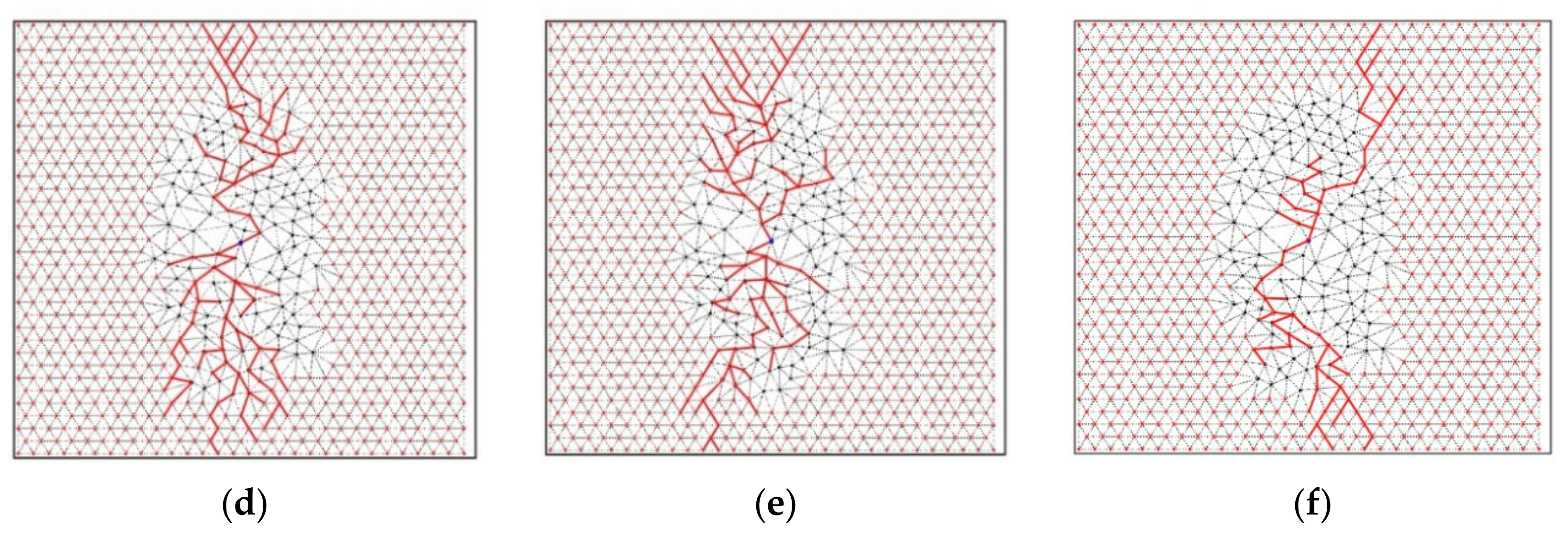
2.2.2. Complex Hydraulic Fracture Network Generation Method Based on the L-System

Current studies have shown that fractures have the characteristics of tree-like fractals, and the L-system [56] is often used to simulate the shape of fractal trees. Therefore, a fracture network generation rule based on L-system was established.
To increase the complexity of the fracture network, we established a random mechanism of L-system character substitution in which a random number c was defined. Different character replacement rules were defined within the range of different random numbers. In each iteration, the random numbers were generated again. The character replacement rules were as follows:
  • If c > 0.75, F → F[+F][−F]F;
  • If 0.75 > c > 0.50, F → F;
  • If 0.50 > c > 0.25, F → F − F;
  • If 0.25 > c, F → F + F.
Figure 4 shows the fracture network morphology obtained through different iterations based on the previously established subdivided reservoir structure. It can be seen from the figure that the range and complexity of the fracture network increased with the increase of the number of iterations. It should be noted here that the fracture network generated by a high number of iterations is not necessarily larger than that generated by a low number of iterations, because repeated fracture segments appear in the final result generated by the fracture network. Therefore, repeated fracture segments in the fracture network were removed in the processing of the final fracture network generated, as shown in Figure 4f. However, a high number of iterations had a higher probability of generating a fracture network with a higher degree of complexity, and such results were easier to extend beyond the microseismic monitoring results in the reservoir.
In choosing the next point in the process of seismicity, we considered the same fracture produced by the microseismic point on most of the relatively close, and we considered that microseismic points generated by different fracture segments may be far. We therefore established our model based on the choice of the distance criterion; i.e., points close to the current candidate microseismic point were selected during generation as being at greater risk of being fracture points; meanwhile, faraway points were less likely to be fracture points based on the candidate microseismic point. In the actual operation, the Euclidean distance between each candidate point and the current microseismic point was calculated, the reciprocal was taken, and this reciprocal of the distance was normalized into the probability for the selected candidate point.

3. Multiobjective Fracture Network Inversion Algorithm Based on Decomposition (MOFNIAD)

3.1. The Bayesian Objective Function

Bayesian theory is a statistical prediction method that introduces the prior information of the problem into the method [57]. In the petroleum field, it is often used to construct the objective function in the historical fitting method. In the history-matching method, the sedimentary facies of the reservoir are used as the prior information of reservoir geology inversion [58]. Bayesian theory can be summarized as follows:
p B | A = p A | B * p B
Assuming that the problem is subject to a Gaussian distribution with a priori information as the mean value, then the probability p(m) of the problem is:
p m = 1 2 π C m e m m p r 2 2 C m exp 1 2 m m p r T C m 1 m m p r
When the parameter m is given, the probability distribution function of the observed data is the probability distribution function of the observation error:
p d o b s | m = 1 2 π C D e d o b s g ( m ) 2 2 C D exp 1 2 d o b s g ( m ) T C D 1 d o b s g ( m )
where m represents the desired parameter, which in this paper was the candidate option of subspace, namely the microseismic monitoring results and the production data; mpr represents prior information; Cm represents the covariance matrix of prior information, and its diagonal is the variance of the desired parameter; CD represents the error of observed data; dobs represents real observation data; g(m) represents the forward modeling results corresponding to different parameters, which in this paper were the seismic data of the reservoir under the production of different fracture networks detected by microseismic monitoring.
According to Bayesian theory, under the premise that the true model is that which actually occurred, the probability distribution function p(m|dobs) of the request parameter was as follows:
p m | d o b s p d o b s | m * p m exp 1 2 d o b s g ( m ) T C D 1 d o b s g ( m ) 1 2 m m p r T C m 1 m m p r
Networks of greater probability demand more closely to the true model parameters. Therefore, the inversion of the target maximizes the probability p(m|dobs), so the objective function was simplified as:
f m = 1 2 d o b s g ( m ) T C D 1 d o b s g ( m ) + 1 2 m m p r T C m 1 m m p r
In the optimization process, the parameter that minimizes the objective function f(m) should be obtained. When the objective function reaches the minimum, it can not only make the observation data fit best, but also conform to the prior model.

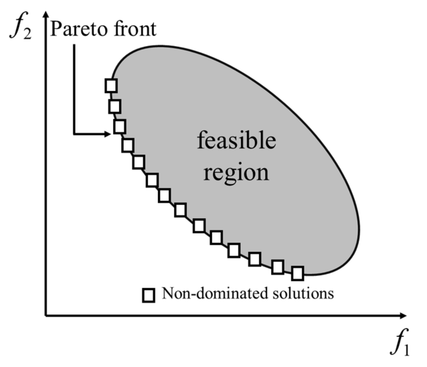
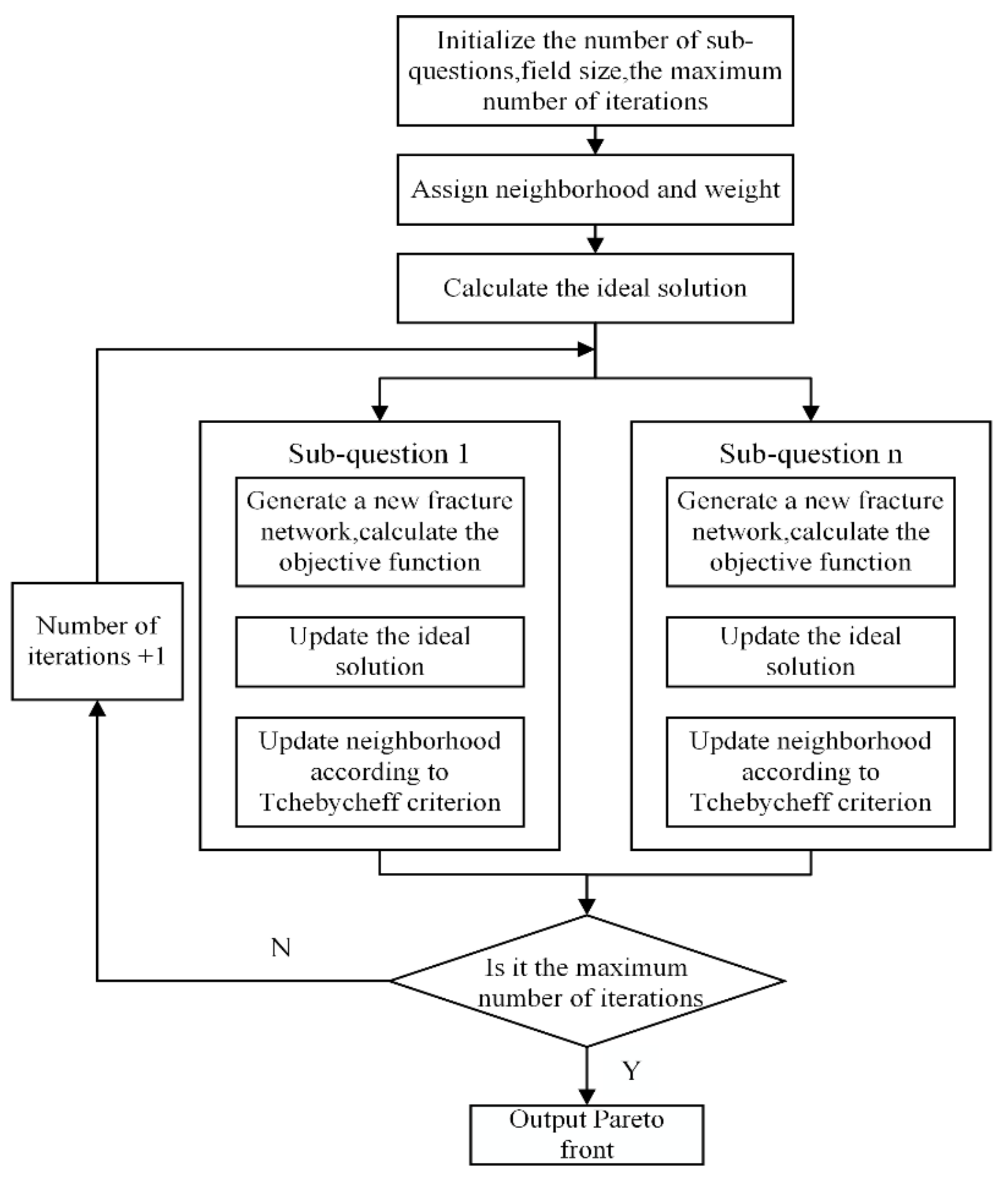
3.2. Multiobjective Fracture Network Inversion Algorithm Based on Decomposition

A general multiobjective minimization problem that aims to simultaneously optimize more than one conflicting objective can be formulated as
min F ( x ) = [ f 1 ( x ) , f 2 ( x ) , , f m ( x ) ] T s . t . x X
where x = (x1, x2, …, xd)T is the optimization vector, X is the feasible region in d-dimensional decision space, m is the number of objective functions, and F: RdRm is an objective vector.
Multiobjective algorithms are mainly used to solve optimization problems with more than one objective function, where objective functions are conflicting objectives [59,60,61,62]. Using a multiobjective optimization algorithm, solutions with different target ratios can be optimized. For a multiobjective problem with two objective functions, the feasible solution that satisfies the multiobjective problem constitutes the feasible region of the multiobjective problem. The feasible region is usually an irregular closed plane, and the boundary curve inside the feasible region near the ideal side of the multiobjective problem is called the Pareto front. The solutions on this front are optimal and nondominated. The dominance relationship is defined as
x 1 x 2     if   and   only   if i { 1 , 2 , , m } , f i ( x 1 ) f i ( x 2 ) i { 1 , 2 , , m } , f i ( x 1 ) < f i ( x 2 )
where refers to the dominance relationship and x1 is said to dominate x2. The optimization objective of the multiobjective algorithm is to find the Pareto front in the feasible region, and then select the required solution from the Pareto front according to different needs. Figure 5 illustrates the Pareto front for a biobjective problem.
The two objectives used in this paper were the degree of fit between the fracture network and the microseismic detection results and the degree of fit between the fracture network and the real fracture production data during the production process. Because of the error of microseismic monitoring, the change of reservoir pressure during the production process, the ambiguity of fracture inversion, and other factors, the two objective functions were directly proportional in a nonstrict sense. The multiobjective optimization algorithm is roughly divided into two parts, one to maintain the diversity of the multiobjective problem solution and the other to maintain the uniformity of the Pareto front. In this paper, the L-system-based fracture network production method was used to maintain the diversity of solutions, and the decomposition method was used to maintain the uniformity of Pareto front solutions.
The decomposition method transforms the multiobjective problem into multiple scalarization optimization problems according to different objective weights so that the multiobjective algorithm can solve a finite number of solutions on the Pareto front using the decomposition method. The Chebyshev method was used as the decomposition method:
min   g   =   max 1 i m λ i | f i ( x )     z i * |
where zi* represents the optimal objective function value of the objective i in all solutions and z* is a collection of the optimal values of each objective function.
The principle of the Chebyshev method is to minimize the maximum value of each target and optimal value under different weights. In the optimization process, the optimized solution continuously approaches the Pareto front around the weight vector. The Pareto front solution obtained by this method depends on the choice of weights.
The multiobjective fracture network inversion algorithm established in this section combines the fracture network generation method with the Chebyshev decomposition method. The algorithm allocates the number of subproblems and evenly distributes the weight of different objectives in each subproblem, sets the number of neighborhoods for each subproblem, and assigns neighborhoods according to the Euclidean distance of each subproblem. The neighborhood is set to reduce the amount of calculation for updating the subproblem in each iteration. The optimal solution in each subproblem is updated based on the information in the neighborhood, and each subproblem continuously approaches the optimal solution on the Pareto front through the Chebyshev method. For the calculation of the objective function, this paper took the degree of fit of the microseismic monitoring results and the degree of fit of the production data as its two objective functions. The number of microseismic sources covered by different fracture networks was used to indicate the degree of fit of the microseismic monitoring results. The embedded discrete fracture model was used to simulate the flow and production results of different fracture networks, and the absolute value of the difference between the production data of the calculated fracture networks and the real production data was calculated to indicate the degree of fit of the production data. The maximum number of iterations was used as the condition for the algorithm to stop. Figure 6 illustrates the algorithm flowchart.

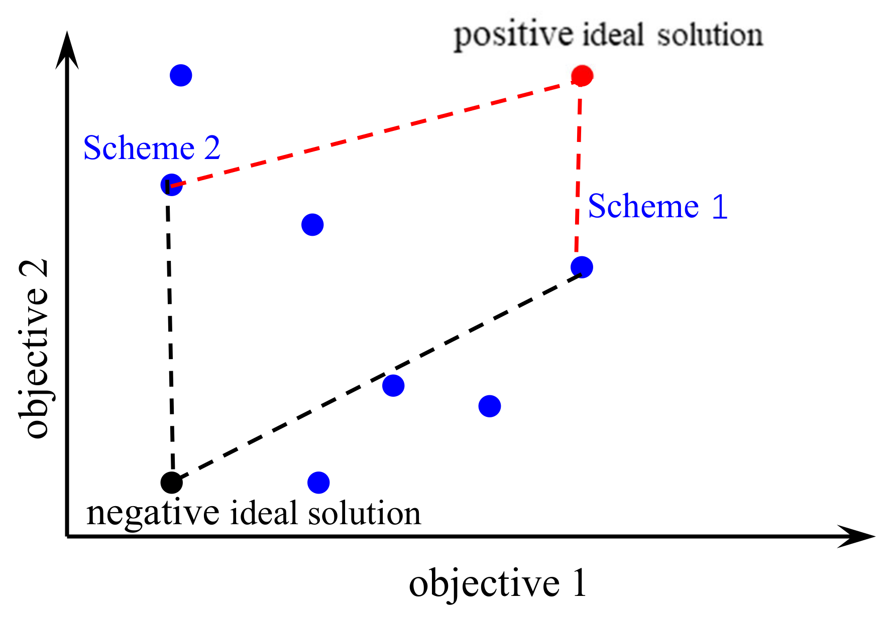
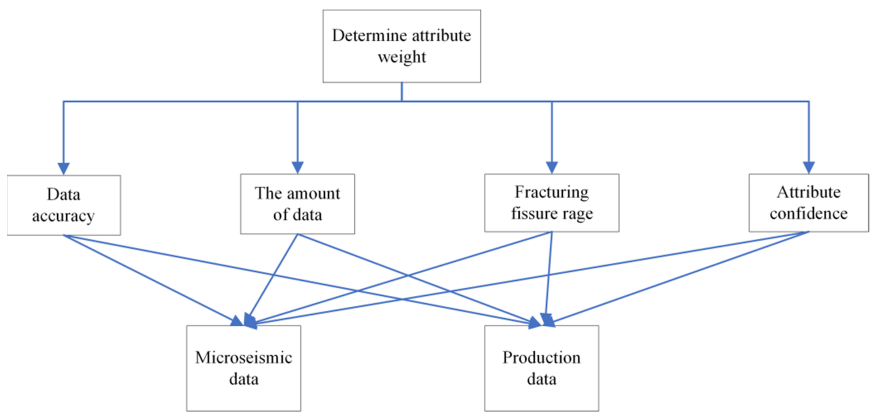
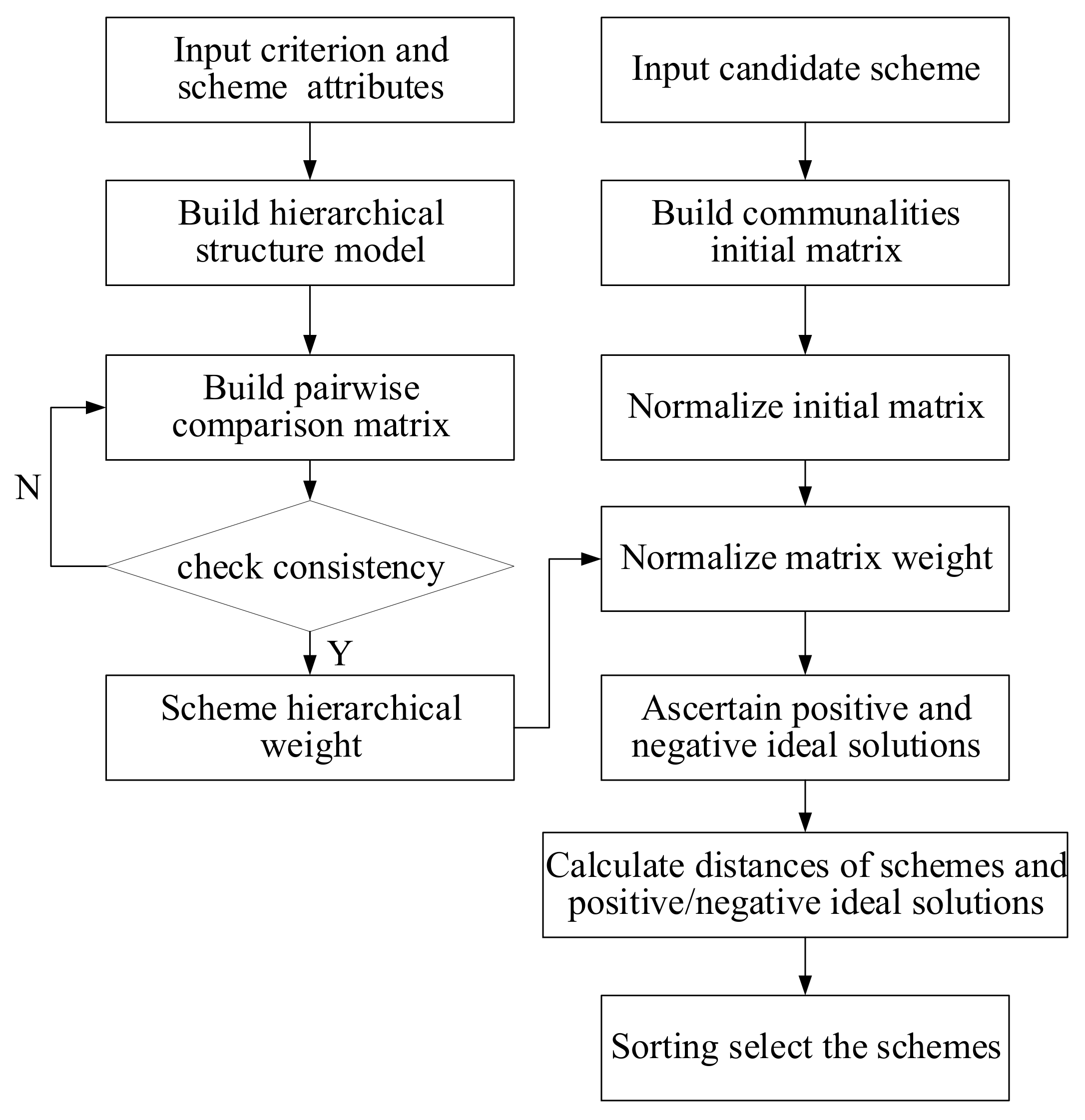
3.3. Multiple Criteria Decision Making

Through the established algorithm, we could optimize to obtain a variety of solutions that met the proportions of different attributes. The multiattribute decision-making method was needed for the decision making of these schemes in different situations.
The TOPSIS (technique for order preference by similarity to an ideal solution) helps decision makers to choose the best solution in different situations by comparing the gap between different schemes and the most ideal scheme and the worst scheme. This method makes full use of the information of different attributes to help decision makers quickly find the best solution, and there are fewer restrictions on attributes.
Figure 7 illustrates the principle of this method. The maximization of the properties of the problem is in the ideal state. Compared with scheme 2, scheme 1 is closer to the positive ideal solution, so scheme 1 is more applicable than scheme 2.
The analytic hierarchy process (AHP) is a multiple-criteria decision-making process that is used to set priorities among different attributes. The AHP has been widely used to reflect the importance, or relative weight, of the factors associated with priorities. The AHP method consists of three basic steps: first, the problem is broken down and structured into a hierarchy of subproblems; second, the data are collected and measured through pairwise comparisons of the attributes; and finally, the priority weights of factors or items in each level are calculated. A judgment or comparison consists of a numerical representation of a relationship between two elements that share a common parent. The set of all relative comparisons is then reported in a square matrix in which the elements are compared with each other. Figure 8 illustrates a schematic diagram of the hierarchy structure in AHP.
In this paper, considering the advantages and disadvantages of the ranking method that approaches the ideal solution, a multiattribute decision-making method that combined the TOPSIS and AHP was established [63].
To reduce the judgment error of the TOPSIS, AHP analysis was used for the sorting method of approximation to the ideal solution scheme. The weights of attributes in the AHP were used to construct the hierarchical structure of the model and to set the target for calculating the weights of every scheme as close as possible to the ideal solution layer in the sorting method solution properties. In this paper, the objective function was used in the multiobjective fracture inversion algorithm, and the criterion layer was defined as the index. The latter was selected to make it easy to judge the weight of the scheme layer, so that the decision maker can more accurately select a scheme without rich experience and with minimal use of subjective judgment. Figure 9 illustrates the flowchart of the established decision-making method. Multiple fracture network schemes optimized by the multiobjective fracture network inversion algorithm were taken as the input of candidate schemes. The judgment criteria and the objective function used in the multiobjective fracture network inversion algorithm were defined as the inputs of criteria and scheme attributes.

4. Results and Discussion

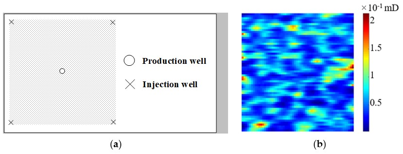
4.1. Reservoir Model

A 600 × 600 m low-permeability, heterogeneous oil reservoir model was established. This oil reservoir model was developed by using the five-point method. Four injection wells are located in the four corners of the reservoir, and one fractured production well is located in the center of the reservoir. Figure 10 shows the well locations in the reservoir and the permeability of the reservoir.
The modeled reservoir has adopted fracturing and stimulation measures. The simulated reservoir has been produced for 5 years after fracturing. The embedded discrete fracture model was divided into 68-step simulations. The reservoir simulation was carried out with constant production bottom flow pressure. It was assumed that the formation contained only oil and water two phases. The specific reservoir parameters are shown in Table 1. The difference between case 1 and case 2 lay in the injection rate of the injection well. The EDFM was used to simulate the production of the fractured reservoir.

4.2. Case 1

For the shape of the real fracture, the method of using the L-system to characterize fracture morphology in the references was used to randomly generate a real fracture. Microseismic points with smaller errors reflected the approximate distribution of fracture. Smaller interference was added that conformed to the normal distribution, and regular point division as added.
Applying the above generation method to independently generate fracture networks of different shapes on both sides with the production well in the center, the actual fracture, shown in Figure 11, was generated. A point was randomly generated in the generated real fracture segment to indicate the location of the microseismic point, while the midpoint of each fracture segment represented the distribution of the microseismic points generated by the simulation. To consider the errors in the microseismic monitoring process, disturbances that conformed to the normal distribution were added to the generated microseismic point distribution to simulate the set of microseismic points in the fracturing area. The distribution of simulated microseismic point sets and the distribution of microseismic point sets after adding errors are shown in Figure 12. The cross marks represent the initial generated microseismic point sets, and the dots represent the distribution of microseismic point sets after adding random interference. Based on the generated microseismic points, regular points were added to the external area, and the points existing in the reservoir were Delaunay triangulated. The interval of adding regular points was 40 m. The shape after division was as shown. The red dots indicate the added regular points, and the black dots indicate the distribution of the set of microseismic points after adding the error.
After dividing the microseismic points and the added regular points in the reservoir, using the coverage of the microseismic monitoring results and the fitting degree of the production data as the objective function, the MOFNIAD method proposed in this paper was used to invert the fracture morphology. The coverage of the microseismic monitoring results was expressed by the number of microseismic points covered by the generated fracture network, and the fitting degree of the production data used the absolute value of the difference between the production data of the simulated and real fracture networks. For the production data of the real fracture model, the embedded discrete fracture model introduced previously was used to simulate the production of the real fracture network. The saturation field and production data of the reservoir at a certain time after fracturing are shown in Figure 13.
The number of multiobjective subproblems was 50, and the maximum iteration number of the multiobjective inversion algorithm was 100. The Pareto front obtained by the final multiobjective inversion is shown in Figure 14. In this example, due to the small error of microseismic monitoring results, the number of microseismic points covered by the actual fracture morphology was highest, and the fitting degree of the microseismic monitoring results was basically proportional to the fitting degree of the production data. Therefore, the Pareto front was narrow, and only three schemes that were similar to the real fracture were optimized. Figure 15, Figure 16 and Figure 17 show comparisons of the fracture morphology and production data of these three schemes.
To further evaluate the similarity between the fracture network and the real model in the optimization scheme theoretically, this paper defined the allowable error range. The fracture inversion method is a fracture network constructed on the basis of the Delaunay triangle. If the fracture segment obtained by the inversion belonged to the triangle where the real fracture segment was located, the fracture segment of the inversion was considered as within the acceptable error range. Figure 18, in which the solid line is the real fracture segment and the dotted line is the fracture segment within the acceptable error range, shows the acceptable error range. Figure 19 shows the distribution range of fracture segments within the allowable error of the theoretical optimal model fracture network.
Figure 20 shows the error area evaluation results based on the fracture networks of schemes 1, 2, and 3, respectively. The red line represents the coincident fracture segment with the theoretical optimal fracture network, the orange line represents the allowable error, and the green line represents that the error was larger than allowed.
The error evaluation results of the three schemes based on the theoretical optimal fracture network are shown in Figure 21, where the red and orange lines’ meanings are the same as those in Figure 20. The blue line represents the fracture segments in the theoretically optimal fracture network that were not obtained by inversion.
The fracture network in scheme 1 was basically within the allowable error range. However, judging from the evaluation results based on the theoretical optimal fracture network, many fracture segments were not within the allowable error range. In scheme 3, the fracture network had more fracture segments within the allowable error range of the theoretical optimal fracture network, but the number of redundant fracture segments was also large. The fracture network in scheme 2 is between scheme 1 and scheme 3. Most of the three optimized fracture networks were within the allowable error range and were basically close to the theoretical optimal fracture network form.

4.3. Case 2

Research has shown that in the technology of microseismic monitoring, the process of picking up microseismic signals, obtaining velocity models, constructing forward models, constructing objective functions, and selecting optimization algorithms brings errors to the source location; these errors can be as much as 100 m. For this reason, it is necessary to consider the large error of microseismic monitoring results. Case 1 used microseismic monitoring results with a small error to verify the fracture network inversion method proposed in this paper. Case 2 considered another case where the error between microseismic monitoring results and real fracture morphology is large. The feasibility of applying MOFNIAD was considered. In Case 2, the morphology of the actual fracture was basically the same as that in Case 1, but the strike of the fracture was adjusted. Meanwhile, the microseismic points close to the fractured well were added with less interference, while the microseismic points set far away from the fractured well were added with more interference.
Figure 22a shows the real fracture network. Figure 22b shows the comparison of the distribution of microseismic points without interference and after interference. The blue dots represent points without interference, and the black dots represent points after interference.
Figure 23 shows the obtained Pareto front. In this case, the microseismic monitoring results have a large error, so the coverage degree of the microseismic monitoring results and the fit degree of the production data are two conflicting objectives. The greater the coverage of microseismic results, the greater the gap between the fracture network and the real fracture network, and the more obvious the difference in the degree of fitting of production data. When the microseismic monitoring results have a poor fit, the production data may fit better with the actual production data. The Pareto front obtained in this case was wider than that in the previous section, and the optimal solution had a larger range and more numbers on the two optimization objectives.
The schemes were named in the order of the abscissa on the Pareto frontier. The model with the best production data fit was the first scheme, and the tenth scheme had the best coverage of the microseismic monitoring results. In this case, there was no theoretical optimal model that dominated all solutions. When the inversion fracture is very close to the real fracture, the obtained production data has little difference from the real production data. In other words, the objective function of production data fit is smaller. This scheme has a dominant relationship with the solution within a small range of production data. Therefore, when the number of iterations is large enough, the scheme that is theoretically closest to the real fracture shape is the scheme with the smallest abscissa on the Pareto front (the first scheme). The higher the degree of microseismic coverage, the greater the possibility of deviation from the true fracture shape.
Figure 24 shows the fracture morphology in the first and second schemes. In schemes 1 and 2, due to the better fit of the microseismic monitoring results, the fracture network shape extended to the microseismic monitoring area, slightly deviating from the real fracture shape. Figure 25 shows the fracture shapes in schemes 3 and 10. The fracture network form in scheme 10 deviates significantly from the real fracture network form.
From the comparison between the production data in Figure 26 and Figure 27, since the area covered by the fracture in scheme 10 was larger, the simulated oil production was higher than the real production data.
Thus, it can be seen that the scheme theoretically closest to the real fracture network was scheme 1; it fits the production best. The allowable error range defined in the previous case was applied to evaluate the similarity between fracture morphology and the real fracture network in scheme 1. It can be seen from Figure 28 and Figure 29 that most of the fracture segments of the fracture network in scheme 1 were within the allowable error range.
The optimization results of this case had a scheme that was far from the real model, such as scheme 10 with a larger coverage of microseismic results. Therefore, a multischeme decision-making method was used to choose a better scheme.
When the two objectives of optimization are proportional and the number of algorithm iterations is large enough, the optimized Pareto frontier is narrow and there are fewer solutions. If the two objectives are conflicting, as in this case, when the number of iterations of the algorithm is sufficient, the optimized Pareto front range is wider and there are more solutions. The following figure shows a comparison of the Pareto front (triangular mark) obtained from the case of microseismic monitoring with small errors and the Pareto front (dots) from the case of microseismic monitoring with large errors discussed in this section. Therefore, according to the multischeme decision-making method established in this article, one can first judge the weighting tendency of the optimization objective based on the optimized Pareto front. If the Pareto front range is wide, the relationship of the optimized targets is obviously in conflict. When using the analytic hierarchy process to determine the target weight, the accuracy or attribute confidence should be more inclined to the production data. In practice, the error in the production data monitoring results is small.
The above section shows a case of a multischeme decision-making method. It inclined toward production data in terms of accuracy and attribute confidence. The weights of the fitting degree of production data and the degree of microseismic coverage calculated by the AHP method were (0.78, 0.22), respectively. The best solution presented was scheme 1.

5. Conclusions

This paper proposes a new fracture network inversion method by using a decomposition-based multiobjective fracture network inversion algorithm. According to the error conditions of microseismic monitoring results, two different test cases were established. The MOFNIAD was used in these cases and obtained similar schemes to the real fracture network shape. If there were many optimization result schemes, the method was inclined to produce data using multiple decision methods. The results of the cases verified the characteristics and inversion effects of the fracture inversion method proposed in this paper.

Author Contributions

Conceptualization, L.Z., L.X., and K.Z.; data curation, L.X. and C.C.; formal analysis, L.Z. and C.C.; funding acquisition, L.Z. and K.Z.; methodology, L.Z. and K.Z.; project administration, L.Z. and K.Z.; software, L.X.; supervision, L.Z. and K.Z.; validation, L.Z. and C.C.; writing—original draft, L.X.; writing—review and editing, J.Q., J.S., X.Z. and Q.D. All authors have read and agreed to the published version of the manuscript.

Funding

This research was funded by the National Natural Science Foundation of China under Grants 51722406, 61573018, 51874335, and 52074340; the Natural Science Foundation of Shan Dong Province under Grants JQ201808, ZR2015EL014, and ZR2019MEE101; the National Science and Technology Major Project of China under Grant 2016ZX05025001-006; and the Fundamental Research Funds for the Central Universities under Grant 18CX02097A.

Institutional Review Board Statement

Not applicable.

Informed Consent Statement

Not applicable.

Data Availability Statement

Data is contained within the article.

Conflicts of Interest

The authors declare no conflict of interest.

References

  1. Zhang, K.; Zhao, X.; Zhang, L.; Zhang, H.; Wang, H.; Chen, G.; Zhao, M.; Jiang, Y.; Yao, J. Current status and prospect for the research and application of big data and intelligent optimization methods in oilfield development. Zhongguo Shiyou Daxue Xuebao (Ziran Kexue Ban)/J. China Univ. Pet. (Ed. Nat. Sci.) 2020, 44, 28–38. [Google Scholar]
  2. Xu, X.; Wei, Z.; Ji, Q.; Wang, C.; Gao, G. Global renewable energy development: Influencing factors, trend predictions and countermeasures. Resour. Policy 2019, 63, 101470. [Google Scholar] [CrossRef]
  3. Krohn, C.E. Fractal measurements of sandstones, shales, and carbonates. J. Geophys. Res. Solid Earth 1988, 93, 3297–3305. [Google Scholar] [CrossRef]
  4. Ho, W. Integrated analytic hierarchy process and its applications—A literature review. Eur. J. Oper. Res. 2008, 186, 211–228. [Google Scholar] [CrossRef]
  5. Hwang, C.L.; Yoon, K. Multiple Attribute Decision Making Methods and Applications A State-of-the-Art Survey; Springer: Berlin/Heidelberg, Germany, 1981; Volume 186. [Google Scholar]
  6. Meyer, B.R.; Bazan, L.W. A Discrete Fracture Network Model for Hydraulically Induced Fractures—Theory, Parametric and Case Studies. In Proceedings of the SPE Hydraulic Fracturing Technology Conference, The Woodlands, TX, USA, 24–26 January 2011. [Google Scholar]
  7. Maxwell, S.C.; Urbancic, T.I.; Steinsberger, N.; Zinno, R. Microseismic Imaging of Hydraulic Fracture Complexity in the Barnett Shale. In Proceedings of the SPE Annual Technical Conference and Exhibition, San Antonio, TX, USA, 29 September–2 October 2002. [Google Scholar]
  8. Miettinen, K. Nonlinear Multiobjective Optimization; Springer: Boston, MA, USA, 1998. [Google Scholar]
  9. Dahi Taleghani, A. Analysis of hydraulic fracture propagation in fractured reservoirs: An improved model for the interaction between induced and natural fractures. Ph.D. Thesis, The University of Texas, Austin, TX, USA, May 2009. [Google Scholar]
  10. Sasaki, S. Characteristics of microseismic events induced during hydraulic fracturing experiments at the Hijiori hot dry rock geothermal energy site, Yamagata, Japan. Tectonophysics 1998, 289, 171–188. [Google Scholar] [CrossRef]
  11. Hainey, B.W.; Keck, R.G.; Smith, M.B.; Lynch, K.W.; Barth, J.W. On-site Fracturing Disposal of Oilfield-Waste Solids in Wilmington Field, California. SPE Prod. Facil. 1999, 14, 83–87. [Google Scholar] [CrossRef]
  12. Raaen, A.M.; Skomedal, E.; Kjørholt, H.; Markestad, P.; Økland, D. Stress determination from hydraulic fracturing tests: The system stiffness approach. Int. J. Rock Mech. Min. Sci. 2001, 38, 529–541. [Google Scholar] [CrossRef]
  13. Murdoch, L.C.; Slack, W.W. Forms of Hydraulic Fractures in Shallow Fine-Grained Formations. J. Geotech. Geoenvironmental Eng. 2002, 128, 479–487. [Google Scholar] [CrossRef]
  14. Olson, D.L. Comparison of weights in TOPSIS models. Math. Comput. Model. 2004, 40, 721–727. [Google Scholar] [CrossRef]
  15. Nordgren, R.P. Propagation of a Vertical Hydraulic Fracture. Soc. Pet. Eng. J. 1972, 12, 306–314. [Google Scholar] [CrossRef]
  16. Olson, J.E. Multi-fracture propagation modeling: Applications to hydraulic fracturing in shales and tight gas sands. In Proceedings of the 42nd U.S. Rock Mechanics Symposium (USRMS), San Francisco, CA, USA, 29 June–2 July 2008. [Google Scholar]
  17. Perkins, T.K.; Kern, L.R. Widths of Hydraulic Fractures. J. Pet. Technol. 1961, 13, 937–949. [Google Scholar] [CrossRef]
  18. Barree, R.D.; Fisher, M.K.; Woodroof, R.A. A Practical Guide to Hydraulic Fracture Diagnostic Technologies. Proceedings of th SPE Annual Technical Conference and Exhibitioen, San Antonio, TX, USA, 29 September–2 October 2002. [Google Scholar]
  19. Cipolla, C.L.; Wright, C.A. State-of-the-Art in Hydraulic Fracture Diagnostics. In Proceedings of the SPE Asia Pacific Oil and Gas Conference and Exhibition, Brisbane, Australia, 16–18 October 2000. [Google Scholar]
  20. Germanovich, L.N.; Astakhov, D.K.; Mayerhofer, M.J.; Shlyapobersky, J.; Ring, L.M. Hydraulic fracture with multiple segments I. Observations and model formulation. Int. J. Rock Mech. Min. Sci. 1997, 34, 97.e1–97.e19. [Google Scholar] [CrossRef]
  21. Develi, K.; Babadagli, T. Quantification of Natural Fracture Surfaces Using Fractal Geometry. Math. Geol. 1998, 30, 971–998. [Google Scholar] [CrossRef]
  22. Geertsma, J.; De Klerk, F. A Rapid Method of Predicting Width and Extent of Hydraulically Induced Fractures. J. Pet. Technol. 1969, 21, 1571–1581. [Google Scholar] [CrossRef]
  23. Ren, L.; Zhao, J.; Hu, Y. Hydraulic fracture extending into network in shale: Reviewing influence factors and their mechanism. Sci. World J. 2014, 2014, 847107. [Google Scholar] [CrossRef] [PubMed]
  24. Xue, Z.; Yang, L.; Cui, L. Roundup of Fracture Detection Techniques During Hydraulic Fracturing Operation at Home & Abroad. Low Permeability Oil Gas Fields 2010, 3, 90–95. [Google Scholar]
  25. Liu, Z.; Sa, L.; Wu, F.; Dong, S.; Li, Y. Microseismic monitor technology status for unconventional resource E&P and its future development in CNPC. Shiyou Diqiu Wuli Kantan/Oil Geophys. Prospect. 2013, 48, 843–853. [Google Scholar]
  26. Chen, Y.; Hong, L.; Yalin, L.; Furong, W.; Guangming, H.; Chunhua, C. The precision analysis of the microseismic location. Prog. Geophys. 2013, 28, 800–807. [Google Scholar]
  27. Wright, C.A.; Weijers, L.; Davis, E.J.; Mayerhofer, M. Understanding Hydraulic Fracture Growth: Tricky but Not Hopeless. In Proceedings of the SPE Annual Technical Conference and Exhibition, Houston, TX, USA, 3–6 October 1999. [Google Scholar]
  28. Shewchuk, J.R. Delaunay refinement algorithms for triangular mesh generation. Comput. Geom. 2002, 22, 21–74. [Google Scholar] [CrossRef] [Green Version]
  29. Vaidya, O.S.; Kumar, S. Analytic hierarchy process: An overview of applications. Eur. J. Oper. Res. 2006, 169, 1–29. [Google Scholar] [CrossRef]
  30. Weng, X.; Kresse, O.; Cohen, C.; Wu, R.; Gu, H. Modeling of Hydraulic Fracture Network Propagation in a Naturally Fractured Formation. In Proceedings of the SPE Hydraulic Fracturing Technology Conference, The Woodlands, TX, USA, 24–26 January 2011. [Google Scholar]
  31. Wendong, W. Fractal-based Multi-stage Hydraulically Fracture Network Characterization and Flow Modeling. Ph.D. Thesis, China University of Petroleum (East China), Dongying, China, December 2015. [Google Scholar]
  32. Chaoyang, H.; Chi, A.; Fengjiao, W. Distribution simulation of branched hydraulic fracture based on fractal theory. Pet. Geol. Recovery Effic. 2016, 23, 122–126. [Google Scholar]
  33. Zhang, Q.; Li, H. MOEA/D: A Multiobjective Evolutionary Algorithm Based on Decomposition. IEEE Trans. Evol. Comput. 2007, 11, 712–731. [Google Scholar] [CrossRef]
  34. Xu, W.; Thiercelin, M.; Ganguly, U.; Weng, X.; Gu, H.; Onda, H.; Sun, J.; Le Calvez, J. Wiremesh: A Novel Shale Fracturing Simulator. In Proceedings of the International Oil and Gas Conference and Exhibition in China, Beijing, China, 8–10 June 2010. [Google Scholar]
  35. Yang, F.; Ning, Z.; Liu, H. Fractal characteristics of shales from a shale gas reservoir in the Sichuan Basin, China. Fuel 2014, 115, 378–384. [Google Scholar] [CrossRef]
  36. Zhang, D.; Yang, T. Environmental impacts of hydraulic fracturing in shale gas development in the United States. Pet. Explor. Dev. 2015, 42, 876–883. [Google Scholar] [CrossRef]
  37. Yushi, Z.; Shicheng, Z.; Tong, Z.; Xiang, Z.; Tiankui, G. Experimental Investigation into Hydraulic Fracture Network Propagation in Gas Shales Using CT Scanning Technology. Rock Mech. Rock Eng. 2016, 49, 33–45. [Google Scholar] [CrossRef]
  38. Zhou, Z.; Su, Y.; Wang, W.; Yan, Y. Application of the fractal geometry theory on fracture network simulation. J. Pet. Explor. Prod. Technol. 2017, 7, 487–496. [Google Scholar] [CrossRef] [Green Version]
  39. Zhang, K.; Zhang, J.; Ma, X.; Yao, C.; Zhang, L.; Yang, Y.; Wang, J.; Yao, J.; Zhao, H. History Matching of Naturally Fractured Reservoirs Using a Deep Sparse Autoencoder. SPE J. 2021, 26, 1700–1721. [Google Scholar] [CrossRef]
  40. Xue, X.; Zhang, K.; Tan, K.C.; Feng, L.; Wang, J.; Chen, G.; Zhao, X.; Zhang, L.; Yao, J. Affine Transformation-Enhanced Multifactorial Optimization for Heterogeneous Problems. IEEE Trans. Cybern. 2020, 1–15, in press. [Google Scholar] [CrossRef] [PubMed]
  41. Ma, X.; Zhang, K.; Zhang, L.; Yao, C.; Yao, J.; Wang, H.; Jian, W.; Yan, Y. Data-Driven Niching Differential Evolution with Adaptive Parameters Control for History Matching and Uncertainty Quantification. SPE J. 2021, 26, 993–1010. [Google Scholar] [CrossRef]
  42. Chen, G.; Zhang, K.; Zhang, L.; Xue, X.; Ji, D.; Yao, C.; Yao, J.; Yang, Y. Global and local surrogate-model-assisted differential evolution for waterflooding production optimization. SPE J. 2020, 25, 105–118. [Google Scholar] [CrossRef]
  43. Yin, F.; Xue, X.; Zhang, C.; Zhang, K.; Han, J.; Liu, B.; Wang, J.; Yao, J. Multifidelity genetic transfer: An efficient framework for production optimization. SPE J. 2021, 26, 1614–1635. [Google Scholar] [CrossRef]
  44. Barenblatt, G.I.; Zheltov, I.P.; Kochina, I.N. Basic concepts in the theory of seepage of homogeneous liquids in fissured rocks [strata]. J. Appl. Math. Mech. 1960, 24, 1286–1303. [Google Scholar] [CrossRef]
  45. Warren, J.E.; Root, P.J. The Behavior of Naturally Fractured Reservoirs. Soc. Pet. Eng. J. 1963, 3, 245–255. [Google Scholar] [CrossRef] [Green Version]
  46. Noorishad, J.; Mehran, M. An upstream finite element method for solution of transient transport equation in fractured porous media. Water Resour. Res. 1982, 18, 588–596. [Google Scholar] [CrossRef] [Green Version]
  47. Karimi-Fard, M.; Durlofsky, L.J.; Aziz, K. An Efficient Discrete-Fracture Model Applicable for General-Purpose Reservoir Simulators. SPE J. 2004, 9, 227–236. [Google Scholar] [CrossRef]
  48. Mahmood, S. Modeling and simulation of fluid flow in naturally and hydraulically fractured reservoirs using embedded discrete fracture model (EDFM). Master’s Thesis, The University of Texas at Austin, Austin, TX, USA, December 2014. [Google Scholar]
  49. Shah, S.; Møyner, O.; Tene, M.; Lie, K.-A.; Hajibeygi, H. The multiscale restriction smoothed basis method for fractured porous media (F-MsRSB). J. Comput. Phys. 2016, 318, 36–57. [Google Scholar] [CrossRef] [Green Version]
  50. Lie, K.A. An Introduction to Reservoir Simulation Using MATLAB: User Guide for the Matlab Reservoir Simulation Toolbox (MRST); Cambridge University Press: Cambridge, UK, 2019. [Google Scholar]
  51. Lee, S.H.; Jensen, C.L.; Lough, M.F. Efficient Finite Difference Model for Flow in a Reservoir With Multiple Length-Scale Fractures. SPE J. 2000, 5, 268–275. [Google Scholar] [CrossRef]
  52. Lee, S.H.; Lough, M.F.; Jensen, C.L. Hierarchical modeling of flow in naturally fractured formations with multiple length scales. Water Resour. Res. 2001, 37, 443–455. [Google Scholar] [CrossRef]
  53. Li, L.; Lee, S.H. Efficient Field-Scale Simulation of Black Oil in a Naturally Fractured Reservoir Through Discrete Fracture Networks and Homogenized Media. SPE Reserv. Eval. Eng. 2008, 11, 750–758. [Google Scholar] [CrossRef]
  54. Moinfar, A.; Varavei, A.; Sepehrnoori, K.; Johns, R.T. Development of an Efficient Embedded Discrete Fracture Model for 3D Compositional Reservoir Simulation in Fractured Reservoirs. SPE J. 2013, 19, 289–303. [Google Scholar] [CrossRef] [Green Version]
  55. Zhang, K.; Wu, H.; Xu, Y.; Zhang, L.; Zhang, W.; Yao, J. Triangulated well pattern optimization constrained by geological and production factors. Zhongguo Shiyou Daxue Xuebao (Ziran Kexue Ban)/J. China Univ. Pet. (Ed. Nat. Sci.) 2015, 39, 111–118. [Google Scholar]
  56. Prusinkiewicz, P.; Lindenmayer, A. The Algorithmic Beauty of Plants; Springer: New York, NY, USA, 1990. [Google Scholar]
  57. Bayes, T. An essay towards solving a problem in the doctrine of chances. M.D. Comput. Comput. Med Pract. 1991, 8, 157–171. [Google Scholar] [CrossRef]
  58. Gavalas, G.R.; Shah, P.C.; Seinfeld, J.H. Reservoir History Matching by Bayesian Estimation. Soc. Pet. Eng. J. 1976, 16, 337–350. [Google Scholar] [CrossRef]
  59. Zhang, L.; Wang, S.; Zhang, K.; Zhang, X.; Sun, Z.; Zhang, H.; Chipecane, M.T.; Yao, J. Cooperative Artificial Bee Colony Algorithm with Multiple Populations for Interval Multiobjective Optimization Problems. IEEE Trans. Fuzzy Syst. 2019, 27, 1052–1065. [Google Scholar] [CrossRef]
  60. Xu, X.; Wang, C.; Zhou, P. GVRP considered oil-gas recovery in refined oil distribution: From an environmental perspective. Int. J. Prod. Econ. 2021, 235, 108078. [Google Scholar] [CrossRef]
  61. Xu, X.; Hao, J.; Zheng, Y. Multi-objective artificial bee colony algorithm for multi-stage resource leveling problem in sharing logistics network. Comput. Ind. Eng. 2020, 142, 106338. [Google Scholar] [CrossRef]
  62. Xu, X.; Hao, J.; Yu, L.; Deng, Y. Fuzzy Optimal Allocation Model for Task–Resource Assignment Problem in a Collaborative Logistics Network. IEEE Trans. Fuzzy Syst. 2019, 27, 1112–1125. [Google Scholar] [CrossRef]
  63. Cayir Ervural, B.; Evren, R.; Delen, D. A multi-objective decision-making approach for sustainable energy investment planning. Renew. Energy 2018, 126, 387–402. [Google Scholar] [CrossRef]
Figure 1. Representation of fractures using EDFM.
Energies 14 05216 g001
Figure 2. Schematics of fracture plane discretization using EDFM.
Energies 14 05216 g002
Figure 3. Schematic diagram of the Delaunay triangulation of a reservoir.
Energies 14 05216 g003
Figure 4. Schematic diagram of fracture networks generated using different numbers of iterations. (a) 3 iterations; (b) 4 iterations; (c) 5 iterations; (d) 6 iterations; (e) 7 iterations; (f) 8 iterations.
Energies 14 05216 g004aEnergies 14 05216 g004b
Figure 5. Pareto front for a biobjective problem.
Energies 14 05216 g005
Figure 6. Multiobjective fracture network inversion algorithm based on decomposition flowchart.
Energies 14 05216 g006
Figure 7. Schematic diagram of TOPSIS.
Energies 14 05216 g007
Figure 8. Schematic diagram of the hierarchy structure in AHP.
Energies 14 05216 g008
Figure 9. Multischeme decision-making method flowchart.
Energies 14 05216 g009
Figure 10. (a) Well locations in the reservoir; (b) permeability of the reservoir.
Energies 14 05216 g010
Figure 11. Schematic diagram of the real hydraulic fracture network; comparison of initial microseismic source locations.
Energies 14 05216 g011
Figure 12. Microseismic source location with error and schematic diagram of Delaunay triangles in the reservoir.
Energies 14 05216 g012
Figure 13. (a) Schematic diagram of reservoir oil saturation during simulated production; (b) actual reservoir production data.
Energies 14 05216 g013
Figure 14. Schematic diagram of Pareto front.
Energies 14 05216 g014
Figure 15. Fracture network shapes of scheme 1, scheme 2, and scheme 3.
Energies 14 05216 g015
Figure 16. Comparison of scheme 1 production data and actual production data.
Energies 14 05216 g016
Figure 17. Comparison of scheme 3 production data and actual production data.
Energies 14 05216 g017
Figure 18. Schematic diagram of acceptable error area of a fracture segment.
Energies 14 05216 g018
Figure 19. Acceptable error area of real hydraulic fracture network.
Energies 14 05216 g019
Figure 20. Acceptable error area evaluation result of schemes 1 (a), 2 (b), and 3 (c), as shown by fracture networks based on the schemes.
Energies 14 05216 g020
Figure 21. Acceptable error area evaluation result of schemes 1 (a), 2 (b), and 3 (c), as shown by fracture networks based on the theoretically optimal fracture network.
Energies 14 05216 g021
Figure 22. (a) Schematic diagram of the real hydraulic fracture network; (b) Comparison of microseismic source locations with and without error.
Energies 14 05216 g022
Figure 23. Schematic diagram of Pareto front.
Energies 14 05216 g023
Figure 24. Fracture network shapes of schemes 1 and 2.
Energies 14 05216 g024
Figure 25. Fracture network shapes of schemes 3 and 10.
Energies 14 05216 g025
Figure 26. Comparison of scheme 1 production data and actual production data.
Energies 14 05216 g026
Figure 27. Comparison of scheme 10 production data and actual production data.
Energies 14 05216 g027
Figure 28. Acceptable error area of real hydraulic fracture network.
Energies 14 05216 g028
Figure 29. Acceptable error area evaluation result of scheme 1 fracture network.
Energies 14 05216 g029
Table 1. The parameters of the reservoir model.
Reservoir PropertiesValue
Reservoir size/m600 × 600
Grid size/m10 × 10
Production history/year5
Reservoir initial pressure/MPa10
Bottom hole pressure/MPa5
Average permeability/mD0.05
Initial oil saturation1
Water bulk modulus/GPa2.18
Oil bulk modulus/GPa1.52
Publisher’s Note: MDPI stays neutral with regard to jurisdictional claims in published maps and institutional affiliations.

