Article

Bumpless Transfer of Uncertain Switched System and Its Application to Turbofan Engines

1
School of Energy and Power Engineering, Beihang University, Beijing 100083, China
2
School of Aircraft Engineering, Nanchang Hangkong University, Nanchang 330063, China
3
Aero Engine Academy of China, Aero Engine Corporation of China, Beijing 101304, China
*
Author to whom correspondence should be addressed.
Energies 2021, 14(16), 5204; https://doi.org/10.3390/en14165204
Submission received: 1 July 2021 / Revised: 12 August 2021 / Accepted: 14 August 2021 / Published: 23 August 2021
(This article belongs to the Topic Power System Modeling and Control)

Abstract

:
Nonlinear control problems in turbofan engines are challenging. No single nonlinear controller can achieve desired control effects in a full flight envelope, but in the case of multiple controllers, there exist problems in the bumpless transfer between different controllers. To this end, this paper presents a bumpless transfer mechanism for an uncertain switched system based on integral sliding mode control (ISMC), and the mechanism can be used for the speed control of turbofan engines. The uncertain switched system is used to describe the turbofan engine dynamics. Then, the ISMC controller is derived for subsystems of the uncertain switched system. A resetting scheme is introduced for the ISMC controller to ensure the continuity of control inputs during the controller transition, as well as the bumpless transfer. In view of the transient behavior caused by controller switching, the global stability of the switched system is analyzed using the multiple Lyapunov function approach and average dwell time condition. Simulation results validate that the designed resetting scheme can ensure the continuity of control input signals and avoid the instability caused by high-frequency controller switching, and increase the control effectiveness of the proposed ISMC method within the full flight envelope.

1. Introduction

The aircraft engine is a highly complex thermodynamic system whose dynamic varies with flight conditions, operating states and component deteriorations [1]. To ensure the safety, reliability and economy, control system plays an important role in engine operation. Over the past decades, many classical control theories and advanced control techniques, such as sliding mode control, adaptive control, and H control, have been proposed to improve the engine control performance [2,3,4]. However, no single model-based controller can achieve the required control effect across the flight envelope [1,2]. When multiple controllers are adopted, the scheduling using gain-scheduling or the LPV technique is not always feasible, and the stability condition based on the frozen-time theory or the common Lyapunov function method is rather conservative [5,6,7].
A switched system is a class of hybrid systems [8,9], with vast engineering applications in various practical situations and as such, it has been thoroughly investigated [8,9,10]. It consists of a family of continuous time subsystems, including the discrete logical rule regulating the switching between these subsystems [11]. As a special dynamic system, exponential stability of all subsystems cannot guarantee the global stability of the switched system [12]. Thus, traditional stability analysis methods cannot be directly applied to switched systems [8]. The switched system stability analysis attracts considerable attention, and various tools have been developed [13,14,15,16]. Of these methods, the multiple Lyapunov function technique is widely used in stability analysis and control synthesis because of less conservatism.
Uncertainties in switched systems can seriously complicate system dynamics [17,18]. Hence, these uncertainties should be considered in control synthesis and stability analysis [18]. Additionally, the uncertainties caused by the modeling error should also be taken into account. A series of results for uncertain switched systems are available in the existing literature [19,20,21].
Bumpless transfer is another essential aspect of the switched system control [22,23,24]. Switching between two controllers can result in abrupt change of the control input signal. This change generally implies the existence of undesired transient behaviors which degrades the system performance. As a result, system trajectory may not simply move from one region to the other [25]; instead, the system state resides in the neighborhood around the switching boundaries, forming a high-frequency switching phenomenon between neighboring controllers. In extreme cases, those behaviors will destabilize the switched closed-loop system [22]. In model reference adaptive control (MRAC) of a switched system, the frozen parameter method was proposed to ensure the control input continuity [25,26]. In sliding mode control (SMC) of multiple loops, a smooth transition law using the natural exponential function was designed to gradually transform the control signal transmitted to engines [27]. Therefore, bumpless transfer between controllers cannot simply be taken for granted [22,28].
In this paper, bumpless transfer of an uncertain switched system is achieved by the designed resetting scheme, which can avoid abrupt change of the control input signal. Firstly, an uncertain switched system is constructed to describe turbofan engine dynamics within the flight envelope. In this model, parametric uncertainties, disturbance, and modeling error are regarded as a lumped uncertainty of the uncertain switched system. Secondly, an ISMC controller is designed to compensate the lumped uncertainty and regulate engine speed. Given the controller transition, the finite time convergence of tracking error can also be guaranteed by the designed controller. Thirdly, a resetting scheme is proposed for ISMC controller to ensure a smooth controller transition. Unlike the conventional ISMC method which resets the initial state to eliminate the reaching phase, the designed resetting scheme is used to ensure the control input continuity during controller switching. Finally, the global stability of the switched closed-loop system is proven using the multiple Lyapunov function method and average dwell time condition. The transient behavior caused by controller switching was predominantly considered in the method.
The scientific contribution of this paper can be summarized as follows. First, bumpless transfer between different controllers is achieved by the designed resetting scheme. In this scheme, supernumerary complex switching logics such as hysteresis logic are not needed. Meanwhile, the designed ISMC control law can still ensure finite reachability of the system state. Second, the mismatch between a switched system and a nonlinear system is modeled by lumped uncertainty, which can be compensated by the control law. Third, the global stability considering nonlinear dynamic behaviors caused by controller switching is proved.
The remainder of the paper is organized as follows: an uncertain switched system describing the engine dynamic is shown in Section 2, along with the ISMC controller design, resetting scheme, and global stability analysis. Based on a turbofan engine model, simulations were performed in Section 3 to verify the proposed control method and resetting scheme. Finally, conclusions are given in Section 4.

2. Methods

2.1. Problem Formulation

A general case of the nonlinear aero-thermodynamic model of the turbofan engine can be described as:
x ˙ = f ( x , u ) y = g ( x , u )
where x R n is the state vector, u R m is the control input, y R p denotes the output vector, while f ( · ) and g ( · ) are the n-dimensional nonlinear functions representing the engine dynamics and the p-dimensional measurement output function, respectively.
The space including the allowable engine operating ranges is denoted by X R q , where q Z + . Space X can be partitioned into a series of subregions, i.e., X i X , i I = { 1 , 2 , , l } . Furthermore, to describe the engine dynamics using a switched system, either the linearized models or system identification methods are needed in these subregions. For convenience, it was assumed that the selected equilibrium point ( x e , i , u e , i ) X i satisfies the equation x ˙ = f ( x e , i , u e , i ) = 0 . The linearization approximation model in the vicinity of the steady-state point ( x e , i , u e , i ) can be expressed as:
x ˙ = A i · Δ x + B i · Δ u Δ y = C i · Δ x + D i · Δ u
where A i = f / x , B i = f / u , C i = f / x , D i = f / u are parameter matrices, i is the subregion index, and Δ x = x x e , i , Δ u = u u e , i , Δ y = y y e , i .
When the system state is the controlled output variable, the model can be simplified as:
x ˙ = A i · Δ x + B i · Δ u
However, the nonlinear system (1) cannot be accurately approximated by model (3) in larger operating ranges. Thus, bearing in mind the mismatch between the nonlinear system (1) and the system (3) in each subregion, the following system was adopted in this paper as an improvement of the model (3):
x ˙ = A i x + B i u + ξ a , i + f a , i ( x ) A i · x e , i B i · u e , i
where f a , i ( x ) is the characteristic system uncertainty and ξ a , i ( x ) represents the matched uncertainty and external disturbance.
The dynamic term g e , i ( t ) = A x e , i B u e , i contained in (4) is a piecewise constant that varies with the steady-state points. Additionally, the dynamics term g e , i ( t ) can be treated as an additional term and be compensated under specific matching conditions, by applying the modifications to the selected control scheme [26]. Hence, it will be ignored, which means that the system (5) is used in the controller design:
x ˙ = A i x + B i u + ξ a , i ( x ) + f a , i ( x )
The uncertainty f a , i ( x ) satisfies the Lipschitz continuity condition, and ξ σ , i ( x ) satisfies ξ a , i ( x ) α · x , where 0 < γ 2 , i R .

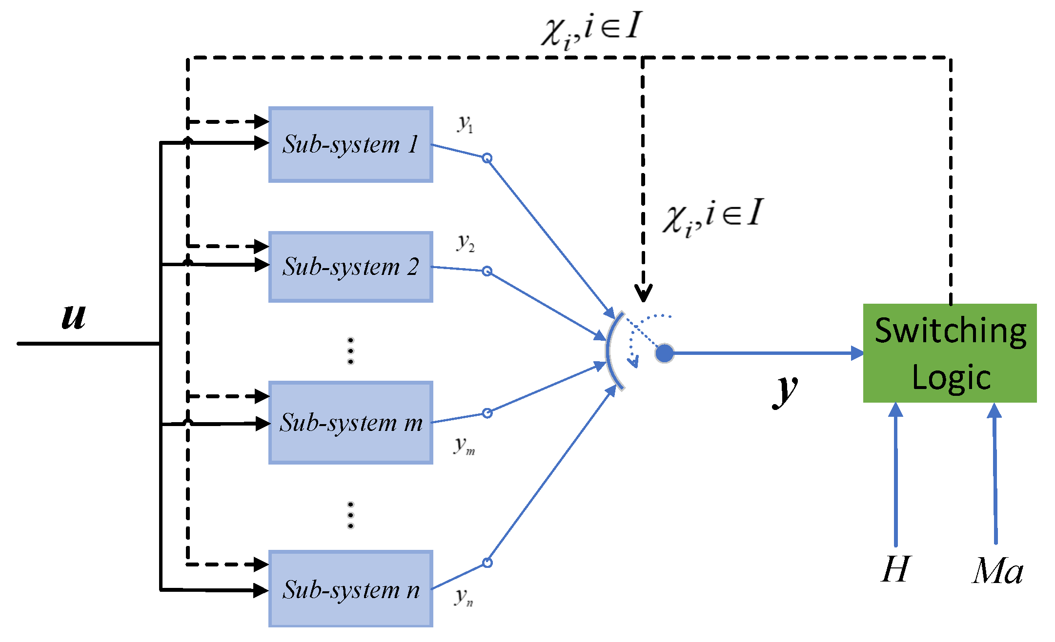
2.1.1. Uncertain Switched System

The uncertain switched system structure is shown in Figure 1. For each subregion, engine dynamics were described by a subsystem like the one shown in Equation (5). Therefore, the nonlinear system (1) can be approximated by the uncertain switched system. It should also be noted that each subregion has a deterministic boundary, which means that there is no intersection between the adjacent subregions.
To simplify the switched system formulation, the notation χ i ( t ) , i I is introduced. In the engine operation, the current operating state and flight conditions determine whether the subsystem is active or not. When the system trajectory enters the subregion X i , the i-th subsystem will be activated and χ i ( t ) will be equal to 1. In the opposite case, the subsystem will be deactivated and χ i ( t ) will be equal to 0, meaning that the subsystem state can be determined by the following indicator function:
χ i ( t ) = 1 , x X i 0 , o t h e r w i s e
The common boundary between the two adjacent subregions is merged into one of them, i.e., i = 1 L χ i ( t ) = 1 , allowing the uncertain switched system to describe the nonlinear system dynamic (1) as:
x ˙ = A x + B u + ξ σ ( x ) + f σ ( x )
where A = i = 1 l A i · χ i ( t ) , B = i = 1 l B i · χ i ( t ) , ξ a ( x ) = i = 1 l ξ a , i ( x ) · χ i ( t ) , and f a ( x ) = i = 1 l f a , i ( x ) · χ i ( t ) .
For each subsystem, a controller was designed aiming to achieve the control performance. Furthermore, all the controllers can be combined into a super controller able to regulate the engine speed within the full operating envelope. Figure 2 shows the control structure of the uncertain switched system.
To describe the switched system evolution, the following switching sequence is provided:
E = l 0 , t 0 , , l i , t i , l i + 1 , t i + 1 , l e , t e , t i R + , l i I Z +
where t i denotes the switching time and l i indicates that the l i -th subsystem is activated. The term ( l i , t i ) suggests that the system evolves according to equation x ˙ = A l i x + B l i u + ξ a , l i ( x ) + f a , l i ( x ) over t [ t i , t i + 1 ) ] , meaning that the equality χ i ( t ) = 1 holds for t i t < t i + 1 . Moreover, E ( j ) = { [ t j 1 , t j 1 + 1 ) , [ t j 2 , t j 2 + 1 ) , , [ t j m , t j m + 1 ) } denotes all the time intervals during which the j-th subsystem is switched on. Finally, sequences E and E ( j ) are not infinite.

2.1.2. Error-Tracking Dynamic System

The error tracking dynamic system was derived to solve the switched system tracking problem. Assuming that r denotes the desired trajectory and e = x r is the tracking error, the error tracking dynamics can be expressed as:
e ˙ = Ax Ar + Ar + B u + ξ a ( x ) + f a ( x ) = Ae + B u + ξ a ( x ) + f a ( x ) + Ar
The last term on the right can be treated as disturbance and thus compensated by the control law [26]. Hence, the derivation will utilize the following error tracking dynamic system:
e ˙ = Ae + B u + ξ σ ( x ) + f σ ( x )
The progression of the error tracking dynamic still follows the partition of X i . Finally, Equation (9) can be expressed as:
e ˙ = Ae + B u + ξ σ ( e ) + f σ ( e )
where ξ σ ( e ) = i = 1 l ξ σ , i ( e ) · χ i ( t ) , and f σ ( e ) = i = 1 l f σ , i ( e ) · χ i ( t ) represent the uncertainties residing in the control input and system dynamics, respectively.
Therefore, the objective is to derive the ISMC control law and design the bumpless transfer scheme for the uncertain switched system. Within the resulting scheme, the tracking error e ( t ) will exponentially converge to the ball centered at the origin. To simplify the controller design, the following assumptions can be made regarding the uncertainties:
Assumption 1.
The uncertainty ξ σ , i ( e ) , i I satisfies ξ σ , i ( e ) h i , 1 e + h i , 2 , where h i , 1 , h i , 2 R + .
Assumption 2.
The uncertainty f σ , i ( e ) , i I satisfies f σ , i ( e ) d i , 1 e , where d i , 1 R + .
The engine time response near the idle can be much different from the response near the maximum rotational speed [1]. It should be noted that the response varies with flight conditions, but this difference is not infinite. Hence, it is implied that the uncertainty term ξ σ , i ( e ) , f σ , i ( e ) boundness is reasonable.
Before concluding the section, the definition and lemma constituting the necessary theoretical foundation for the global stability analysis of the switched closed-loop system are presented.
The definition of average dwell time for switched systems is as follows:
Definition 1.
([22]). Let N σ ( t 1 , t 2 ) denote the number of switching of the switched system over the interval τ 1 , τ 2 , 0 τ 1 < τ 2 R + . If the inequality N σ t 1 , t 2 N 0 + t 2 t 1 / τ d holds for τ d > 0 , 0 N 0 Z , then τ d is denoted as the average dwell time.
Lemma 1.
Consider a switched system z ˙ = A m z , where z R n , A m = A m , i · χ i ( t ) . The Lyapunov function for each subsystem is V i ( t ) = z T P m , i z . For the switching time, there exists a positive constant μ such as:
V k 1 ( t k ) μ · V k ( t k )
where μ = max λ m a x P k 1 / λ min P k .
Proof. 
Consider the switching at a time instant t k . For the k-th switched system subsystem z ˙ = A m z over [ t k , t k + 1 ) , we have:
λ m i n P m , k · z 2 V k ( t ) λ max P m , k · z 2
A lower bound for the Lyapunov function is defined as:
z 2 1 λ m i n P m , k · V k ( t )
where λ m i n · , λ max · denote the minimum and maximum matrix eigenvalues, respectively. For the ( k 1 ) -th subsystem over [ t k 1 , t k ) , the following expression can be written:
λ m i n P m , k 1 · z 2 V k 1 ( t ) λ max P m , k 1 · z 2
At the switching time t k , it is possible to derive:
V k 1 ( t k ) λ max P m , k 1 λ m i n P m , k · V k ( t k ) μ · V k ( t )

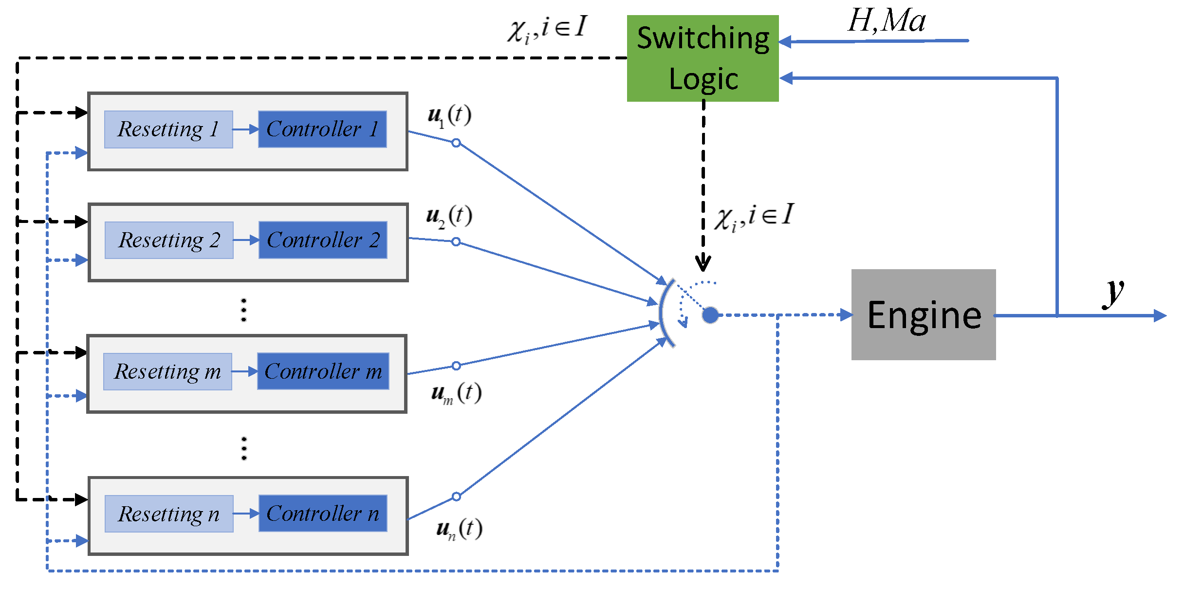
2.2. Controller Design

2.2.1. Integral Sliding Surface

Given the i-th switched system subsystem (10), the integral sliding surface is designed as follows:
s = G i e 0 t G i · ( A i + B i K i ) e d τ
where G i and K i are parameter matrices to be designed. The matrix G i should be selected to ensure that G i B i is non-singular, while the K i will be designed later.
Given the sliding surface (11), the equivalent control law can be derived as:
u e q u = Ke G i B 1 · G i · f σ , i ( e ) ξ σ , i ( e )
By substituting the equivalent control (12) into the system (9), the following sliding motion equation is obtained:
e ˙ = A i + B i K i e + I B G i B −1 G i f σ , i ( e )
The following theorem provides a sufficient condition for the sliding motion equation stability (13).
Lemma 2.
Considering the sliding motion Equation (13), if there exist positive and definite matrices P 1 , i R m × n and W i R m × n , such that the following matrix inequality (14) holds, then the sliding motion Equation (10) is stable, and the parameter matrix K i can be designed as K i = W i P 1 , i −1 .
P 1 A + Q T B T + A P 1 + BQ + I P 1 G ¯ i T G ¯ i P 1 1 / l 2 · I < 0
where G ¯ i = I B G i B −1 G i .
Proof. 
Consider the Lyapunov function candidate V i ( t ) = e T P i e . The time derivative of the Lyapunov function can be written as:
V ˙ i ( t ) 2 e T ( A i + B i K i ) T P i e + e T P i T P i e + f σ , i T ( e ) G ¯ i T G ¯ i · f σ , i ( e )
By applying basic inequalities and the Lipschitz continuity condition f σ , i ( x ) , the following expression is obtained:
V ˙ i ( t ) e T ( A i + B i K i ) T P i + P i ( A i + B i K i ) + P i T P i + l 2 · G ¯ i T G ¯ i · e
This expression is, by algebraic transformation and Schur’s complement, equivalent to the linear matrix inequality (14). Finally, with the inequalities (14), it is trivial to prove that the sliding motion Equation (11) is stable. □

2.2.2. ISMC Control Law for Uncertain Switched System

Based on the aforementioned analysis, the control law (17) can be designed. The following theorem presents the designed method effectiveness for the ISMC control law. Moreover, the system trajectories whose initial state are located at any point can reach the sliding surface in finite time.
Theorem 1.
Consider the uncertain switched system (10) subject to Assumptions 1 and 2. Let the uncertain switched system be controlled by the control law (17). Then, the error tracking system trajectory can reach the sliding surface in finite time.
u i = K i e + u 1 , i u 1 , i = k 1 , i · h 1 , i e + h 2 , i + k 2 , i · d 1 , i e + d 2 , i + i · s g n ( s )
where k 1 , i = ( G i B i ) 1 · G i B i , k 2 , i = ( G i B i ) 1 · G i , and ϵ i > 0 .
Proof. 
When the i-th subsystem is activated, consider the following Lyapunov function candidate:
V 1 , i ( t ) = 1 2 s T ( G i B i ) 1 s
the time derivative of which is given by:
V ˙ 1 , i ( t ) = s T · ξ σ , i ( e ) + s T ( G i B i ) 1 · G i f σ , i ( e ) + s T u s T K i e
According to Assumptions 1 and 2, we have:
V ˙ 1 , i ( t ) s ( G i B i ) −1 · G i B i · h 1 , i · e + h 2 , i + G i · d 1 , i · e + d 2 , i + s T u 1
By substituting the control law (17) into (19), one obtains:
V ˙ 1 , i ( t ) ϵ · s ( t )
As can be seen, Equation (20) implies that the trajectories of the state will be driven to the specified sliding surface. Next, it is necessary to prove that the system state will reach the sliding mode surface in a finite time. An upper Lyapunov function bound is given as:
V 1 , i ( t ) 1 2 λ m a x ( G i B i ) · s ( t ) 2
Combined with (20) and (21), it is possible to derive:
V ˙ 1 , i ( t ) ϵ i · 2 / λ m a x G i B i 1 · V 1 , i ( t )
By utilizing the basic equality that V i ( t e ) = 0 , where t e denotes the time when the system trajectory reaches the sliding surface. After integrating both sides of Equation (22), we have:
Δ T ϵ i · V 1 , i ( t 0 ) 2 / λ m a x G i B i 1
where Δ T = t e t 0 denotes the time needed to reach the sliding surface. Combined with (21), one can obtain that:
Δ T ϵ 2 · λ m a x ( G i B i ) −1 · s ( t 0 )
It is obvious that the tracking error e ( t ) will reach the sliding mode surface in finite time. Additionally, the length of time interval Δ T can be adjusted through the selection of ϵ i and s ( t 0 ) . □

2.3. Bumpless Transfer Scheme

A sliding surface resetting scheme was designed to achieve the bumpless transfer between neighboring controllers. In this scheme, when switching the j-th sub-controller to the i-th one, the initial value of the i-th sub-controller sliding surface will be reset to minimize the objective function in Equation (24). Hence, the resetting scheme can be converted into the optimization problem:
s i ( t i ) = arg min u i ( t i ) u j ( t i ) , i , j I
where u i ( · ) , u j ( · ) are the control input signal generated by the i-th and j-th sub-controller, respectively, s i ( t i ) is the initial value of the i-th sub-controllers sliding surface, and t i denotes the moment prior to time t i .
The scheme is proposed to ensure the control input continuity during controller switching by resetting the initial state of sliding surface. To achieve this task, sigmoid-like functions are introduced to replace the sign function. With the resetting scheme, input continuity can be ensured, which means that the system trajectory can directly enter another subregion without system output variables oscillation.

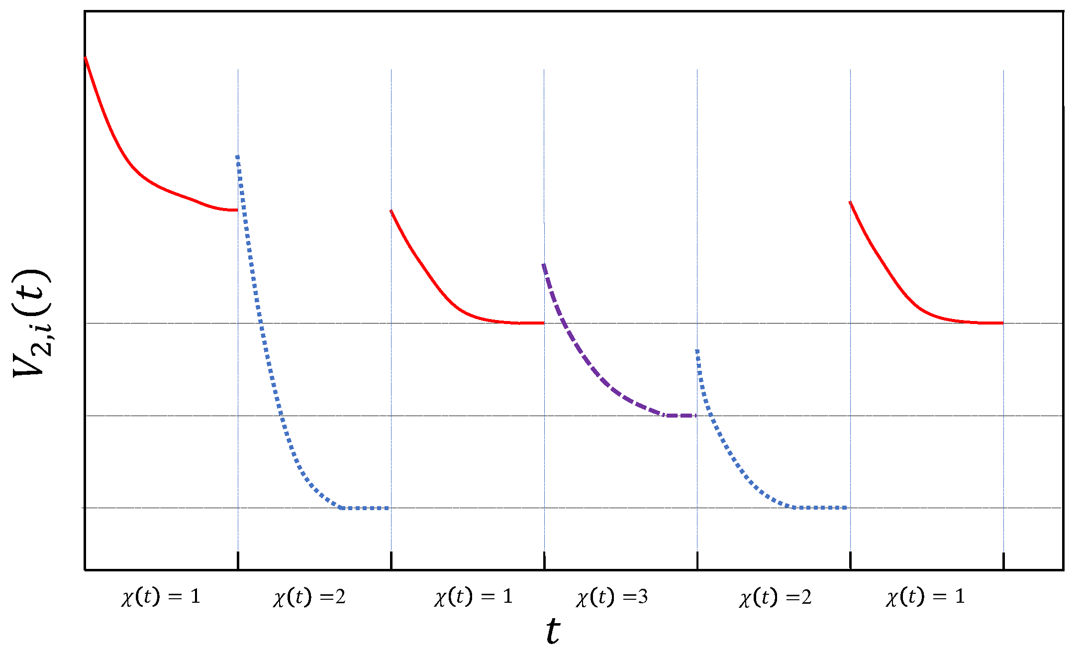
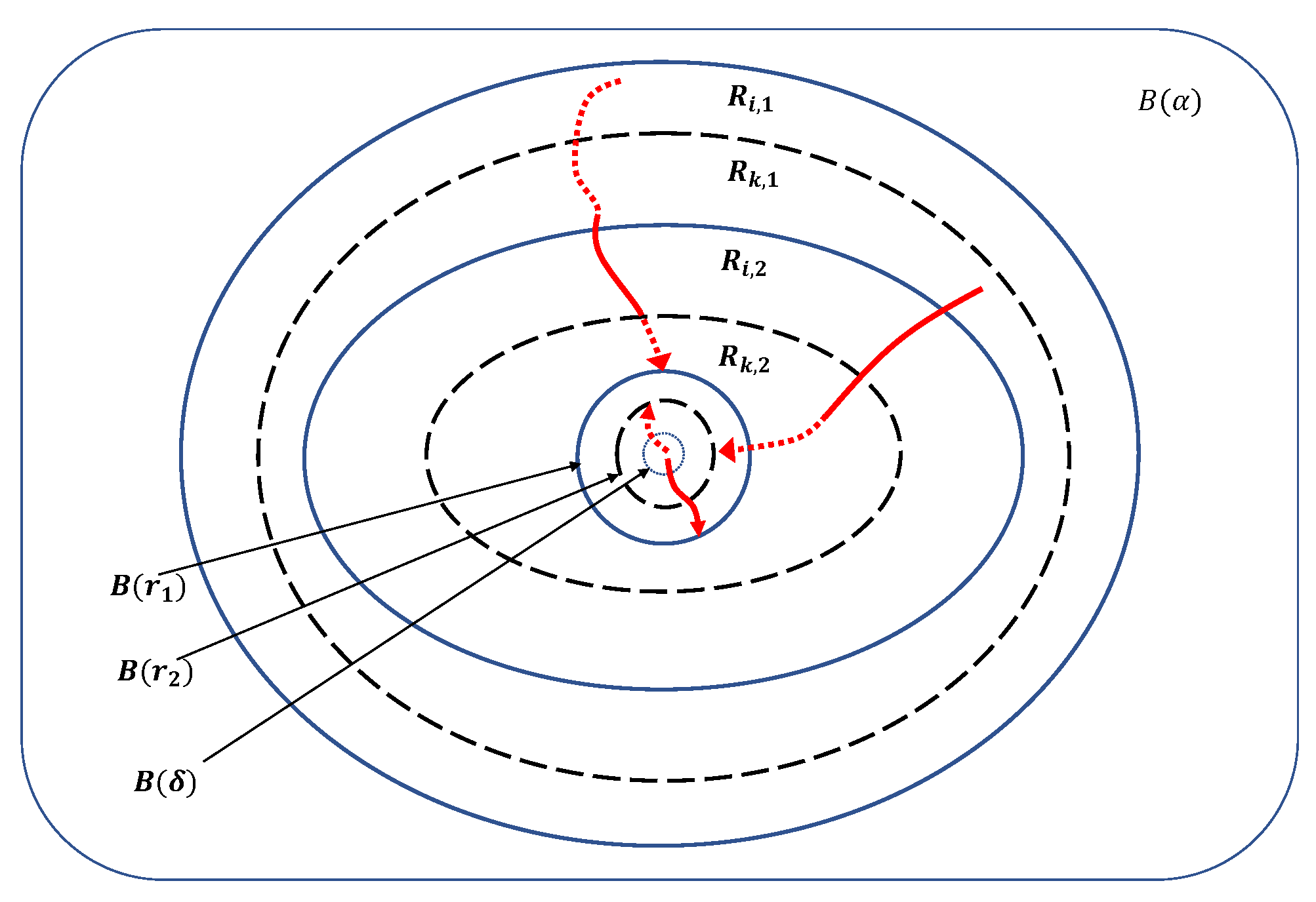
2.4. Global Stability of the Uncertain Switched System

When t [ t i , t i + 1 ) , the i-th subsystem is active and χ i ( t ) = 1 . By substituting the designed controller (17) into (10), the closed-loop subsystem is found as:
e ˙ = ( A i + B i K i ) e + B i u 1 , i + B i ξ σ , i ( e ) + f σ , i ( e )
The system can be rewritten as:
e ˙ = A a , i e + B i u 1 , i + B i · ξ σ , i ( e ) + f σ , i ( e )
where A a , i = A i + B i K i .
With the parameter matrix K i , i I in Theorem 1, the following theorem presents the global stability and tracking properties of the switched closed-loop system.
Theorem 2.
Consider the closed-loop system consisting of the uncertain switched system (10) and the controller (17) with the sliding surface (11). For the given matrix K i which satisfies the inequality (14), if there is a positive and definite matrix P 2 , i and matrix Q i such that the inequality (27) holds, the closed-loop system (26) is stable.
Γ i = Φ i B i T P 2 , i P 2 , i B i β 1 · I < Q
where Φ i = A i + B i K i T P 2 , i + P 2 , i A i + B i K i + β P 2 , i + 2 l · P 2 , i + 2 h i · B T P 2 , i .
Proof. 
Considering the Lyapunov candidate V 2 , i ( t ) = e T P 2 , i e , the derivative of which is:
V ˙ 2 , i ( t ) = e T ( A a , i T P 2 , i + P 2 , i A a ) e + 2 u 1 , i T B T P 2 , i e + 2 f σ T ( e ) P 2 , i e + 2 ξ i T ( e ) B P 2 , i e
Define the following auxiliary function:
J i ( t ) = V ˙ 2 , i + β V 2 , i + β 1 · u 1 T u 1
By applying Assumptions 1 and 2, Equation (29) can be written as:
J i ( t ) e T A i + B i K i T P 2 , i + P 2 , i A i + B i K i e + β e T P i e + 2 u 1 , i T B T P i e + 2 ξ i T B T P 2 , i e + 2 f i T P 2 , i e + β 1 · u 1 T u 1 e T A i + B i K i T P 2 , i + P 2 , i A i + B i K i + β P 2 , i + 2 h 1 , i B i T P 2 , i + 2 d 1 , i · P 2 , i e + 2 u 1 , i T B T P i e + β 1 · u 1 T u 1 β 1 · u 1 T u 1 + 2 h 2 , i B i T P 2 , i e + 2 d 2 , i P 2 , i e
Using the Schur complementary and the inequality (25), we write:
J i ( t ) ζ i T Q ζ β 1 · u 1 T u 1 + 2 h 2 , i B i T P 2 , i e + 2 d 2 , i P 2 , i e
where
Γ i = A i + B i K i T P 2 , i + P 2 , i A i + B i K i + β P 2 , i + 2 l P 2 , i + 2 h i B i T P 2 , i B i P 2 , i P 1 2 , i B i β 1 I
ζ = [ e , u 1 ] T
Let r i = 2 ( 1 + k ) / ( 1 + α ) · h 2 , i B i P 2 , i + d 2 , i P i / λ m i n Q i , where 1 < α < 2 , 0 < k R , and define the Ball B ( r i ) = e e r i . When e ( t ) R n / B ( r i ) , we have
J i ( t ) ( 1 + α ) · ζ T Q i ζ + 2 h 2 , i B i T P i + d 2 , i P 2 , i · e η i · e 2
where η i = ( 1 + α ) · k / ( 1 + k ) · λ m i n Q i . Thus, it can be observed that:
V ˙ 2 , i ( t ) β · V 2 , i ( t )
Integrating the above presented equation yields:
V 2 , i ( t ) V 2 , i ( t i ) · e β · ( t t i )
When e ( t ) B ( r i ) , one obtains:
V 2 ( t ) v i
where v i = λ m a x P 2 , i · r i 2 .
Finally, this can be summarized as:
V 2 ( t ) V 2 ( t i ) · e β · ( t t i ) , e > r i λ m a x P 2 , i · r i 2 , e r i
Once the system trajectory enters B ( r i ) , it stays in the ball. Therefore, V 2 ( t ) max λ m a x P 2 , i r i 2 , V 2 ( t i ) , and the closed-loop system stability can be confirmed. In each subregion X i , the system trajectory exponentially converges to a relatively small neighborhood around the origin.
In the complete engine operation process, the system trajectory will pass through a series of subregions, and two cases might happen. Firstly, the system trajectory can enter into balls in multiple subregions, but has not passed through all the subregions (Case 1), i.e., e B ( r i ) , i I . The second possibility is that in each subregion, the system trajectory will always be outside of the ball (Case 2), i.e., e B ( r i ) , i I . In the following paragraphs, we will prove that the tracking error can enter into a boundary layer region, regardless of the case.
Case 1: e B ( r i ) , i I
In this case, the system trajectory enters into the balls in multiple subregions, i.e., V 2 ( t ) λ m a x P 2 , i · r i 2 occurs in multiple elements E during the entire control process. We will show the stability of the origin in the sense of Lyapunov.
According to Equations (33) and (34), it can be concluded that the system trajectory starts at the ball B ( r j ) , j I and stays within it for any t > t 0 . The system trajectory starts in R n / B ( r j ) and converges exponentially faster B ( r j ) . The system trajectory enters the ball B ( r i ) , which can be described as V 2 ( t ) v i . Finally, Figure 3 depicts the history of multiple subsystems’ Lyapunov functions over time for l = 3.
Consider the ball B ( α ) = e : e α of radius α > 0 around the origin, and define the set R m = e : V 2 ( t ) c m , c m > 0 in B ( α ) . When χ j ( t ) = 1 , the set for the z-th element of E ( j ) is defined as R j , z = e : V 2 , j ( t ) c j , z , c j , z > 0 . For each element in the sequence E ( · ) , a set similar to R m was constructed. Moreover, the set R j , z + 1 is contained in R j , z , and all the sets can be denoted as R j , · . According to Equation (34), it can be obtained that r j c j . Similarly, a series of sets R k , · , k I can be defined for the series E ( k ) , and all these sets are contained in B ( α ) . More details can be seen in Figure 4 (for l = 2).
Denoted by δ , the ball radius around the origin lies in the intersection of all the nested set sequences R j , · , j I . According to Equations (33) and (34), it can be found that these sets have the property that any trajectory starting in B ( r j ) at t 0 stays in B ( r j ) , j I for all t > t 0 , and that the trajectory starting in B ( α ) / B ( δ ) at t 0 stays in B ( α ) for all t > t 0 . Furthermore, if the dwell time of the j-th subsystem is long enough, which means that the system trajectory converges to B ( r j ) , j I at the end [16]. Figure 4 depicts the system trajectory over time (l = 2).
Case 2: e B ( r i ) , i I
In this case, the system trajectory is always outside of balls, with the last subregion being the exception, i.e., B ( r i ) , i I , in each element E over t [ t 0 , t e n d ) , where t 0 , t e n d are initial and end times of the control process, respectively. It can be concluded that the tracking errors are exponentially convergent.
According to Lemma 1 and Equation (33), when the i-th subsystem is active, for any t [ t i , t i + 1 ) , we can obtain:
V 2 , i ( t ) μ · V 2 , i 1 ( t i ) · e β · ( t t i )
By using the iterative method, it is derived that:
V 2 , i ( t ) V 2 , i ( t i 1 ) · e β · ( t t i ) μ · V 2 , i 1 ( t i ) · e β · ( t t i ) μ · V 2 , i 1 ( t i 2 ) · e β · ( t t i 1 ) μ 2 · V 2 , i 2 ( t i 2 ) · e β · ( t t i 1 ) μ 2 N σ ( t 0 , t ) 1 · V 2 , 1 ( t 0 ) · e β · ( t t 0 ) μ 1 · e 2 N σ ( t 0 , t ) · ln μ β ( t t 0 ) · V 2 ( t 0 )
Due to the fact that N σ ( t 0 , t ) N 0 + ( t t 0 ) / τ d and N 0 = 0 , Equation (36) can be rewritten as:
V 2 , i ( t ) μ 1 · e 2 N σ ( t 0 , t ) · ln μ β ( t t 0 ) · V 2 , 1 ( t 0 )
Finally, it can easily be concluded that:
e ( t ) ρ ρ μ μ · e ( t t 0 ) / τ d · ln μ 1 2 β ( t t 0 ) · x ( t 0 )
where ρ = λ m i n ( P 2 , 1 ) λ m i n ( P 2 , 1 ) λ max ( P 2 , i ) λ max ( P 2 , i ) .
It can be concluded that if the average dwell time τ d satisfies the bound τ d 2 ln μ / β , the Lyapunov function V 2 , i ( t ) converges to the ball B ( r i ) exponentially as t . This allows for the upper tracking error bound to be determined, which proves the global asymptotic stability of the switched closed-loop system. □

3. Numerical Simulation

In this section, an uncertain switched system describing the engine dynamics was used to illustrate both the applicability and effectiveness of the proposed control method with the resetting scheme. The maximum fan and core speeds of the high bypass ratio turbofan engine were N 1 = 3390 rpm and N 2 = 10,300 rpm, respectively. The component level engine model used in the simulations was based on the Toolbox for the Modeling and Analysis of Thermodynamic Systems (T-MATS) [26]. Moreover, all the engine performance maps and relevant component data were acquired from the Gas Turbine Simulation Program (GSP) [29]. In the nonlinear model, N 1 and N 2 were selected as the state variables, while the fuel flow was regarded as the control input. Moreover, the thrust was controlled indirectly by controlling N1 according to the turbofan engine control practice.
The allowable operating range of the engine should be partitioned based on the operating conditions and operating state of the engine when aiming to describe the engine dynamics using an uncertain switched system. As the first step of operating range partitioning, the flight envelope is divided into several zones. Additionally, the generalized distance d in Equation (38) is defined to evaluate the level of similarity between the two different flight points located on the envelope.
d = P 1 P 1 k P 1 k 2 + T 1 T 1 k T 1 k 2 + V 0 V 0 k V 0 k 2
where P 1 k , T 1 k , and V 0 k are inlet total pressure, inlet total temperature, and flight speed of the k-th zone’s nominal point, respectively; P 1 , T 1 , and V 0 are the inlet total pressure, inlet total temperature, and flight speed of a specified point, respectively. These variables can be calculated by flight altitude H and Mach number M a .
The flight envelope division can be transformed into a minimax problem. This type of optimization problem aims to cover the full flight envelope using the minimum number of zones and the least generalized distance. The optimization problem can be formalized as:
max α k k = 1 s min d ¯ k k = 1 s F ( α 1 , , α s , d ¯ 1 , , d ¯ s ) s . t . k = 1 s α k 1
where s Z + is the number of zones, d ¯ k , k = 1 , 2 , , s is the upper limit of the generalized distances for the point in the k-th zone, α k denotes the k-th zone coverage, and F ( · ) R is the objective function, denoting the sum of all the zone coverages.
To reduce the computational complexity, the optimization method can be replaced by a clustering algorithm. Using the k-means clustering algorithm, all points in the flight envelope surrounding the flight profile are divided into several zones. The simulations with five, seven and nine zones have similar results, yet the scenario with seven or nine zones has more subsystems and nominal points to be listed. For concise illustration, five zones are selected to conduct the simulation, and the division results are shown in Figure 5. Based on these zones, the allowable operating range X is partitioned into seven subregions, and the nominal points of these subregions X i X , i I = 1 , 2 , , 7 are shown in Table 1. The switching rule of the switched system is also determined by these subregions.
In each subregion, a subsystem as Equation (5) can be obtained to describe the engine dynamics. All the subsystems can be written as:
Subsystem 1:
x ˙ = −6.1820 0.9154 −2.5747 −0.7385 · x + 3037.1 2108.6 · u + ξ 1 + f σ , 1 ( x )
Subsystem 2:
x ˙ = −6.7006 1.0100 −0.0494 −0.4852 · x + 4293.7 2913.4 · u + ξ 2 + f σ , 2 ( x )
Subsystem 3:
x ˙ = −5.1625 1.0785 −0.0249 0.4830 · x + 4113.3 2980.5 · u + ξ 3 + f σ , 3 ( x )
Subsystem 4:
x ˙ = −6.6661 0.8405 −2.3136 0.7008 · x + 3132.3 2143.2 · u + ξ 4 + f σ , 4 ( x )
Subsystem 5:
x ˙ = −6.4694 0.8804 −1.4859 1.4068 · x + 2738 2238.6 · u + ξ 5 + f σ , 5 ( x )
Subsystem 6:
x ˙ = −4.5487 0.5715 −1.1611 0.4838 · x + 3.0257 2.2439 · u + ξ 6 + f σ , 6 ( x )
Subsystem 7:
x ˙ = −3.7100 0.4914 −0.8889 0.7592 · x + 2.9036 2.4122 · u + ξ 7 + f σ , 7 ( x )
All these subsystems and the corresponding switching rules constitute the uncertain switched system as shown in Figure 1. In the controller design, the following parameter values were selected: G = 1.891 × 10 4 1.242 × 10 4 , h 1 , i = 2.13 × 10 3 , h 2 , i = 3.4 × 10 2 , d 1 , i = 3.2 , i = 1 , , 7 to bound the system uncertainties in system dynamics. The YALMIP [30] was used as the LMI solver to find suitable matrices K i , i = 1 , , 7 . Finally, the control structure as shown in Figure 2 was built for simulation.

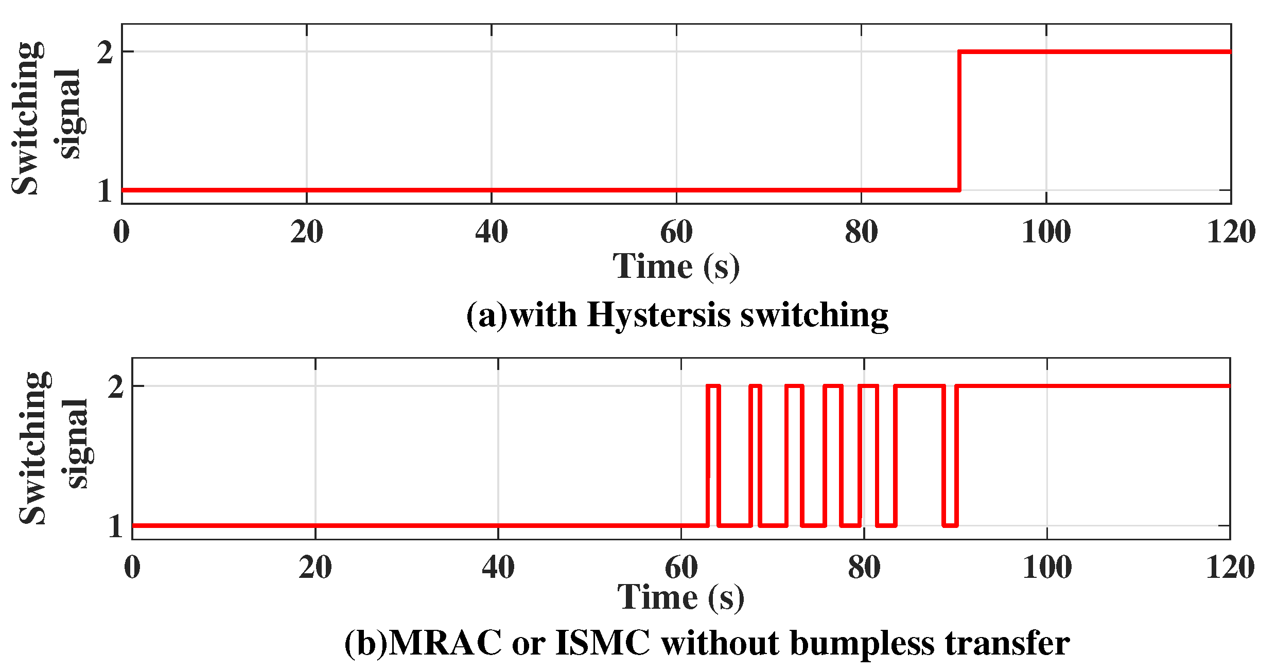
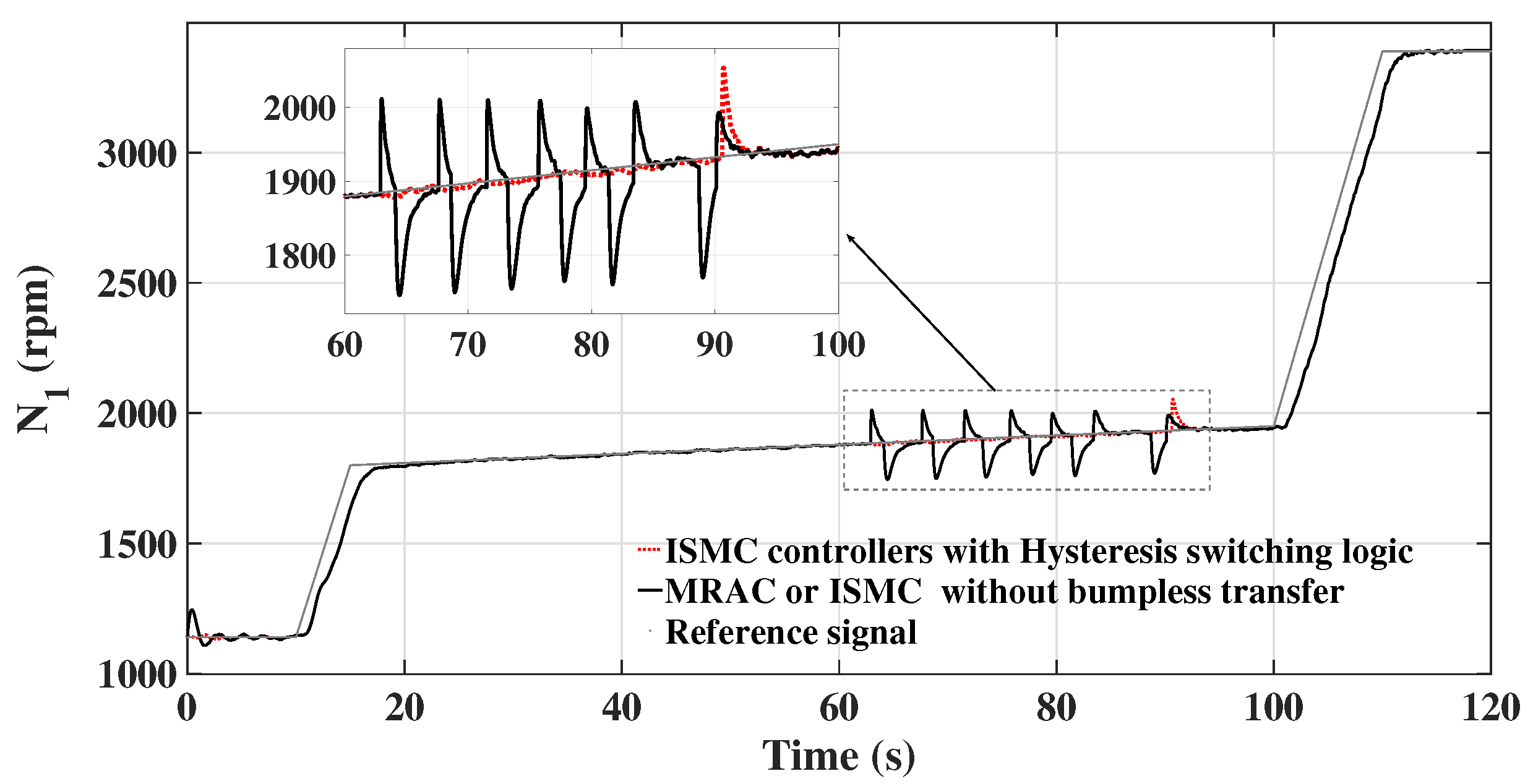
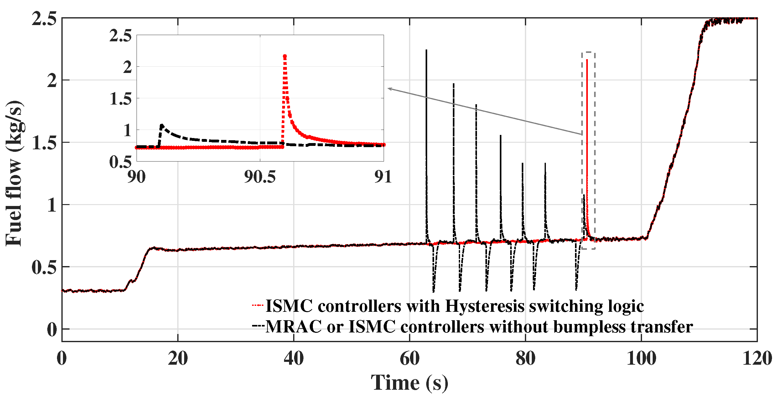
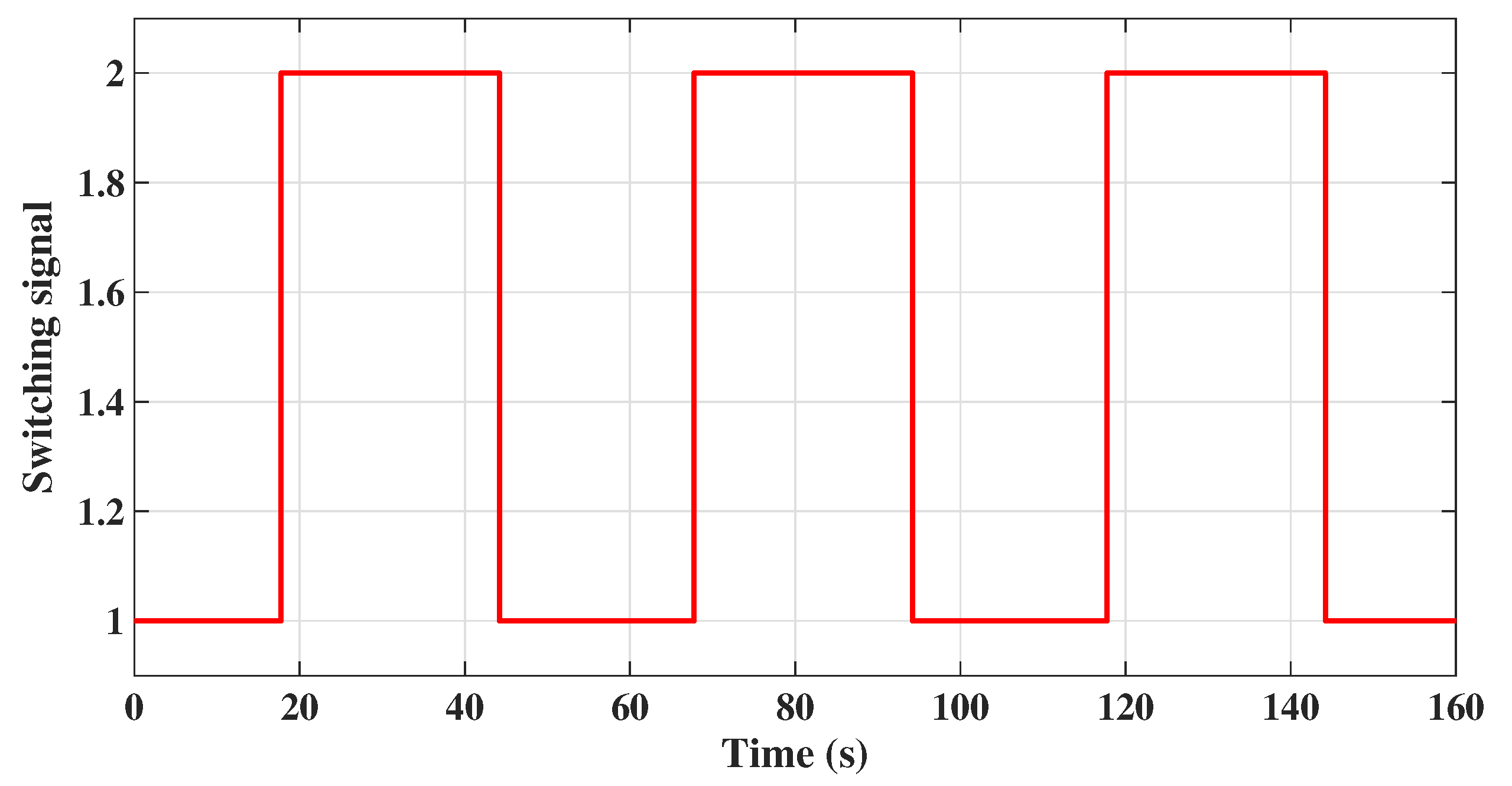
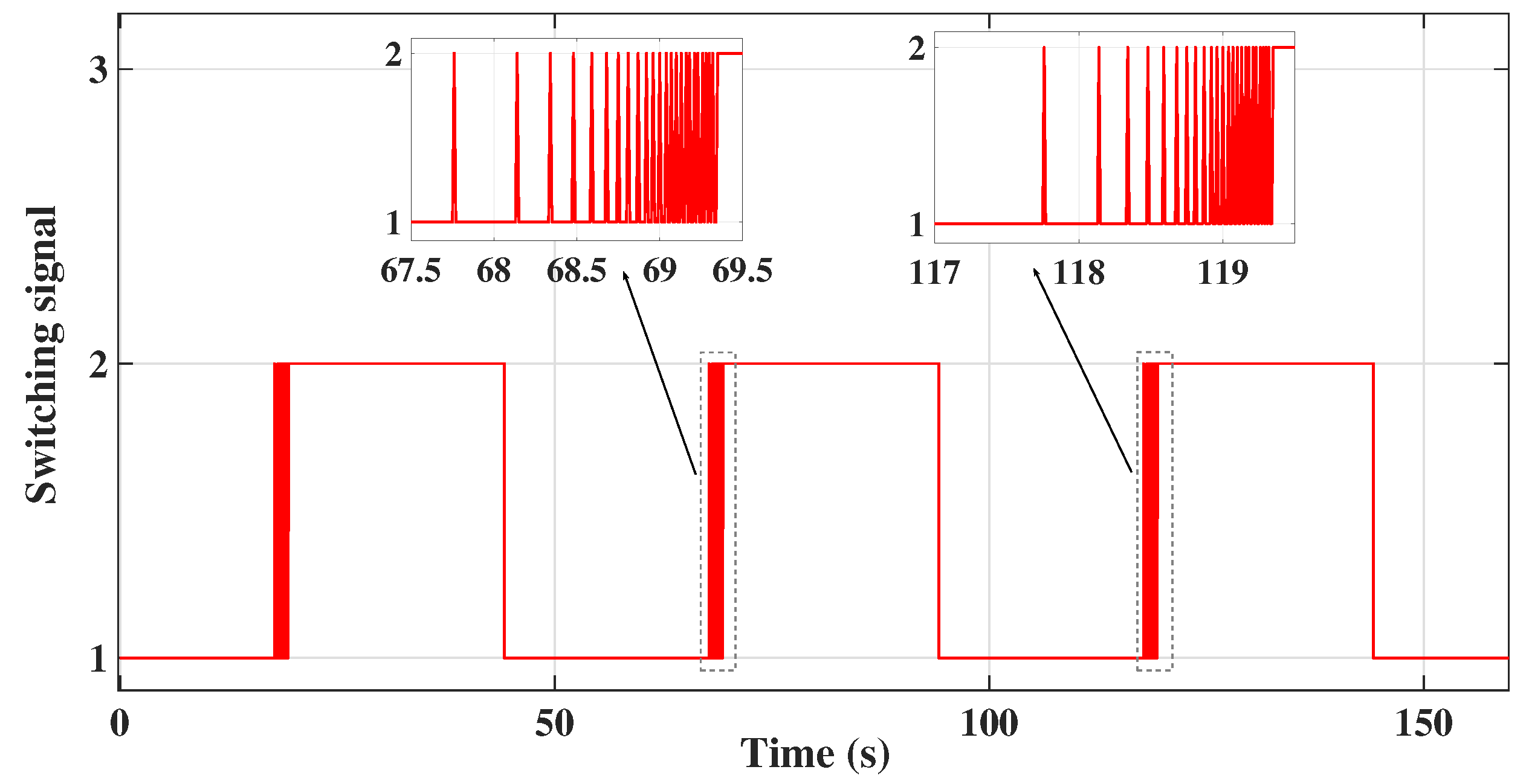
3.1. The Importance of Bumpless Transfer

The control objective is to drive the Fan speed N1 to track the reference signal by regulating the fuel flow. To illustrate the importance of bumpless transfer between two controllers, a comparative simulation with two subsystems was performed. The operation condition was set as H = 0, M a = 0, and Subsystem 1 and Subsystem 2 were included in the simulation. The partitioned subregions were X 1 = { x : [ 1140 , 5828.8 ] T x < [ 1900 , 7191.4 ] T } , X 2 = { x : [ 1900 , 7191.4 ] T x [ 3390 , 10,314.2 ] T } . Additionally, the operating range starting from idle to maximum speed was covered.
According to Theorem 1, the feedback matrix K i can be obtained by solving the LMI in (14).
K 1 = [ 0.01276 , −0.02489 ] , K 2 = [ 0.51303 × 10 3 , 0.48426 × 10 3 ]
In the simulation, a sigmoid-like function s ( t ) / ( | s ( t ) | + c ) , c = 0.008 was introduced to replace the sign function.
Given the adverse effects of the noise and disturbance, the results are compared in Figure 6, Figure 7 and Figure 8. In the comparison simulation of the MRAC scheme, the parameter freezing method was included into the control structure to ensure the continuity of control input. However, the system oscillation and high-frequency controller switching during the controller transition process can still be observed. This phenomenon is similar to the ISMC method and some other control schemes without bumpless transfer mechanism. Hence, only one simulation result was displayed in Figure 6, Figure 7 and Figure 8.
The switching signals for various cases are shown in Figure 6. The frequent switching phenomenon between the neighboring controllers can be seen in Figure 6b. Figure 7 and Figure 8 show the tracking errors and fuel flows for the controller transition of various control methods. The transient behaviors caused by controller switching are shown in the detail views of Figure 7 and Figure 8. As can be seen from the detail views in Figure 7, the traditional switching method cannot ensure input continuity, and abrupt change of control input can be seen.
Hysteresis switching logic can avoid the high-frequency switching occurring, but it cannot ensure the control input continuity. The output discontinuity caused by hysteresis switching logic is shown in Figure 7. The output oscillations caused by controller transition without bumpless transfer mechanism are also shown in Figure 7.
Finally, it can be concluded that controller switching will cause undesired transient behaviors, significantly degrading the system performance. Therefore, it is necessary to introduce the bumpless transfer mechanism for controller transition.

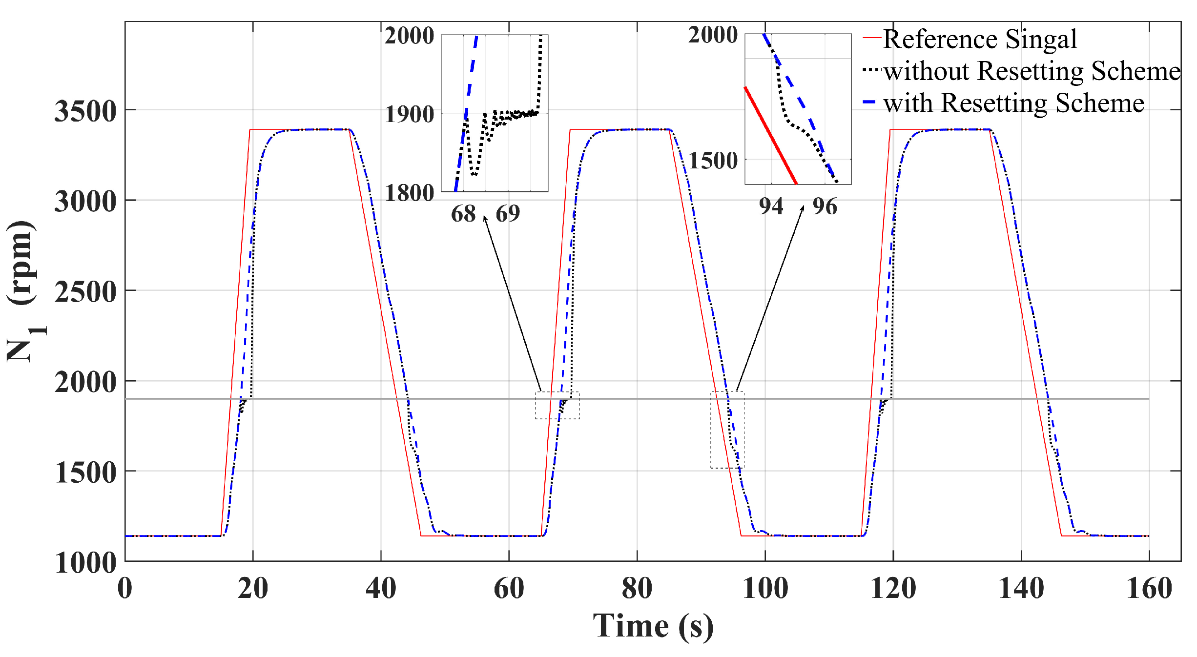
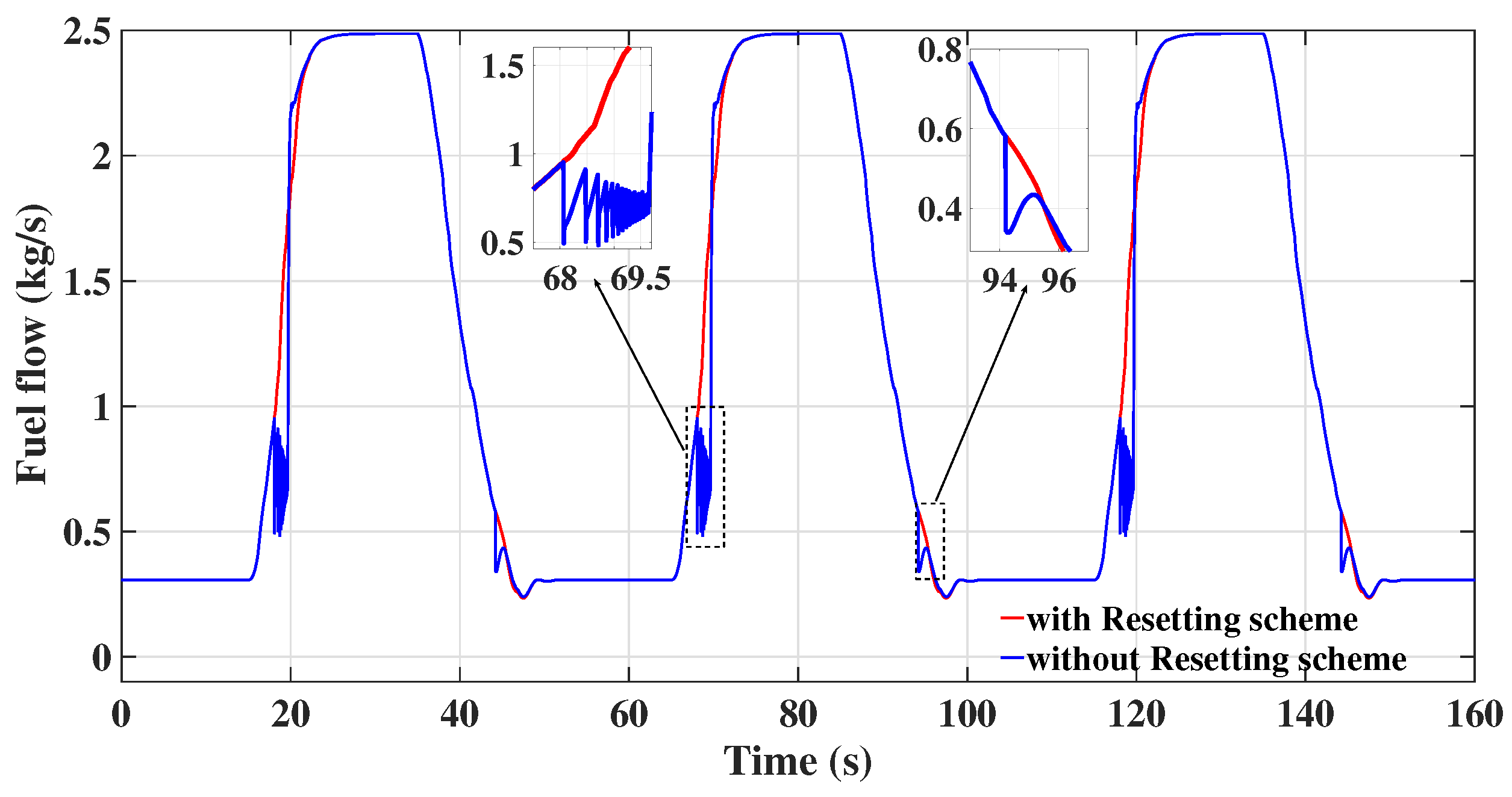
3.2. The Resetting Scheme Effectiveness

A comparative simulation was carried out to demonstrate the resetting scheme effectiveness in regards to the controller switching. Subsystem 1, Subsystem 2, and corresponding ISMC controllers were included in the simulation. Figure 9 and Figure 10 show the ISMC controller switching signals with and without resetting scheme, respectively, while Figure 11 shows the N1 history (the grey line corresponds to the switching event). In this simulation, the engine accelerates to the maximum speed in 4.97 s with almost no overshoot, and the system trajectories can simply cross the boundaries. This cannot be achieved by controllers without the resetting scheme.
The fuel flows are shown in Figure 12. It can be seen that controller transition without the resetting scheme can cause a significant control input discontinuity. As a result, the high-frequency switching phenomenon can occur. Such results suggest that the resetting scheme can help effectively avoid the input discontinuity during the controller switching.

3.3. The Robustness and Effectiveness of the ISMC Control Scheme

The complete engine operation within the flight envelope, including takeoff, climb, level flight, cruise, and descent was simulated to verify the ISMC method effectiveness. The flight profile is shown in Figure 6. During the take-off and climb phases, the engine was operating at the maximum speed, while in the cruise phase, it was operating at 85% maximum speed. During the descent, the engine was operating at approximately 50% of the maximum speed, which was gradually reduced to 30% as H and M a decreased. Finally, all seven subsystems were included in the simulation. The control objective was to obtain the fan speed N 1 to enable tracking the reference signal within the flight envelope.
The switching signals are shown in Figure 13. When the system trajectories enter the i-th subregion, the i-th controller will regulate the fan speed N 1 . In the simulation, χ i ( t ) = 1 and χ i ( t ) = 0 denote whether the i-th controller is active or inactive, respectively. It can be seen that controllers switch at 34.5 s, 103.68 s, 307.61 s, 399.01 s, 517.17 s, 837.86 s, 993.14 s, 1174.22 s, and 1302.37 s. These seven controllers were activated when system trajectories entered the corresponding pre-assigned subregion.
The simulation results for N 1 and the high-pressure rotor speed N 2 are shown in Figure 14, Figure 15 and Figure 16. It is evident that the proposed control method can enforce N 1 to track the reference signal accurately, without the steady error along with the full operating envelope. Furthermore, the fuel flow is shown in Figure 17, and the control input continuities during the controller transition process can be guaranteed by the resetting scheme.
Turbofan engine fan speed N 1 can be regulated by the designed controller to indirectly achieve the thrust control within the full flight envelope. The thrust produced by the engine is shown in Figure 18.

4. Conclusions

To solve the bumpless transfer problem between ISMC controllers of an uncertain switched system, this paper proposed the ISMC controllers with a resetting scheme. Controllers were designed based on the ISMC method and were implemented in a turbofan engine, and the simulation results have shown the effectiveness of the proposed method. Based on the results, the following conclusions are reached:
(1) The bumpless transfer problem can be solved by using the proposed resetting scheme, which was tested on the uncertain switched system describing the turbofan engine dynamics across the flight envelope. After the controller switching, the changes of fuel flow and output variables are less than 0.41 % and 0.21 % , respectively. Therefore, it was shown that the input discontinuities and output variable oscillations caused by controller transition can be avoided.
(2) Given the transient behaviors caused by controller switching, the global stability of the switched closed-loop system was analyzed and verified by the multiple Lyapunov function method and average dwell time conditions.
(3) The ISMC controllers designed in the paper can control the turbofan engine fan speed to track the reference signal very well, which demonstrates the effectiveness of the proposed method. The acceleration time from idle to maximum speed is less than 5 s, and the steady-state error is below 0.02 % . Finally, the controllers have shown strong robustness against system uncertainties. The control performance across a wide operating range can be ensured by one controller with the help of a well-designed desired signal.
(4) However, the control loops of limit protection were not considered in this control structure, which may affect the control system and tracking performance. Hence, limit protection should be considered in further research.
(5) In addition, the redundant system of the controlled plant can be considered to solve system uncertainty, actuator fault, and engine degeneration by introducing extended systems. This will be also addressed in future work.

Author Contributions

Conceptualization, P.S.; data curation, P.S., B.Y.; formal analysis, P.S., B.Y., H.C. and B.W.; funding acquisition, X.W.; investigation, P.S., S.Y. and H.C.; methodology, P.S.; project administration, S.Y.; resources, X.W.; software, S.Y.; supervision, X.W.; validation, P.S., B.Y. and B.W.; visualization, X.W.; writing—original draft, P.S.; writing—review and editing, P.S., X.W., S.Y. and H.C. All authors have read and agreed to the published version of the manuscript.

Funding

This research was funded by the National Science and Technology Major Project (2017-V-0015-0067), and the National Natural Science Foundation of China (No. 51766011).

Institutional Review Board Statement

Not applicable.

Informed Consent Statement

Not applicable.

Data Availability Statement

The data presented in this study are available on request from the corresponding author.

Conflicts of Interest

The authors declare no conflict of interest.

References

  1. Jaw, L.C.; Mattingly, J. Aircraft Engine Controls: Design, System Analysis, and Health Monitoring; AIAA: Reston, VA, USA, 2009. [Google Scholar]
  2. Richter, H. Advanced Control of Turbofan Engines; Springer Science & Business Media: New York, NY, USA, 2011. [Google Scholar]
  3. Gu, N.; Wang, X.; Lin, F. Design of Disturbance Extended State Observer (D-ESO)-Based Constrained Full-State Model Predictive Controller for the Integrated Turbo-Shaft Engine/Rotor System. Energies 2019, 12, 4496. [Google Scholar] [CrossRef] [Green Version]
  4. Bei, Y.; Xi, W.; Penghui, S. Non-affine parameter dependent LPV model and LMI based adaptive control for turbofan engines. Chin. J. Aeronaut. 2019, 32, 585–594. [Google Scholar]
  5. Leith, D.J.; Leithead, W.E. Survey of gain-scheduling analysis and design. Int. J. Control 2000, 73, 1001–1025. [Google Scholar] [CrossRef]
  6. Balas, G.J. Linear, parameter-varying control and its application to a turbofan engine. Int. J. Robust Nonlinear Control-IFAC-Affil. J. 2002, 12, 763–796. [Google Scholar] [CrossRef]
  7. Wolodkin, G.; Balas, G.J.; Garrard, W.L. Application of parameter-dependent robust control synthesis to turbofan engines. J. Guid. Control Dyn. 1999, 22, 833–838. [Google Scholar] [CrossRef]
  8. Liberzon, D.; Morse, A.S. Basic problems in stability and design of switched systems. IEEE Control. Syst. Mag. 1999, 19, 59–70. [Google Scholar]
  9. Niu, B.; Zhao, J. Tracking control for output-constrained nonlinear switched systems with a barrier Lyapunov function. Int. J. Syst. Sci. 2013, 44, 978–985. [Google Scholar] [CrossRef]
  10. Yang, D.; Zong, G.; Karimi, H.R. H Refined Antidisturbance Control of Switched LPV Systems With Application to Aero-Engine. IEEE Trans. Ind. Electron. 2019, 67, 3180–3190. [Google Scholar] [CrossRef]
  11. Liu, M.; Zhang, L.; Shi, P.; Zhao, Y. Sliding mode control of continuous-time Markovian jump systems with digital data transmission. Automatica 2017, 80, 200–209. [Google Scholar] [CrossRef]
  12. Turso, J.; Litt, J. Intelligent, Robust Control of Deteriorated Turbofan Engines via Linear Parameter Varing Quadratic Lyapunov Function Design. In Proceedings of the AIAA 1st Intelligent Systems Technical Conference, Chicago, IL, USA, 20–22 September 2004; p. 6363. [Google Scholar]
  13. Lu, J.; Brown, L.J. A multiple Lyapunov functions approach for stability of switched systems. In 2010 American Control Conference; IEEE: Piscataway, NJ, USA, 2010; pp. 3253–3256. [Google Scholar]
  14. Hespanha, J.P.; Morse, A.S. Stability of switched systems with average dwell-time. In Proceedings of the 38th IEEE Conference on Decision and Control (Cat. No. 99CH36304), Phoenix, AZ, USA, 7–10 December 1999; IEEE: Piscataway, NJ, USA, 1999; Volume 3, pp. 2655–2660. [Google Scholar]
  15. Li, Z.; Soh, C.B.; Xu, X. Lyapunov stability of a class of hybrid dynamic systems. Automatica 2000, 36, 297–302. [Google Scholar] [CrossRef]
  16. Branicky, M.S. Multiple Lyapunov functions and other analysis tools for switched and hybrid systems. IEEE Trans. Autom. Control 1998, 43, 475–482. [Google Scholar] [CrossRef] [Green Version]
  17. Wu, C.; Zhao, J.; Sun, X.M. Adaptive tracking control for uncertain switched systems under asynchronous switching. Int. J. Robust Nonlinear Control 2015, 25, 3457–3477. [Google Scholar] [CrossRef]
  18. Lian, J.; Zhao, J.; Dimirovski, G.M. Integral sliding mode control for a class of uncertain switched nonlinear systems. Eur. J. Control 2010, 16, 16–22. [Google Scholar] [CrossRef]
  19. Zhao, H.; Niu, Y. Finite-time sliding mode control of switched systems with one-sided Lipschitz nonlinearity. J. Frankl. Inst. 2020, 357, 11171–11188. [Google Scholar] [CrossRef]
  20. Utkin, V.; Shi, J. Integral sliding mode in systems operating under uncertainty conditions. In Proceedings of the 35th IEEE Conference on Decision and Control, Kobe, Japan, 13 December 1996; IEEE: Piscataway, NJ, USA, 1996; Volume 4, pp. 4591–4596. [Google Scholar]
  21. Malloci, I.; Hetel, L.; Daafouz, J.; Iung, C.; Szczepanski, P. Bumpless transfer for switched linear systems. Automatica 2012, 48, 1440–1446. [Google Scholar] [CrossRef]
  22. Yang, D.; Zhao, J. H bumpless transfer for switched LPV systems and its application. Int. J. Control 2019, 92, 1945–1958. [Google Scholar] [CrossRef]
  23. Zaccarian, L.; Teel, A.R. The L2 (l2) bumpless transfer problem for linear plants: Its definition and solution. Automatica 2005, 41, 1273–1280. [Google Scholar] [CrossRef]
  24. Bin, W.; Jingquan, H. Intermediate State Control of Turbofan Engine in Full Envelope Based on Switched Polytopic Approach. J. Aerosp. Power 2016, 31, 2040–2048. [Google Scholar]
  25. Kersting, S.; Buss, M. Direct and indirect model reference adaptive control for multivariable piecewise affine systems. IEEE Trans. Autom. Control 2017, 62, 5634–5649. [Google Scholar] [CrossRef]
  26. Chapman, J.W.; Lavelle, T.M.; May, R.D.; Litt, J.S.; Guo, T.H. Toolbox for the Modeling and Analysis of Thermodynamic Systems (T-MATS) User’s Guide; NASA, Glenn Research Center: Cleveland, OH, USA, 2014. [Google Scholar]
  27. Sang, Q. Model Reference Adaptive Control of Piecewise Linear Systems with Applications to Aircraft Flight Control. Ph.D. Thesis, University of Virginia, Charlottesville, VA, USA, 2012. [Google Scholar]
  28. Du, X.; Richter, H.; Guo, Y. Multivariable sliding-mode strategy with output constraints for aeroengine propulsion control. J. Guid. Control Dyn. 2016, 39, 1631–1642. [Google Scholar] [CrossRef]
  29. Visser, W.P.; Broomhead, M.J. GSP A Generic Object-Oriented Gas Turbine Simulation Environment; Technical report; National Aerospace Laboratory NLR: Amsterdam, The Netherlands, 2000. [Google Scholar]
  30. Lofberg, J. YALMIP: A toolbox for modeling and optimization in MATLAB. In Proceedings of the 2004 IEEE International Conference on Robotics and Automation (IEEE Cat. No. 04CH37508), Taipei, Taiwan, 2–4 September 2004; IEEE: Piscataway, NJ, USA, 2004; pp. 284–289. [Google Scholar]
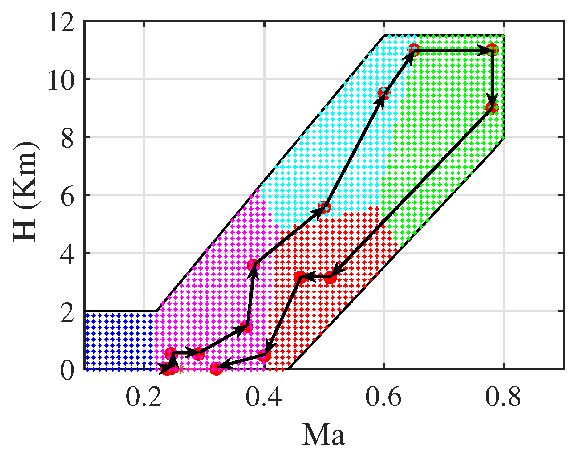
Figure 1. Uncertain switched system structure.
Energies 14 05204 g001
Figure 2. The control structure for the uncertain switched system.
Energies 14 05204 g002
Figure 3. Discontinuous Lyapunov functions (for l = 3).
Energies 14 05204 g003
Figure 4. Case 1 proof.
Energies 14 05204 g004
Figure 5. The operating envelope and flight profile.
Energies 14 05204 g005
Figure 6. Switching signal.
Energies 14 05204 g006
Figure 7. Fan speed N 1 .
Energies 14 05204 g007
Figure 8. Fuel flow.
Energies 14 05204 g008
Figure 9. Switching signal with the resetting scheme.
Energies 14 05204 g009
Figure 10. Switching signal without the resetting scheme.
Energies 14 05204 g010
Figure 11. Fan speed N 1 .
Energies 14 05204 g011
Figure 12. Fuel flow.
Energies 14 05204 g012
Figure 13. Sub-controller switching signals.
Energies 14 05204 g013
Figure 14. Fan speed N 1 tracking.
Energies 14 05204 g014
Figure 15. Tracking error of fan speed N 1 .
Energies 14 05204 g015
Figure 16. High-pressure rotor speed N 2 .
Energies 14 05204 g016
Figure 17. Fuel flow.
Energies 14 05204 g017
Figure 18. Thrust.
Figure 18. Thrust.
Energies 14 05204 g018
Table 1. Nominal points for seven subregions.
No. Ma H (m) N 1 (rpm)
1001800
2003200
30.3110001700
40.3110003200
50.640003200
60.7880003200
70.7810,0003200
Publisher’s Note: MDPI stays neutral with regard to jurisdictional claims in published maps and institutional affiliations.

