A Machine Learning-Based Gradient Boosting Regression Approach for Wind Power Production Forecasting: A Step towards Smart Grid Environments

Abstract

In the last few years, several countries have accomplished their determined renewable energy targets to achieve their future energy requirements with the foremost aim to encourage sustainable growth with reduced emissions, mainly through the implementation of wind and solar energy. In the present study, we propose and compare five optimized robust regression machine learning methods, namely, random forest, gradient boosting machine (GBM), k-nearest neighbor (kNN), decision-tree, and extra tree regression, which are applied to improve the forecasting accuracy of short-term wind energy generation in the Turkish wind farms, situated in the west of Turkey, on the basis of a historic data of the wind speed and direction. Polar diagrams are plotted and the impacts of input variables such as the wind speed and direction on the wind energy generation are examined. Scatter curves depicting relationships between the wind speed and the produced turbine power are plotted for all of the methods and the predicted average wind power is compared with the real average power from the turbine with the help of the plotted error curves. The results demonstrate the superior forecasting performance of the algorithm incorporating gradient boosting machine regression.

1. Introduction

In recent years, renewable energy sources (RES) have become a center of exploration due to the advantages they are providing to power systems. As the penetration of RES intensifies, the associated challenges in power systems are also escalated. Among various renewable energy resources, wind energy has gathered ample importance due to its sustainability, non-polluting, and free nature [1,2]. Irrespective of the various advantages of wind power, errorless power prediction for wind energy is a very difficult task. Both the climatic and various seasonal effects are not only the factors influencing the generation of wind power, but the intermittent nature of wind itself also makes it increasingly complicated to forecast [3]. Wind energy is critically important for the social and economic growth of any country. Considering this, reliable and precise wind power prediction is crucial for the dispatch, unit commitment, and stable functioning of power systems. This makes it easier for grid operators of the power system to support uniform power distribution, reduce energy loses, and optimize power output [4,5]. Besides this, without the functionality of forecasting, wind energy systems that are extremely disorganized can cause irregularities and brings about great challenges to a power system. Consequently, the integration of wind power globally relies on correct wind power prediction. It is necessary to develop dedicated software in this regard, where weather forecast data and wind speed data are model inputs and would predict the power that a wind farm or a particular wind turbine could produce on a particular day. Furthermore, forecasted outputs could be analyzed in terms of a town’s actual per-day power demands [6,7,8]. When the forecasted power is not sufficient to meet the daily requirements of the town, then adequate decisions could be taken to arrange leftover power to be gathered from other sources. In the case that the forecasted power exceeds the demand, then a suitable number of wind turbines could be turned off to prevent surplus generation [9]. This approach has the capability of reducing repeated power outages and protecting generated power from being wasted. Many researchers, e.g., Pathak et al. [10], Chaudhary et al. [11], and Zameer et al. [12], have been performing research to develop optimized software models for forecasting power generation via RES.

Many of these algorithms have not produced acceptable results for different wind farm locations in which forecasting has been carried out with erratic and turbulent wind conditions. Under these circumstances, the number of required input variables substantially increases [13]. Nowadays, ML-based regression forecasting techniques such as support vector regression models and auto-regression, among others, are very prominent [14,15]. These techniques are used in power generation and consumption, electric load forecasting, solar irradiance prediction for photovoltaic systems, grid management, and wind energy production. A reliable and accurate forecasting algorithm is essential for wind power production [16,17].

Noman et al. [18] investigated a support vector machine (SVM)-based regression algorithm for predicting wind power in Estonia one day in advance. Wu et al. [19] suggested a new spatiotemporal correlation model (STCM) for ultrashort-term wind power prediction based on convolutional neural networks and long short-term memory (CNN-LSTM). The STCM based on CNN-LSTM has been used for the collection of metrological factors at various places. The outcomes have shown that the proposed STCM based on CNN-LSTM has a superior spatial and temporal characteristic extraction ability than traditional models. Yang et al. [20] developed a fuzzy C-means (FCM) clustering algorithm for the forecasting of wind energy one day in advance to reduce wind energy output differences. Li et al. [21] proposed the combination of a support vector machine (SVM) with an enhanced dragonfly algorithm to predict short-term wind energy. The improved dragonfly algorithm selected the optimal parameters of SVM. The dataset was collected from the La Haute Borne wind farm in France. The developed model showed improved forecasting performance as compared with Gaussian process and back propagation neural networks. Lin et al. [22] constructed a deep learning neural network to forecast wind power based on SCADA data with a sampling rate of 1 s. Initially, eleven input parameters were used, including four wind speeds at varying heights, the ambient temperature, yaw error, nacelle orientation, average blade pitch angle, and three measured pitch angles of each blade. A comparison between various input parameters showed that the ambient temperature, yaw error, and nacelle positioning could be areas for optimization in deep learning models. The simulation outcome showed that the suggested technique could minimize the time and computational costs and provide high accuracy for wind energy prediction.

Wang et al. [23] proposed an approach for wind power forecasting using a hybrid Laguerre neural network and singular spectrum analysis. Wang et al. [24] presented a deep belief network (DBN) with a k-means clustering algorithm to better deal with wind and numerical prediction datasets to predict wind power generation. A numerical weather prediction dataset was utilized as an input for the proposed model. Dolara et al. [25] used a feedforward artificial neural network for the accurate forecasting of wind power. Their results were compared with predictions provided by numerical weather prediction (NWP) models. Abhinav et al. [26] presented a wavelet-based neural network (WNN) for forecasting the wind power for all seasons of the year. The results showed better accuracy for the model with less historic data. Yu et al. [27] suggested long- and short-term memory-enriched forget gate network models for wind energy forecasting. Zheng et al. [28] suggested a double-stage hierarchical ANFIS to forecast short-term wind energy.

To predict the wind speed and turbine hub height, the ANFIS first stage employs NWP, while the second stage employs actual power and wind speed relationships. Jiang et al. [29] developed an approach to enhance the power prediction capabilities of a traditional ARMA model using a multi-step forecasting approach and a boosting algorithm. Zhang et al. [30] evolved an autoregressive dynamic adaptive (ARDA) model by improving the autoregressive (AR) model. In this approach, a fixed parameter estimation method for the autoregressive model was enhanced to a dynamically adaptive stepwise parameter estimation method. Later on, the results were compared with those of the ARIMA and LSTM models. Qin et al. [31] developed a hybrid optimization technique which combined a firefly algorithm, long short-term memory (LSTM) neural network, minimum redundancy algorithm (MRA), and variational mode decomposition (VMD) to improve wind power forecasting accuracy. Huang et al. [32] used an artificial recurrent neural network for forecasting. Recently, some researchers have developed their own optimization approaches, such as in [33,34], where the authors developed sequence transfer correction and rolling long short-term memory (R-LSTM) algorithms. Akhtar et al. [35] constructed a fuzzy logic model by taking the air density and wind speed as input parameters for the fuzzy system used for wind power forecasting.

Aly et al. [36] developed a model to forecast wind power and speed using various combinations, including a wavelet neural network (WNN), artificial neural network (ANN), Fourier series (FS) and recurrent Kalman filter (RKF). Bo et al. [37] proposed nonparametric kernel density estimation (NPKDE), least square support vector machine (LSSVM), and whale optimization approaches for predicting short-term wind power. Li el al. [38] developed an ensemble approach consisting of partial least squares regression (PLSR), wavelet transformation, neural networks, and feature selection generation for forecasting at a wind farm. Colak et al. [39] proposed the use of moving average (MA), autoregressive integrated moving average (ARIMA), weighted moving average (WMA), and autoregressive moving average (ARMA) models for the estimation of wind energy generation. Saman et al. [40] proposed six distinct machine heuristic AI-based algorithms to forecast wind speeds by utilizing meteorological variables. Yan et al. [41] investigated a two-step hybrid model which used both data mining and a physical approach to predict wind energy three months in advance for a wind farm. From the literature survey, it is clear that there have been several research studies that have investigated the forecasting of wind energy by employing various analytical approaches across several horizons, among which persistence and statistical approaches have been used. Statistical approaches have not been suitable approaches for forecasting wind power as they have not been able to handle huge datasets, adapt to nonlinear wind dataset, or make long-term predictions [42,43,44].

Prior to our research, there have been many types of prediction models that have been shaped to predict wind energy, namely, physical models, statistical models, and teaching and learning-based models, which employ machine learning (ML) and artificial intelligence (AI)-based algorithms. Current studies typically adopt machine learning algorithms (ML). In particular, naive Bayes, SVM, logistic regression, and deep learning architectures of long short-term memory networks are typically used.

In the present study, the primary reason for adopting ML algorithms is that they can adapt themselves to changes with regards to the location of wind farms. Varying locations can have more erratic and turbulent trends, and thus generating predictive models on the basis of an input dataset instead of utilizing a generalized model is of importance. The foremost contribution of this research is short-term wind power forecasting on the basis of the historical values of wind speed, wind direction, and wind power by using ML algorithms. Furthermore, short-term wind power forecasts are analyzed compared to the forecasting of long-term wind power, as the algorithms and methods are unable to deliver satisfying results at high precision with respect to wind speed forecasting in this regard. In this study, regression algorithms such as random forest, k-nearest neighbor (k-NN), gradient boosting machine (GBM), decision tree, and extra tree regression are employed to enhance the forecasting accuracy for wind power production for a Turkish wind farm situated in the west of Turkey. Regression algorithms have been applied because of forecasting problems encountered with continuous wind power values. Polar curves have been plotted and the impacts of input variables such as the wind speed and direction on wind energy generation is examined. Scatter curves depicting the relationships between the wind speed and the produced turbine power are plotted for all of the methods here and the predicted average wind power is compared with the real average power from a turbine with the help of the plotted error curves. The results demonstrate the superior forecasting performance of gradient boosting machine regression algorithm considered here.

The paper is organized in six sections. Section 2 describes the proposed model, followed by the preprocessing of the SCADA data in Section 3. Section 4 presents the machine learning techniques used to enhance the forecasting accuracy. Section 5 deliberates upon the results and presents a discussion. Finally, the conclusions of this work are outlined in Section 6.

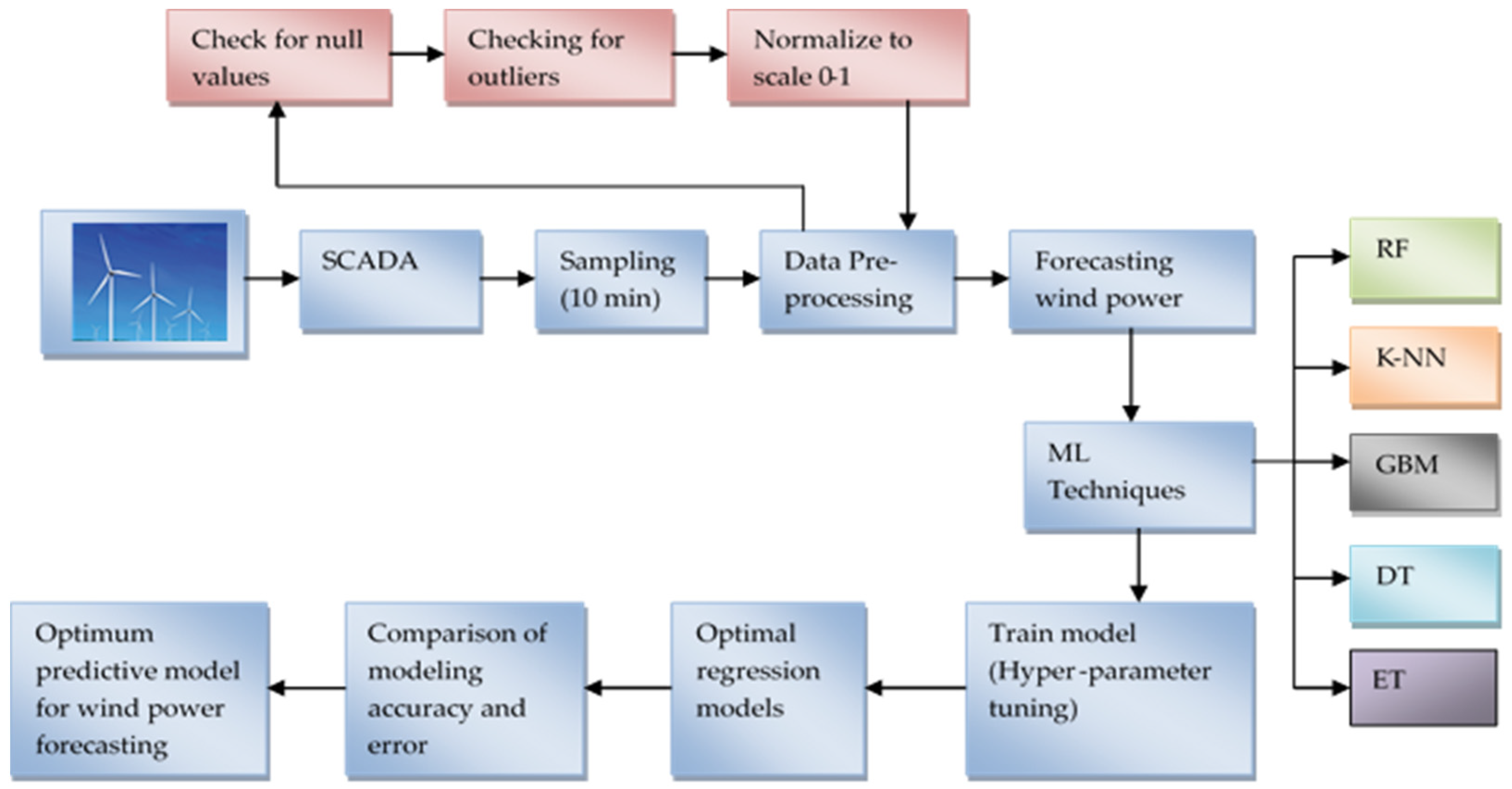
2. Proposed Model

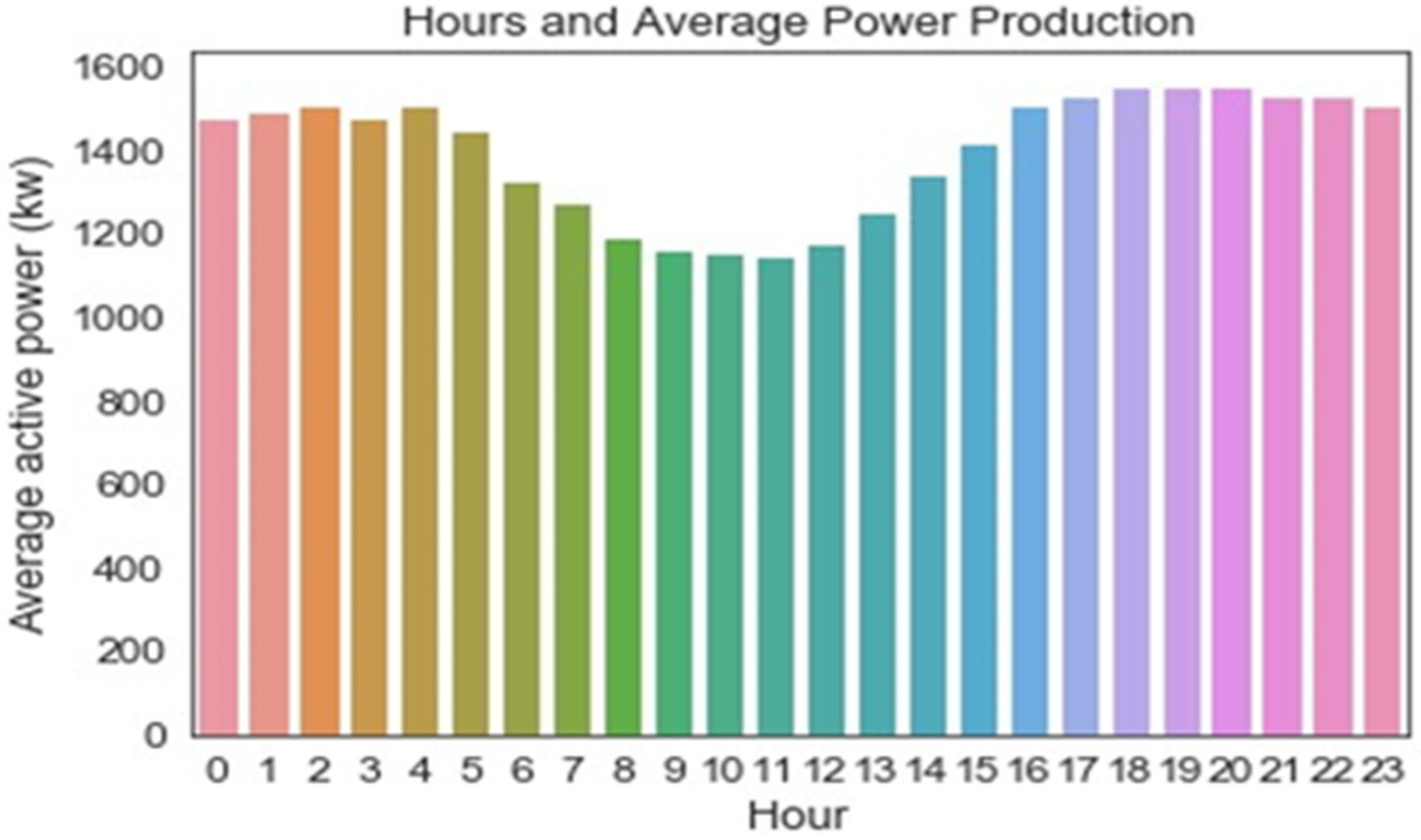
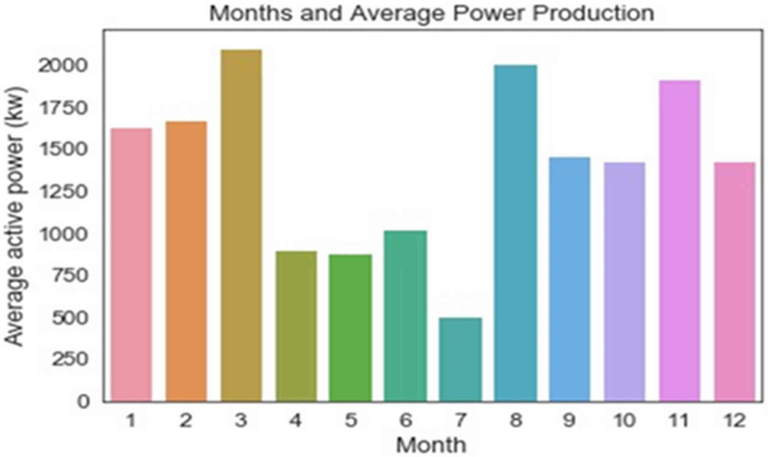
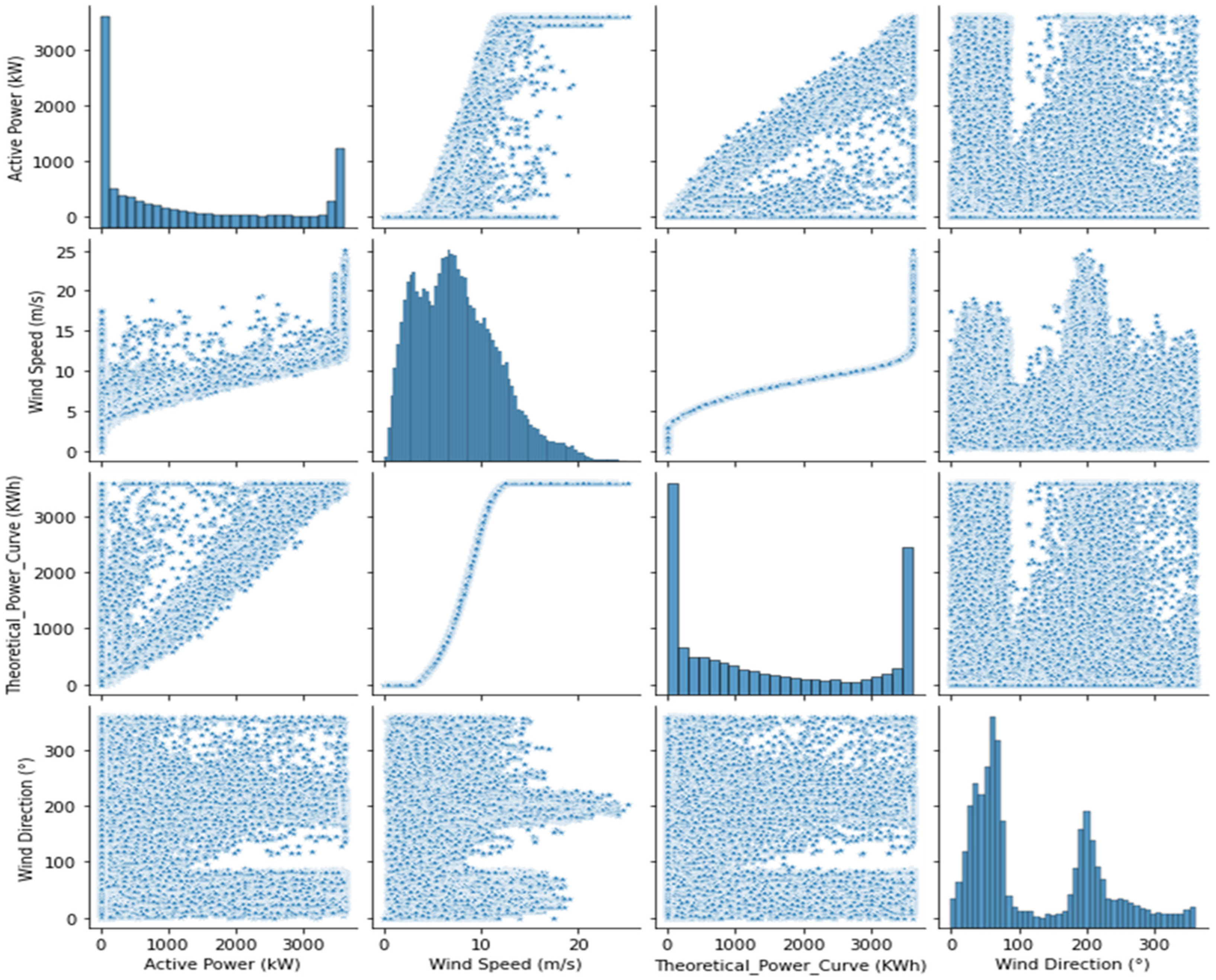
2.1. Input Metrological Parameters

This section is devoted to estimate suitable input parameters that will affect the active power of wind turbine, considering the wind farm layout. The selected variables are the exogenous inputs of the machine learning algorithms. The data analysis for forecasting has been accomplished via a freely accessible dataset containing data for a northwestern region of Turkey [45]. The wind farm considered in this study is the onshore Yalova wind farm, featuring 36 wind turbines with total generation capacity of 54,000 kW according to www.tureb.com.tr/bilgi-bankasi/turkiye-res-durumu (accessed on 18 May 2020). The facility has been in operation since 2016.

2.2. Predictive Analysis

The steps involved in predictive analysis are illustrated in Figure 1. Data exploration is the initial step in the analysis of data and is where users explore a large dataset in an unstructured way to discover initial patterns, points of attention, and notable characteristics. Data cleaning refers to identifying the irrelevant, inaccurate, incomplete, incorrect, or missing parts of the data and then amending, replacing, and removing data in accordance with the requirements. Modeling denotes training the machine learning algorithm to forecast the levels from the structures and then tuning and validating for the holdout data. The performance of machine learning algorithm is evaluated by different performance metrics using training and testing datasets.

The proposed model for the data analysis and forecasting is illustrated in Figure 2. A supervisory control and data acquisition (SCADA) system has been employed to measure and save wind turbines dataset. The SCADA system captures the wind speed, wind direction, produced power, and theoretical power based on the turbine’s power curve. Every new line of the dataset is captured at a 10 min time interval and the time period of the dataset is one year. The data are accessible in the CSV format.

Table 1. Information for the wind turbine (Yalova wind farm, Turkey).

Input Variables	Wind Speed, Wind Direction, Theoretical Power, Active Power
Draft Frequency	10 min
Start Period	1 January 2018
End Period	31 December 2018

presents the dataset information for the wind turbine. The wind turbine technical specifications are given in

Table 2. Wind turbine technical specifications.

Characteristics	Wind Turbine
SINOVEL (turbine manufacturer)	SL1500/90 (Turbine model)
Rated Power	1.5 MW
Hub Height	100 m
Rotor Diameter	90 m
Swept Area	6362 m2
Blades	3
Cut-in Speed of Wind	3 m/s
Rated Speed of Wind	10 m/s
Cut-off Speed of Wind	22 m/s

, although there are a quite few gaps and at some points generated output power is absent, which may be due to wind turbine maintenance, malfunction, or lower wind speed than the operation speed. The dataset contains a total of 50,530 observations, and 3497 data points were considered as outliers because of zero power production. After removing outliers or missing values, the rest of the dataset, i.e., 47,033 data points, were considered for implementing the machine learning models. The dataset consisted of two parts, namely, the training set, containing the first 70% of the whole dataset, and the testing set, containing the latter 30% of the dataset.

As stated in [46,47], the power curves of a wind turbine, when plotted between the cut-in speed, rated speed, and cut-out speed, can be established by an n degree algebraic equation (Equation (1)) for forecasting the power output of a wind turbine.

$$P_i(v)=\{\begin{array}{l}0,\hspace{1em}\hspace{1em}\hspace{1em}\hspace{1em}\hspace{1em}\hspace{1em}\hspace{1em}\hspace{1em}\hspace{1em}\hspace{1em}\hspace{1em}\hspace{1em}\hspace{1em}\hspace{1em}\hspace{1em}\hspace{1em} v<v_{ci}\\ \left(a_n{v}^n+a_{n-1}{v}^{n-1}+\dots +a_{1}v+a_0\right), v_{ci}\le v<v_{R }\\ P_R\hspace{1em}\hspace{1em}\hspace{1em}\hspace{1em}\hspace{1em}\hspace{1em}\hspace{1em}\hspace{1em}\hspace{1em}\hspace{1em}\hspace{1em}\hspace{1em}\hspace{1em}\hspace{1em} v_{ci}\le v<v_R\\ 0,\hspace{1em}\hspace{1em}\hspace{1em}\hspace{1em}\hspace{1em}\hspace{1em}\hspace{1em}\hspace{1em}\hspace{1em}\hspace{1em}\hspace{1em}\hspace{1em}\hspace{1em}\hspace{1em}\hspace{1em}\hspace{1em} v\ge v_{co}\end{array}$$

(1)

where $P_i\left(v\right)$ is power produced from the relative wind speed and the regression constants are given by $a_n a_{n-1 }{a}_1$ and $a_0$, $v_{ci}$ is the cut-in speed, $v_R$ is the rated speed, and $v_{co}$ is the cut-out speed. The energy output for a considered duration can be calculated by Equation (2):

$$E_c={\sum }_{i=1}^{N}P\left(v_i\right)∆t$$

(2)

where N denotes the number of hours in the study period and $∆t$ is the time interval [48]. The energy produced with a given wind speed can be appraised by multiplying the power produced by the wind turbine by wind speed $v$ and the time period for which the wind speed $v$ prevails at the given site. The overall energy generated by the turbine over a given period can be assessed by summing the energies corresponding to all possible wind speeds with the related conditions at points where the system is functional.

Figure 3 shows a plot of wind speed power scatter curves where the theoretical power generation curve usually fits with the real power generation. It may also be observed that the power generation curve reaches the maximum level and continues in a straight line when the wind speed reaches ~13 m/s. At wind speeds higher than 3 m/s (cut-in speed), there are some points of zero power generation, and this could be due to maintenance, sensor malfunction, degradation, and system processing errors.

Closer examination of the wind turbine power highlighted three anomaly types in the SCADA data of the wind turbine. Type-1 anomalies are displayed in the scatterplot via a horizontal dense cluster of data where the generation of power is zero at a wind speed higher than the cut-in speed. Such anomalies generally occur due to the turbine downtime that can be cross-referenced when utilizing an operation log [49,50]. Type-2 anomalies are shown by a dense cluster of data that fall below the ideal power curve of the wind turbine. These anomalies can occur because of wind curtailment, where the turbine output power is controlled by its operator to be lower than its operational capacity. Wind restriction can be executed by operators of a wind farm due to various reasons, such as difficulty in the storage of huge capacities of wind power, a lack of demand for power at several times, and at times where volatile wind conditions cause the produced electricity to be unstable in nature. Type-3 anomalies are arbitrarily dispersed around the curve and these are generally the result of sensor degradation or malfunction, or they may be due to noise at the time of signal processing [51,52]. It is also worth noting that a segment of type-2 and type-3 anomalies can also be illustrated by the dispersion produced on account of incoherent wind speed measurements taken as a result of turbulence.

Figure 4 shows hourly average power production over a day, while the monthly average power production is shown in Figure 5.

Figure 6 shows paired scatter plots describing the relationship of each feature with each other feature. The plots with a diagonal shape represent histograms showing the probability distribution of each weather feature. The lower and upper triangles display the scatter plots representing the relationships between the features. It is also seen that each feature demonstrates the distribution with other features. The paired scatter plots show the changes for one feature in comparison to all other features.

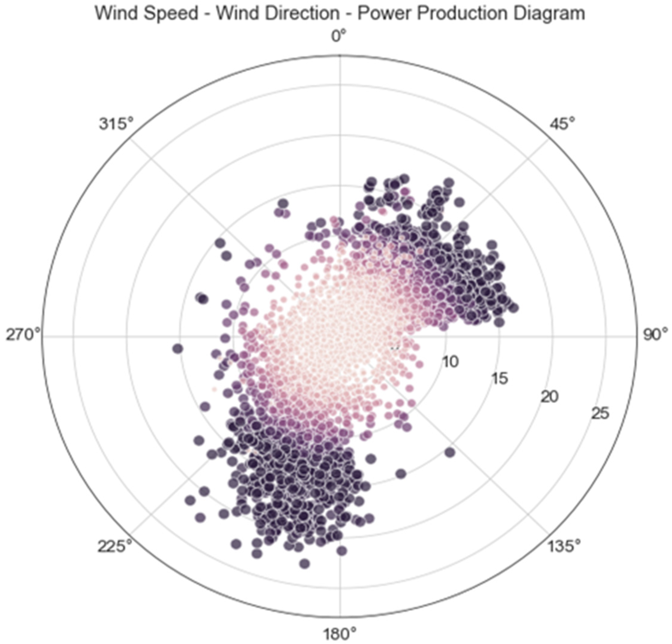
2.3. Analysis in Polar Coordinates

Figure 7 presents a polar diagram exhibiting the qualitative distribution of power generation with wind speed and wind direction from the sample dataset. It is clear from the polar diagram that the wind speed, wind direction, and power generation are vastly correlated, as wind turbine generates maximum power if the wind blows from a direction between 0–90 or 180–225 degrees. It is also seen from the polar diagram that there is no power generation beyond the cut-out speed of 22 m/s. Also, from some directions, very low power generation is taking place. The wind direction parameter is denoted by the radius of the polar graph. In the polar graph, light color points represent low power generation when the wind speed is below the cut-in speed (i.e., 3 m/s) of the wind turbine. As the speed of wind increases beyond the cut-in speed, power production increases, as represented by the dark and densely spaced points in the polar diagram.

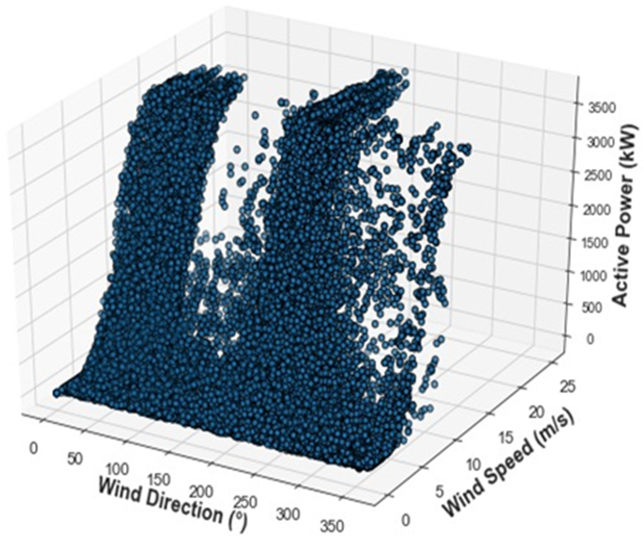
2.4. Analysis in Cartesian Coordinates

Figure 8 shows a three-dimensional quantitative visualization of the power generation with the wind speed and wind direction in a Cartesian coordinate system for the whole year. In Figure 8, it can be seen that the two regions that are dense contribute to the maximum power generation. The first region is observed when the direction of the wind varies from 0° to 90° and the second region is observed when the wind direction varies from 180° to 230°.

3. SCADA Pre-Processing

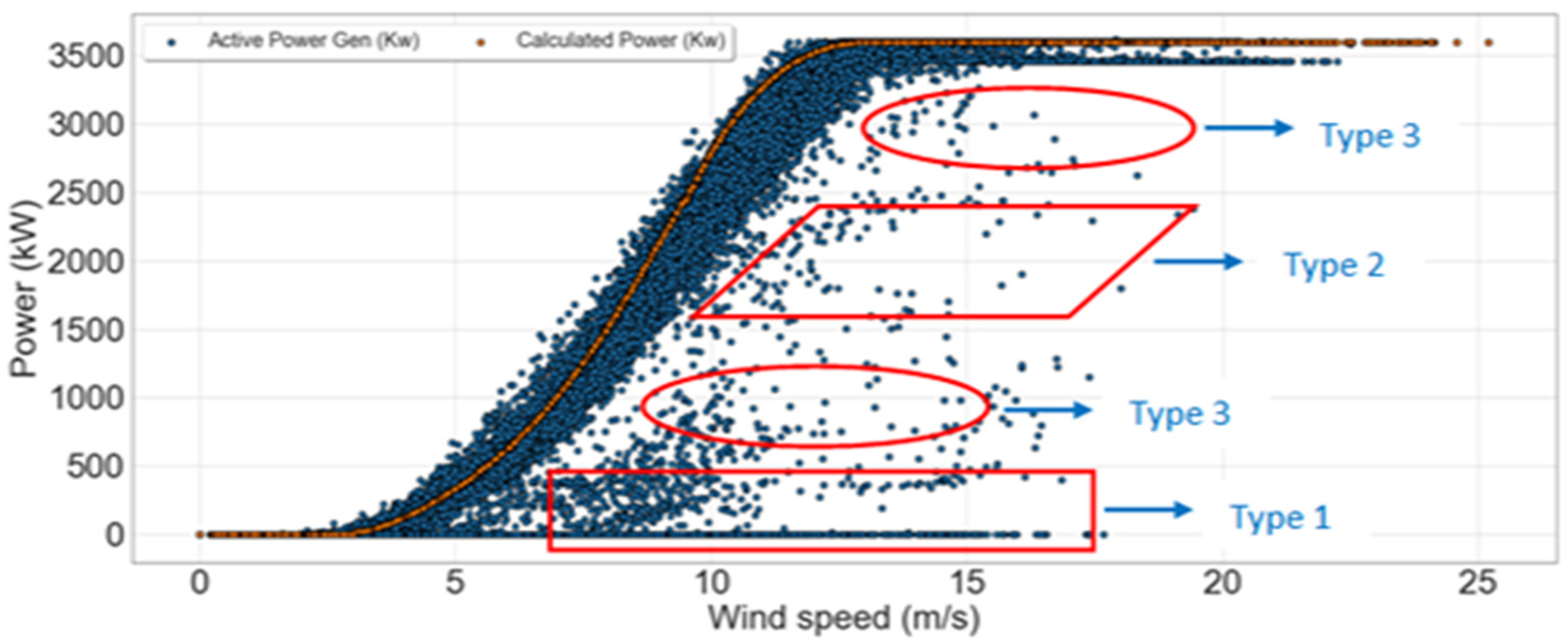
• Outlier removal: The procedure of cleaning and preparing the raw data to make it compatible for training or developing machine learning models is called data preprocessing. To limit the impact of noise and turbulence, a sampling rate of 10 min was used when processing the SCADA data; however, deep analysis of individual parameters identified certain errors in the SCADA data, such as, power production being zero above the cut-in speed (i.e., 3 m/s), negative values of wind speed, or active power and missing data at some timestamps. These results carry no practical significance in terms of the generation of power. As such, to prevent a negative impact on the forecasting, data points belonging to the same timestamp have been removed. Such erroneous data points are commonly the result of wind farm maintenance, sensor malfunction, degradation, or system processing errors. It is crucial that the SCADA data are pre-processed prior to developing the forecasting models.
• Normalization of dataset: The input parameters of the wind power forecasting model incorporate the wind speed and wind direction, but their dimensions are not of the same order of magnitude. Hence, it is essential to regulate these input vectors to be within in the same order of magnitude. As such, a min-max approach was used to normalize the input vectors as follows:

  $$\overline{x}=\frac{x-x_{min}}{x_{max}-x_{min}}$$

  (3)

  where the actual data is given by $x$ and $x_{min}$ and $x_{max}$ represent the minimum and maximum values of the dataset. The result $\overline{x}$ remains within the range of [0,1].

4. Machine Learning

Machine learning is a solicitation of AI (artificial intelligence) that offers automatically learning capabilities for systems and the ability to learn from experiences without being explicitly programmed to do so. Machine learning algorithms exhibit a dataset-based behavior and model input features corresponding to the desired output, thereby forecasting output features by learning from a historic dataset. ML is essential for prediction here due to the following reasons: Firstly, ML gives best performance when the input and output relationship is not clear. It also improves in terms of decision making or predictive accuracy over time. ML algorithms can easily identify changes in the environment and adapt themselves according to the new environment; however, there are several machine algorithms, each of which is specifically utilized for applications or problems. For instance, regression and classification algorithms are mainly used for forecasting problems. ML also has the ability to handle complex systems. We implemented five regression analysis algorithms, namely random forest regression, k-nearest neighbor regression (k-NN), gradient boosting machine regression (GBM), decision tree regression, and extra tree regression. These algorithms were selected based on good performance and extensive usage in the literature. These algorithms have distinct theoretical backgrounds in forecasting problems, where they have provided results successfully. Additionally, these algorithms have various parameters known as hyper-parameters which affect the runtime, generalization capability, robustness, and predictive performance. We have adopted a trial-and-error approach to select the best parameters for algorithms, and this is known as hyper-parameter tuning. Also, for the best observed outputs, the values of these parameters for each regression algorithm are placed at the bottom of the section for each algorithm.

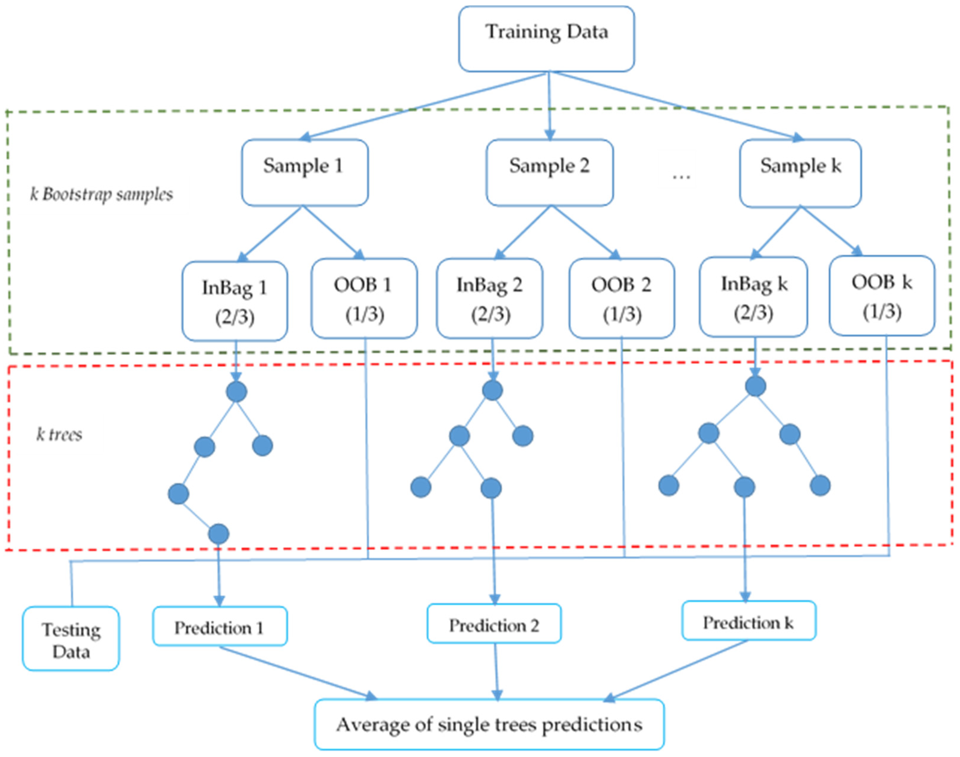
4.1. Random Forest Regression

Random forest (RF) regression is a famous decision tree algorithm where multiple decision trees are produced from a given input dataset. First, the algorithm divides the dataset randomly into several sub-parts and for each subpart it builds multiple decision trees. Then, it merges the predicted output of each decision tree to obtain a more stable and accurate prediction. In RF regression, the output value of any input or subset is a mean of the values predicted by several decision trees. The following process is performed:

• Produce n_tree bootstrap samples from the actual input dataset;
• For individual bootstrap samples, expand an unpruned regression tree, including subsequent alteration at every node, instead of selecting the best split among all predictors. Arbitrarily sample m_try predictors and then select the best split from those variables. (“Bagging” can be considered a special case of RF and where m_try = p predictors. Bagging refers to bootstrap aggregating, i.e., building multiple distinct decision trees from training dataset by frequently utilizing multiple bootstrapped subsets of the dataset after averaging the models);
• Estimate new data values by averaging the predictions of the n_tree, decision trees (i.e., “average” in case of problems of regression and the “majority of votes” for classification problems);
• Based on the training data, the error rate can be anticipated using the following steps:
  • At each bootstrap iteration, predict data not in the bootstrap sample (as Breiman calls “out of bag” data) by utilizing the tree developed with the bootstrap sample.
  • Averaging the out of bag predictions, on the aggregate, where each data value would be out of bag around 36% of the times and hence averaging those predictions.
  • Compute the error rate and name it the “out of bag” estimate of the error rate.

In practice, we have observed that out of bag estimation of the error rate is fairly truthful, provided that large numbers of trees are grown, otherwise the bias condition may occur in the “out of bag” estimate. A complete flowchart for the process can be seen in Figure 9. In this model, the random state was chosen as 40 and the number of trees was selected as 100, as increasing the number of tress to larger than 100 did not significantly improve the forecasting output. Also, an appropriate number of trees is required to be chosen to optimize the forecasting performance and runtime. Figure 10a shows a scatter plot depicting the relationship between the wind speed (m/s) and the power produced (kW) by the turbine when using random forest regression. Figure 10b presents the predicted average of wind power as compared with real average power from turbine (kW) when using random forest regression.

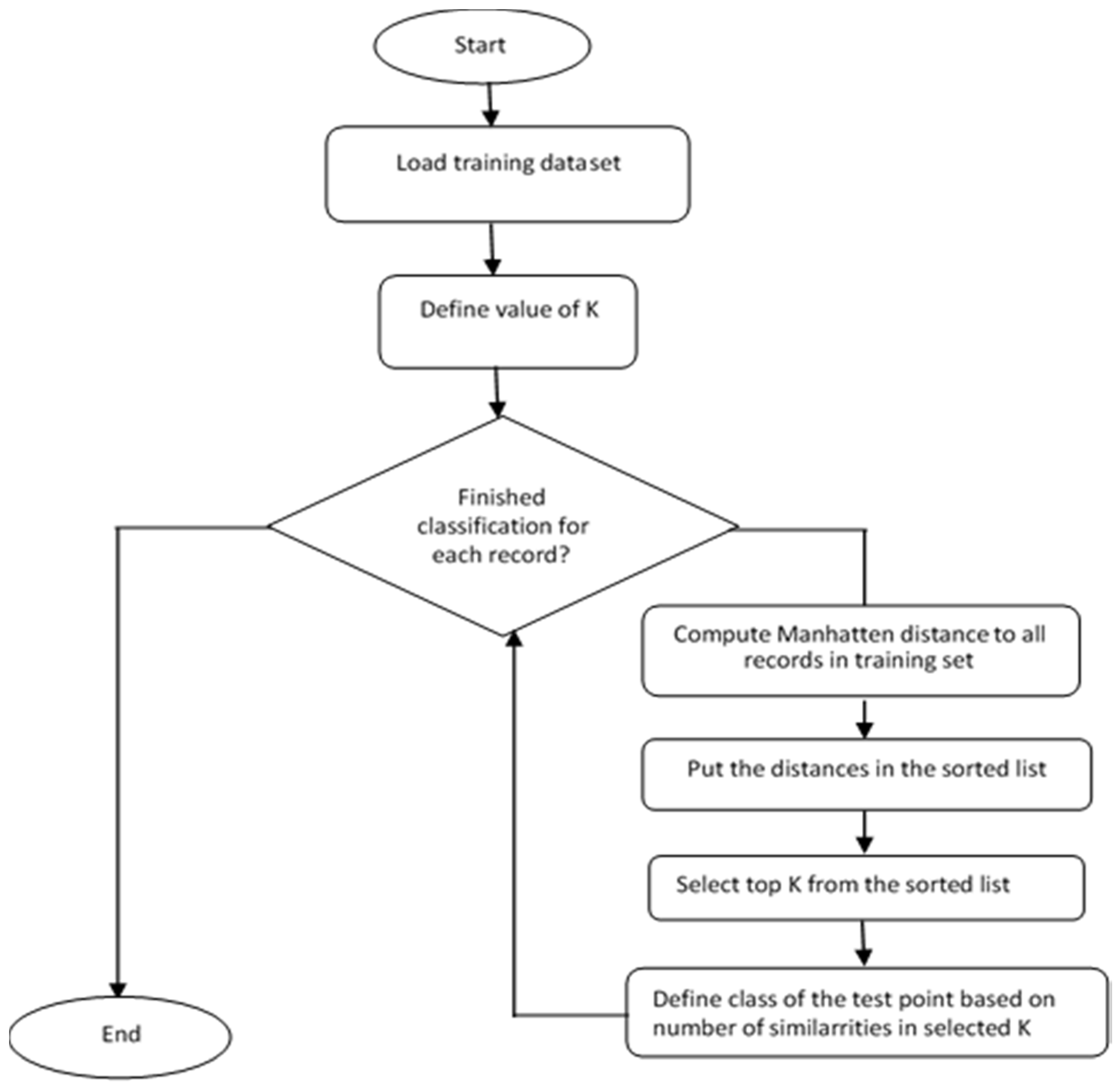
4.2. k-Nearest Neighbor Regression

k-Nearest Neighbor (k-NN) regression is one of the most simple, easy to implement, non-parametric regression approaches used in machine learning. The main objective behind k-nearest neighbor regression is that whenever a new data point is to be predicted, the point’s k nearest neighbors are nominated from the training-dataset. Accordingly, the prediction of a new data point will be the average of the values of the k-nearest neighbors. The basis of the k-nearest neighbor algorithm can be outlined in three major steps:

• Compute the predefined distance between the testing dataset and training dataset;
• Select k-nearest neighbors with k-minimum distances from the training dataset;
• Predict the final renewable energy output based on a weighted averaging approach.

A distance measure is needed to distinguish the similarity between two instances. The Manhattan and Euclidean distances are widely used distance metrics in this regard [53]. In the present study, the actual Manhattan distance was improved by the use of weighting. The weighted Manhattan distance is determined by the following:

$$D\left[X^i,X^j\right]={\displaystyle \sum }_{n=1}^r{w}_n\left|x_n^{\left(i\right)}-x_n^{\left(j\right)}\right|$$

(4)

where $X^i$ and $X^j$ are two instances and there are r attributions for each instance, i.e., $X=\left[x_1,\dots ,x_n,\dots ,x_r\right]$ and $w_n$ is the weight allocated to nth attribution. The weight $w_n$ equals 1 in the original Manhattan distance and denotes an equal contribution of each attribute to distance D. The significance of each attribution is quite distinct in renewable power generation forecasts. The $w_n$ weight considers the contribution of every variable to the distance and would be computed by the process of optimization. Prediction is performed based on the linked target values once the value of k-nearest neighbors is determined. Consider that $X^1,\dots ,X^K$ indicates the k-nearest instances that are nearest to testing instance $X$, and their power outputs are shown by $p^1,\dots ,p^K$. The distance between the k-nearest neighbor and $X$ follows the ascending order of $d^1\le \dots \le d^K$ where $d^K$ = D[$X,X^k]$(k = 1,...,$K).$ In terms of renewable power production, point prediction is estimated with an average weighed through exponential function as follows:

$$\overbrace{p}=\sum _{k=1}^K{\delta }^k{p}^k=\frac{{\sum }_{k=1}^K{e}^{-d^k}.p^k}{{\sum }_{k=1}^K{e}^{-d^k}}$$

(5)

where $d^k$ and $p^k$ are distances associated with the instance $X^k$ and the renewable power output, correspondingly. Figure 11 presents a flowchart of the k-nearest neighbor regression method. In this paper, k was selected as 7 and the Manhattan distance was chosen as the distance measure.

Figure 12a shows a scatter plot depicting the relationship between the wind speed (m/s) and the power produced (kW) and Figure 12b presents the error curves, showing the comparison of forecasted average power with the real average power (kW) when using k-nearest neighbor regression.

4.3. Gradient Boosting Trees

Gradient boosting regression tree algorithms involve an ensemble learning approach where robust forecasting models are formed by integrating several individual regression trees (decision trees) that are referred to as weak learners. Such an algorithm reduces the error rate of weakly learned models (regressors or classifiers). Weakly learned models are those which have a high bias regarding the training dataset, with low variance and regularization, and whose outputs are considered only somewhat improved when compared with arbitrary guesses. Generally, boosting algorithms contains three components, namely, an additive model, weak learners, and a loss function. The algorithm can represent non-linear relationships like wind power curves and uses a range of differentiable loss functions and can inherently learn during iterations between input features [54]. GBM (gradient boosting machines) operate by identifying the limitations of weak models via gradients. This is attained with the help of an iterative approach, where the task is to finally join base learners to decrease forecast errors, where decision trees are combined by means of an additive model while reducing the loss function via gradient descent. The GBT (gradient boosting tree) $F_n\left(x_t\right)$ can be defined as the summation of $n$ regression-trees.

$$F_n\left(x_t\right)={\sum }_{i=1}^n{f}_i\left(x_t\right)$$

(6)

where every $f_i\left(x_t\right)$ is a decision tree (regression-tree). The ensemble of trees is constructed sequentially by estimating the new decision tree $f_{n+1}\left(x_t\right)$ with the help of the following equation:

$$argmin{\displaystyle \sum }_{t}L\left(y_t.F_n\left(x_t\right)+f_{n+1}\left(x_t\right)\right)$$

(7)

where L(·) is differentiable for loss-function L(·). This optimization is solved by a steepest descent method. In this study, a learning rate of 0.2 and estimator value of 100 were selected. A smaller learning rate makes it easier to stop prior to over fitting. Figure 13a presents a scatter plot depicting the relationship between the wind speed (m/s) and the power production (kW) of the turbine, and Figure 13b presents the error curves of the predicted average power in comparison with the real average power of the turbine (kW) when using gradient boosting regression.

4.4. Decision Regression Trees

A decision tree algorithm is an efficacious algorithm in machine learning which is utilized in supervised learning. This algorithm can be used to solve both regression and classification tasks. In decision analysis, it can be employed to explicitly and visually show both decisions and decision making. The foremost objective of using the algorithm is to produce a training model which can be used to forecast the value of the target variable with the help of learning modest judgment principles inferred from the training data [55]. As the name goes, it has a simple tree-like structure of decisions. In a decision tree, each node depicts a conditional statement and the branches of it show the outcome of the statement shown by the nodes. The algorithm iterates from the root node (highest node) to leaf nodes (bottom-most nodes). After executing all attributes in the nodes above, the leaf node (terminal node) shows the decision formed. This approach is considerably more accurate than SVM and ANN techniques.

The input to the algorithm includes training record $E$ and attribute set $F$. The algorithm functions by recursively selecting the best feature in order to split the data and increases the leaf nodes of the tree until the ending criterion is encountered (Algorithm 1).

Algorithm 1. Tree Growth ($E$, $F$).

1. if stopping _cond ($E$, $F$) = $true$ then

2.   leaf = createNode()

3.   $leaf.label$ Classify($E$)

4.   return $leaf$

5. else

6.   $root$ = create Node()

7.   $root.test\_cond$ = find_best_split($E$, $F$)

8.  let $V=\{ v|v$ is a possible outcome of $root.test\_cond\}$

9. for each $v\in V$ do

10.$E_v=\{e | root.test\_cond\left(e\right)=v and e\in E\}$

11.$child=$ TreeGrowth ($E_{v}F$)

12. add $child$ as descendent of $root$ and label the edge ($root\to child$) as $v$

13.   end for

14. end if

15. return root

In this study, the decision tree depth was selected as 17. In general, if the decision tree depth is greater, then the complexity of the model increases as the number of splits increases and contains more information about the dataset. This is the main reason for overfitting with DTs, where the model is perfectly fit with the training dataset and will not be able to generalize well with the testing dataset. In addition, a very low depth causes model under-fitting. Figure 14a presents a scatter plot depicting the relationship between the wind speed (m/s) and the power production (kW) of the turbine and Figure 14b shows the predicted average power in comparison with real average power of the turbine (kW) when using decision tree regression.

4.5. Extra Tree Regression

Extra tree or extremely randomized tree regression algorithms involve an ensemble machine learning technique. The algorithm has been evolved as an expansion of random forest algorithm, but the main difference is that it randomly chooses cut points partly or completely, with individual attributes, and selects splits. Extra tree regression utilizes the same rule as the RF algorithm and uses a random subset of topographies to train each base estimator. The nodes above the leaf node (the terminal node) show the decision that is formed. This approach is considerably more accurate than SVM and ANN techniques [51]. This algorithm randomly selects the paramount features, along with the consistent value for splitting a node; however, rather than selecting the most discriminative split in each mode [56,57,58], the extra tree approach utilizes the whole training dataset to train each regression tree. On the other hand, the RF algorithm utilizes a bootstrap replica to train the forecast model. These significant differences makes extra tree regression less likely to overfit a dataset, as there is better reported performance in the nodes above the leaf node (terminal node).

In the present study, the number of trees was selected as 90 and the maximum depth of trees was selected as 14. Generally, deeper tree sizes result in better performance. For extra tree regression, trees deeper than 14 started to depreciate the model performance. A maximum depth of six did not perform significantly better as the performance metrics were approximately equal. At a maximum depth of two, the model became under-fitted, resulting in lower R² values and higher values for performance matrices. Figure 15a presents a scatter plot depicting the relationship between the wind speed (m/s) and the power production (kW) of the turbine and Figure 15b shows the predicted average power in comparison with the real power of the turbine from turbine (kW) when using extra tree regression.

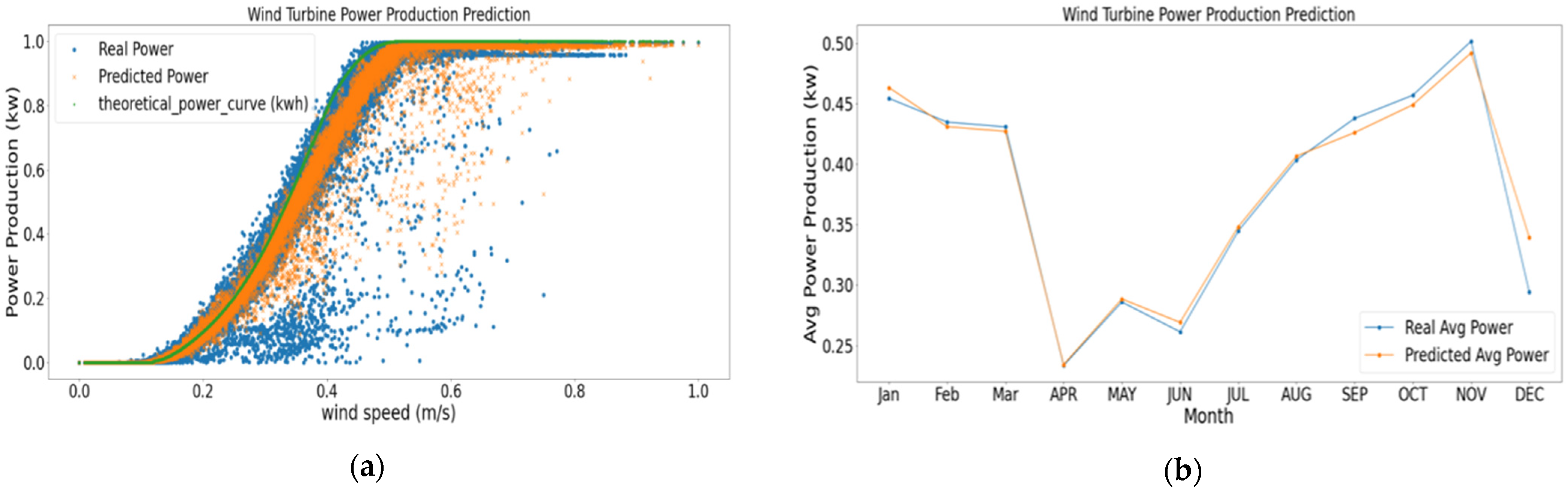
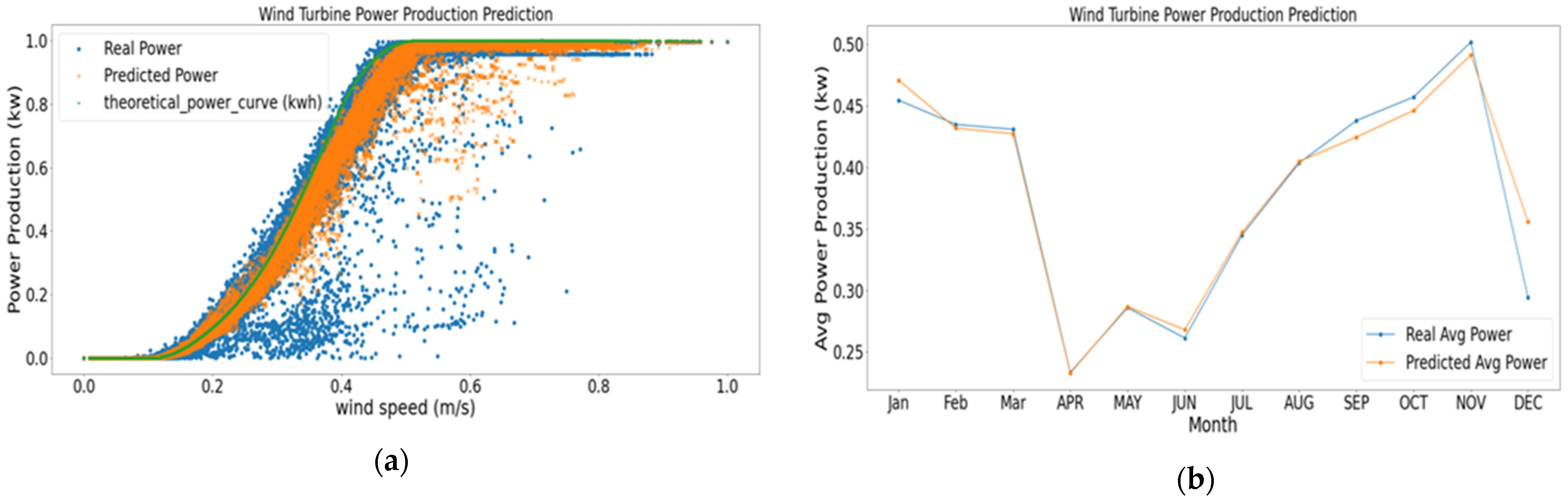
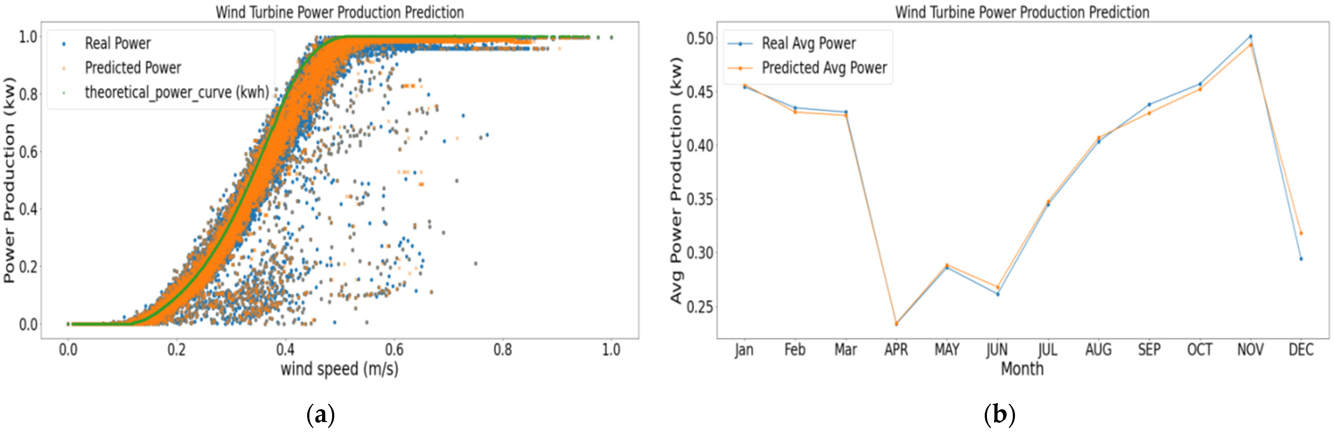
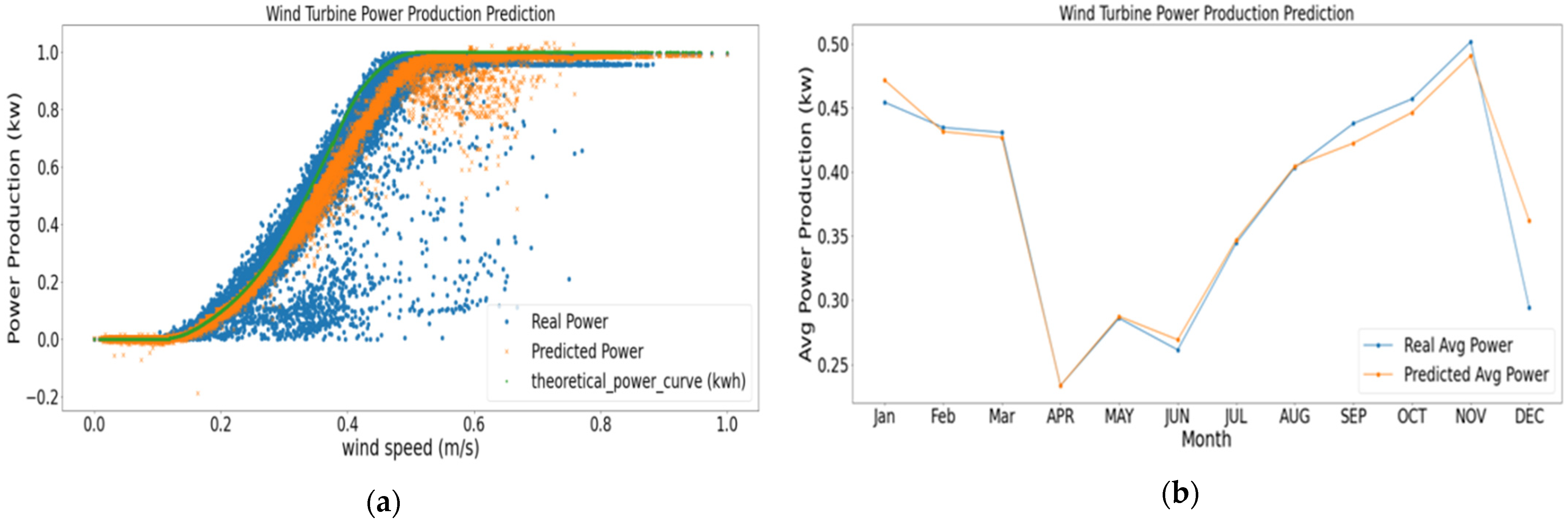
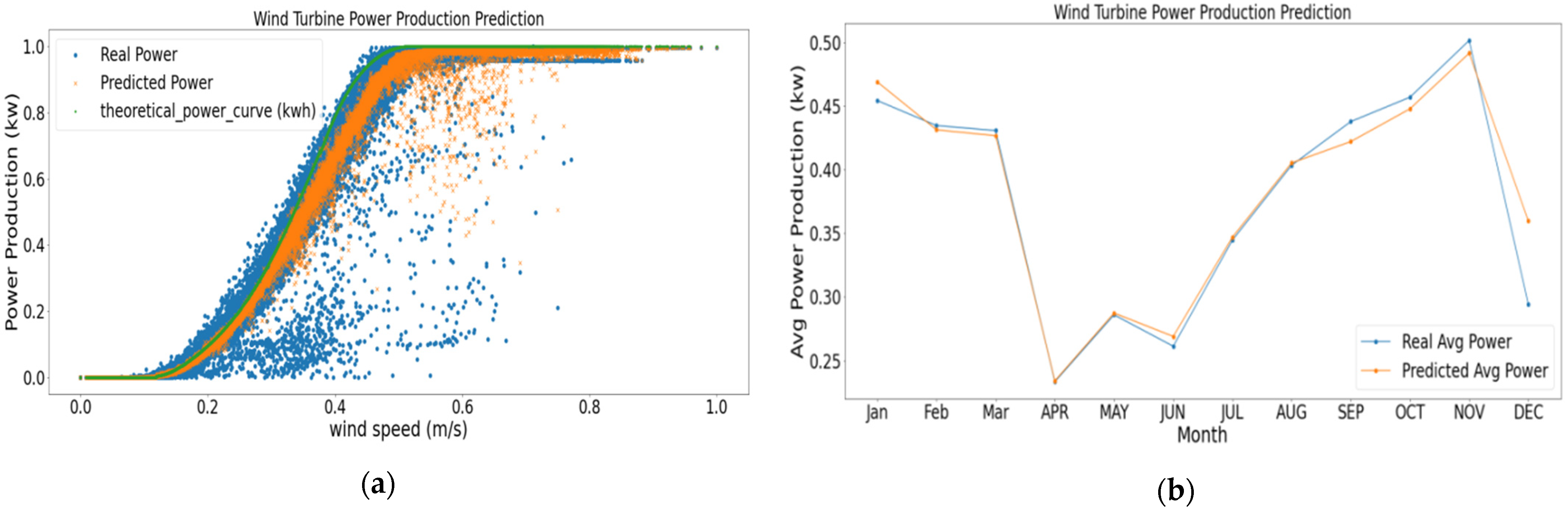
5. Results and Discussions

Based on the study performed in the above sections, the present section scrutinizes the outcomes and the key observations accomplished from the performances of the various regression models after programming for the forecasting of wind power. All models mentioned and explained above were trained and tested on a machine featuring 12 GB of 16 MHz DDR3 RAM and a 1.6 GHz Intel Core i5 processor running in a Jupiter notebook (Python 3.9.5 version) development environment.

Several hyper-parameters, such as the learning rate, size of trees (depth), and regularization parameters stated with the various regression models were empirically selected by a stepwise searching approach to find the optimal hyper-parameters for the regression models. The performances of all algorithms were estimated based on the mean absolute error (MAE), mean absolute percent error (MAPE), root mean square error (RMSE), mean square error (MSE), and coefficient of determination (R²). Algorithms with minimum errors indicate the most desirable and accurate method. The MAE reflects the sum of absolute differences between the actual and predicted variables. The MAPE estimates accuracy in terms of the differences in the actual and predicted values. The RMSE is the standard deviation of the prediction errors, and practically it can be generalized that the lower the value of the RMSE, the better is the model considered to be. A model is considered to be good and without overfitting if the RMSE values of the training and testing samples are within a close range. The MSE is average square of the errors, and R² checks how well-the observed outputs are reproduced by the model. Among the five performance indices estimated here, we are certain that we can suggest that the RMSE may be viewed as the metric of primary focus, where the errors are squared prior to being averaged and impose a high weight for large errors. As such, the minimum value of the RMSE inferred the minimum error rate in reality. The values of the root mean square, being adjacent to the mean absolute error, would imply that there is no significant variation between the magnitudes of error, in turn signifying the effectiveness and generalization of the model.

Table 1 shows the MAE, MAPE, RMSE, MSE, and R² results for the training and testing dataset values for forecasting wind power. Generally, errors in the training dataset present the suitability of the developed model, while errors in the testing data present the generalization capabilities of the developed model. For optimizing model accuracy and performance, the ML model parameters were tested using hundreds of runs for the individual algorithms on the basis of the learning rate, number of trees, value of k, distance measure, and random state, etc.

The various machine learning performances can be analyzed through the overlapping scatter plots that depicts the relationships between the wind speed and power produced by the turbine and from the graph between the forecasted average power values of the wind power in comparison with actual average power produced by the wind turbine, which graphically demonstrates the individual regression model performances as depicted in Figure 10 and Figure 12, Figure 13, Figure 14 and Figure 15. Figure 10a represents the results of the RF regression. It is evident from the figure that the RF algorithm could predict values of power positively; however, its performance was better than the DT regression model, although, at high values of wind speed, this algorithm could not produce correct forecasts. From Figure 10b, most of the forecasted or predicted values are overlapping or close to the real average power values and the model has a high R² value. As such, the overall performance of the RF regression model was better.

Figure 12 depicts the results of the k-NN regression model. As can be seen from Figure 12a, the k-NN model could be seen to be more successful at predicting both high and low values of wind speed with a lower training time and better handling of higher values of wind speed in contrast with both the DT and RF models. As is clear from Figure 12b, the majority of the values of predicted power are overlapping and close to the real average power or active power. As such, it can be seen that the k-NN regression model also performed satisfactorily. Figure 13 presents the outputs of the GBM regression model. As is clear in Figure 13a, the GBM algorithm gave the best results for forecasting both low and large values of wind speed and was successful at handling high values of wind speed, which is in contrast to the other regression models.

Moreover, as can be seen from Figure 13b, the prediction curve successfully fits or completely overlaps with the real average power curve. Hence, the performance of the GBM algorithm can be observed to have the best performance when compared with the other algorithms. Figure 14 shows the results of the DT regression model. As can be clearly observed in Figure 14a, this algorithm could not predict correct power values. Among the five regression algorithms, the DT algorithm exhibited poor performance and had a high forecasting error, as is clearly visible from the given performance indices shown in Table 1. In addition, this algorithm also had a lower R² value than the other regression algorithm. Figure 15 represents the results of the ET regression algorithm. As can be seen in Figure 15a, the ET algorithm performed well with both low and high values of wind speed and the algorithm resulted in lower values for the MAE, RMSE, MSE, and MAPE, but with a higher value of R², though still demonstrating the good performance of ET regression model. The model performances based on the MAE, MAPE, RMSE, MSE, and R² metrics are given in

Table 3. Model performances based on the MAE, MAPE, RMSE, MSE, and R² metrics. Italic and bold sections indicate better performance.

Regression Models	Performance Evaluation on Training Dataset					Performance Evaluation on Testing Dataset					Training Time (s)
	MAE	MAPE	RMSE	MSE	R2	MAE	MAPE	RMSE	MSE	R2
Random Forest	0.0186	0.2966	0.0588	0.0040	0.9888	0.0277	0.3310	0.0672	0.0045	0.9651	11.9
K-NN	0.0278	0.2960	0.0580	0.0036	0.9742	0.0286	0.3248	0.0667	0.0044	0.9656	0.08
GBM	0.0260	0.0555	0.0228	0.0031	0.9897	0.0264	0.3012	0.0634	0.0040	0.9690	5.83
Decision Tree	0.0325	0.3213	0.0592	0.0055	0.9660	0.0336	0.3349	0.0884	0.0078	0.9497	0.22
Extra Tree	0.0274	0.2915	0.0522	0.0036	0.9782	0.0276	0.3243	0.0655	0.0041	0.9678	3.05

.

6. Conclusions

As the world is increasingly utilizing renewable energy sources like wind and solar energy, forecasting such energy sources is becoming a crucial role, particularly when considering smart electrical grids and integrating these resources into the main power grid. At present, wind energy is being utilized on a massive scale as an alternate source of energy. Because of the fluctuating nature of wind energy, forecasting is not an easier task and consequently integration into primary power grids represents a big challenge. As forecasting can never be considered free from error, this provokes us to create advanced models to mitigate such errors. In this study, comparative analysis of various machine learning methods has been carried out to forecast wind power based on wind speed and wind direction data. To achieve this objective, Yalova wind farm, located in the west of Turkey, was utilized as a case study. A SCADA system was used to collect experimental data over the period of January 2018 through to December 2018 at a sampling rate of 10 min for training and testing ML models. To appraise the forecasting performance of the ML models, different statistical measures were employed. The results show that the random forest (RF), k-nearest neighbor (k-NN), gradient boosting machine (GBM), decision tree (DT), and extra tree (ET) regression algorithms are powerful techniques for forecasting short-term wind power. Among these algorithms, the capability of the gradient boosting regression (GBM)-based ensemble algorithm, with a MAE value of 0.0277, MAPE value of 0.3310, RMSE value of 0.0672, MSE value of 0.0045 and R² value of 0.9651 for forecasting of wind power, has been verified with better accuracy in comparison with the RF, k-NN, DT and ET algorithms. The performance of the DT algorithm was not satisfactory, with a MAE of 0.0336, MAPE of 0.3309, RMSE of 0.0884, and MSE of 0.0078, although the R² (0.9497) values of the DT algorithm were relatively acceptable, with a training time 0.22 s. In gradient boosting, an ensemble of weak learners is used to improve the performance of a machine learning model. The weak learners are usually decision trees. Combined, their output results in better models.

In the case of regression, the final results are generated from the average of all weak learners. In gradient boosting, weak learners work sequentially, where each model tries to improve upon the error from the previous model. Furthermore, decision trees are structurally unstable and not robust, and thus small changes in the training dataset can lead to significant changes in the structures of the trees and different predictions for the same validation examples.

The developed tree-based ensemble models can provide reliable and accurate hourly forecasting and could be used for sustainable balancing and integration in power grids. As described previously, it is extremely beneficial to provide predictions for wind power that can be produced in a day on the basis of input parameters (wind speed and wind direction), and our machine learning models have been proven to be quite accurate for such purposes. Future research areas for further analysis may be comprised of the exploration of other deep learning methods, the improvement of machine learning algorithms for point forecasts, forecasting combinations, forecast interval formation, and the amalgamation of wind power for speed forecasting.

References

- Kosovic, B.; Haupt, S.E.; Adriaansen, D.; Alessandrini, S.; Wiener, G.; Monache, L.D.; Liu, Y.; Linden, S.; Jensen, T.; Cheng, W.; et al. A Comprehensive Wind Power Forecasting System Integrating Artificial Intelligence and Numerical Weather Prediction. Energies 2020, 13, 1372. [Google Scholar] [CrossRef] [Green Version]
- Liu, T.; Huang, Z.; Tian, L.; Zhu, Y.; Wang, H.; Feng, S. Enhancing Wind Turbine Power Forecast via Convolutional Neural Network. Electronics 2021, 10, 261. [Google Scholar] [CrossRef]
- Wang, G.; Jia, R.; Liu, J.; Zhang, H. A hybrid wind power forecasting approach based on Bayesian model averaging and en-semble learning. Renew. Energy 2020, 145, 2426–2434. [Google Scholar] [CrossRef]
- Nagy, G.I.; Barta, G.; Kazi, S.; Borbély, G.; Simon, G. GEFCom2014: Probabilistic solar and wind power forecasting using a generalized additive tree ensemble approach. Int. J. Forecast. 2016, 32, 1087–1093. [Google Scholar] [CrossRef]
- Hanifi, S.; Liu, X.; Lin, Z.; Lotfian, S. A Critical Review of Wind Power Forecasting Methods—Past, Present and Future. Energies 2020, 13, 3764. [Google Scholar] [CrossRef]
- Lai, J.-P.; Chang, Y.-M.; Chen, C.-H.; Pai, P.-F. A Survey of Machine Learning Models in Renewable Energy Predictions. Appl. Sci. 2020, 10, 5975. [Google Scholar] [CrossRef]
- Juban, R.; Ohlsson, H.; Maasoumy, M.; Poirier, L.; Kolter, J.Z. A multiple quantile regression approach to the wind, solar, and price tracks of GEFCom2014. Int. J. Forecast. 2016, 32, 1094–1102. [Google Scholar] [CrossRef]
- Treiber, N.A.; Heinermann, J.; Kramer, O. Wind Power Prediction with Machine Learning. In Computational Sustainability. Studies in Computational Intelligence; Lässig, J., Kersting, K., Morik, K., Eds.; Springer: Cham, Germany, 2016; Volume 645, pp. 13–29. [Google Scholar] [CrossRef]
- Hu, Q.; Zhang, S.; Yu, M.; Xie, Z. Short-term wind speed or power forecasting with heteroscedastic support vector regres-sion. IEEE Trans. Sustain. Energy 2015, 7, 241–249. [Google Scholar] [CrossRef]
- Pathak, R.; Wadhwa, A.; Khetarpal, P.; Kumar, N. Comparative Assessment of Regression Techniques for Wind Power Forecasting. IETE J. Res. 2021, 1–10. [Google Scholar] [CrossRef]
- Chaudhary, A.; Sharma, A.; Kumar, A.; Dikshit, K.; Kumar, N. Short term wind power forecasting using machine learning techniques. J. Stat. Manag. Syst. 2020, 23, 145–156. [Google Scholar] [CrossRef]
- Zameer, A.; Khan, A.; Javed, S.G. Machine Learning based short term wind power prediction using a hybrid learning model. Comput. Electr. Eng. 2015, 45, 122–133. [Google Scholar]
- Higashiyama, K.; Fujimoto, Y.; Hayashi, Y. Feature Extraction of NWP Data for Wind Power Forecasting Using 3D-Convolutional Neural Networks. Energy Procedia 2018, 155, 350–358. [Google Scholar] [CrossRef]
- Fan, G.-F.; Qing, S.; Wang, H.; Hong, W.-C.; Li, H.-J. Support Vector Regression Model Based on Empirical Mode Decomposition and Auto Regression for Electric Load Forecasting. Energies 2013, 6, 1887–1901. [Google Scholar] [CrossRef]
- Chen, Y.H.; Hong, W.-C.; Shen, W.; Huang, N.N. Electric Load Forecasting Based on a Least Squares Support Vector Machine with Fuzzy Time Series and Global Harmony Search Algorithm. Energies 2016, 9, 70. [Google Scholar] [CrossRef]
- Li, M.-W.; Wang, Y.-T.; Geng, J.; Hong, W.-C. Chaos cloud quantum bat hybrid optimization algorithm. Nonlinear Dyn. 2021, 103, 1167–1193. [Google Scholar] [CrossRef]
- Azimi, R.; Ghofrani, M.; Ghayekhloo, M. A hybrid wind power forecasting model based on data mining and wavelets analysis. Energy Convers. Manag. 2016, 127, 208–225. [Google Scholar] [CrossRef]
- Shabbir, N.; AhmadiAhangar, R.; Kütt, L.; Iqbal, M.N.; Rosin, A. Forecasting short term wind energy generation using machine learning. In Proceedings of the 2019 IEEE 60th International Scientific Conference on Power and Electrical Engineering of Riga Technical University (RTUCON), Riga, Latvia, 7–9 October 2019; pp. 1–4. [Google Scholar]
- Wu, Q.; Guan, F.; Lv, C.; Huang, Y. Ultra-short-term multi-step wind power forecasting based on CNN-LSTM. IET Renew. Power Gener. 2021, 15, 1019–1029. [Google Scholar] [CrossRef]
- Yang, M.; Shi, C.; Liu, H. Day-ahead wind power forecasting based on the clustering of equivalent power curves. Energy 2020, 218, 119515. [Google Scholar] [CrossRef]
- Li, L.-L.; Zhao, X.; Tseng, M.-L.; Tan, R.R. Short-term wind power forecasting based on support vector machine with improved dragonfly algorithm. J. Clean. Prod. 2019, 242, 118447. [Google Scholar] [CrossRef]
- Lin, Z.; Liu, X. Wind power forecasting of an offshore wind turbine based on high-frequency SCADA data and deep learning neural network. Energy 2020, 201, 117693. [Google Scholar] [CrossRef]
- Wang, C.; Zhang, H.; Ma, P. Wind power forecasting based on singular spectrum analysis and a new hybrid Laguerre neural network. Appl. Energy 2019, 259, 114139. [Google Scholar] [CrossRef]
- Wang, K.; Qi, X.; Liu, H.; Song, J. Deep belief network based k-means cluster approach for short-term wind power forecasting. Energy 2018, 165, 840–852. [Google Scholar] [CrossRef]
- Dolara, A.; Gandelli, A.; Grimaccia, F.; Leva, S.; Mussetta, M. Weather-based machine learning technique for Day-Ahead wind power forecasting. In Proceedings of the 2017 IEEE 6th International Conference on Renewable Energy Research and Applications (ICRERA), San Diego, CA, USA, 5–8 November 2017; pp. 206–209. [Google Scholar]
- Abhinav, R.; Pindoriya, N.M.; Wu, J.; Long, C. Short-term wind power forecasting using wavelet-based neural net-work. Energy Procedia 2017, 142, 455–460. [Google Scholar] [CrossRef]
- Yu, R.; Gao, J.; Yu, M.; Lu, W.; Xu, T.; Zhao, M.; Zhang, J.; Zhang, R.; Zhang, Z. LSTM-EFG for wind power forecasting based on sequential correlation features. Future Gener. Comput. Syst. 2018, 93, 33–42. [Google Scholar] [CrossRef]
- Zheng, D.; Eseye, A.T.; Zhang, J.; Li, H. Short-term wind power forecasting using a double-stage hierarchical ANFIS approach for energy management in microgrids. Prot. Control. Mod. Power Syst. 2017, 2, 13. [Google Scholar] [CrossRef] [Green Version]
- Jiang, Y.; Xingying, C.H.E.N.; Kun, Y.U.; Yingchen, L.I.A.O. Short-term wind power forecasting using hybrid method based on enhanced boosting algorithm. J. Mod. Power Syst. Clean Energy 2017, 5, 126–133. [Google Scholar] [CrossRef] [Green Version]
- Zhang, F.; Li, P.-C.; Gao, L.; Liu, Y.-Q.; Ren, X.-Y. Application of autoregressive dynamic adaptive (ARDA) model in real-time wind power forecasting. Renew. Energy 2021, 169, 129–143. [Google Scholar] [CrossRef]
- Qin, G.; Yan, Q.; Zhu, J.; Xu, C.; Kammen, D.M. Day-Ahead Wind Power Forecasting Based on Wind Load Data Using Hybrid Optimization Algorithm. Sustainability 2021, 13, 1164. [Google Scholar] [CrossRef]
- Huang, B.; Liang, Y.; Qiu, X. Wind Power Forecasting Using Attention-Based Recurrent Neural Networks: A Comparative Study. IEEE Access 2021, 9, 40432–40444. [Google Scholar] [CrossRef]
- Wang, H.; Han, S.; Liu, Y.; Yan, J.; Li, L. Sequence transfer correction algorithm for numerical weather prediction wind speed and its application in a wind power forecasting system. Appl. Energy 2019, 237, 1–10. [Google Scholar] [CrossRef]
- Ayyavu, S.; Maragatham, G.; Prabu, M.R.; Boopathi, K. Short-Term Wind Power Forecasting Using R-LSTM. Int. J. Renew. Energy Res. 2021, 11, 392–406. [Google Scholar]
- Akhtar, I.; Kirmani, S.; Ahmad, M.; Ahmad, S. Average Monthly Wind Power Forecasting Using Fuzzy Approach. IEEE Access 2021, 9, 30426–30440. [Google Scholar] [CrossRef]
- Aly, H.H. A novel deep learning intelligent clustered hybrid models for wind speed and power forecasting. Energy 2020, 213, 118773. [Google Scholar] [CrossRef]
- Zhang, J.; Yan, J.; Infield, D.; Liu, Y.; Lien, F.-S. Short-term forecasting and uncertainty analysis of wind turbine power based on long short-term memory network and Gaussian mixture model. Appl. Energy 2019, 241, 229–244. [Google Scholar] [CrossRef] [Green Version]
- Li, S.; Wang, P.; Goel, L. Wind Power Forecasting Using Neural Network Ensembles with Feature Selection. IEEE Trans. Sustain. Energy 2015, 6, 1447–1456. [Google Scholar] [CrossRef]
- Colak, I.; Sagiroglu, S.; Yesilbudak, M.; Kabalci, E.; Bulbul, H.I. Multi-time series and-time scale modeling for wind speed and wind power forecasting part I: Statistical methods, very short-term and short-term applications. In Proceedings of the 2015 International Conference on Renewable Energy Research and Applications (ICRERA), Palermo, Italy, 22–25 November 2015; pp. 209–214. [Google Scholar]
- Maroufpoor, S.; Sanikhani, H.; Kisi, O.; Deo, R.C.; Yaseen, Z.M. Long-term modelling of wind speeds using six different heuristic artificial intelligence approaches. Int. J. Climatol. 2019, 39, 3543–3557. [Google Scholar] [CrossRef]
- Yan, J.; Ouyang, T. Advanced wind power prediction based on data-driven error correction. Energy Convers. Manag. 2018, 180, 302–311. [Google Scholar] [CrossRef]
- Peng, T.; Zhou, J.; Zhang, C.; Zheng, Y. Multi-step ahead wind speed forecasting using a hybrid model based on two-stage decomposition technique and AdaBoost-extreme learning machine. Energy Convers. Manag. 2017, 153, 589–602. [Google Scholar] [CrossRef]
- Qin, Y.; Li, K.; Liang, Z.; Lee, B.; Zhang, F.; Gu, Y.; Zhang, L.; Wu, F.; Rodriguez, D. Hybrid forecasting model based on long short term memory network and deep learning neural network for wind signal. Appl. Energy 2018, 236, 262–272. [Google Scholar] [CrossRef]
- Wang, H.Z.; Li, G.Q.; Wang, G.B.; Peng, J.C.; Jiang, H.; Liu, Y.T. Deep leaning based ensemble approach for probabilistic wind power forecasting. Appl. Energy 2017, 188, 56–70. [Google Scholar]
- Erisen, B. Wind Turbine Scada Dataset. 2018. Available online: http//www.kaggle.com/berkerisen/wind-turbine-scada-dataset (accessed on 18 May 2020).
- Manwell, J.F.; McCowan, J.G.; Rogers, A.L. Wind energy explained: Theory, design and application. Wind. Eng. 2006, 30, 169. [Google Scholar]
- Yao, F.; Bansal, R.C.; Dong, Z.Y.; Saket, R.K.; Shakya, J.S. Wind energy resources: Theory, design and applications. In Handbook of Renewable Energy Technology; World Scientific: Singapore, 2011; pp. 3–20. [Google Scholar] [CrossRef]
- Jenkins, N. Wind Energy Explained: Theory, Design and Application. Int. J. Electr. Eng. Educ. 2004, 41, 181. [Google Scholar] [CrossRef]
- Zhao, X.; Wang, S.; Li, T. Review of Evaluation Criteria and Main Methods of Wind Power Forecasting. Energy Procedia 2011, 12, 761–769. [Google Scholar] [CrossRef] [Green Version]
- Gökgöz, F.; Filiz, F. Deep Learning for Renewable Power Forecasting: An Approach Using LSTM Neural Net-works. Int. J. Energy Power Eng. 2018, 12, 416–420. [Google Scholar]
- Kisvari, A.; Lin, Z.; Liu, X. Wind power forecasting–A data-driven method along with gated recurrent neural net-work. Renew. Energy 2021, 163, 1895–1909. [Google Scholar] [CrossRef]
- Devi, M.R.; SriDevi, S. Probabilistic wind power forecasting using fuzzy logic. Int. J. Sci. Res. Manag. 2017, 5, 6497–6500. [Google Scholar]
- Wang, F.; Zhen, Z.; Wang, B.; Mi, Z. Comparative Study on KNN and SVM Based Weather Classification Models for Day Ahead Short Term Solar PV Power Forecasting. Appl. Sci. 2017, 8, 28. [Google Scholar] [CrossRef] [Green Version]
- Gilbert, C.; Browell, J.; McMillan, D. Leveraging Turbine-Level Data for Improved Probabilistic Wind Power Forecasting. IEEE Trans. Sustain. Energy 2019, 11, 1152–1160. [Google Scholar] [CrossRef] [Green Version]
- Zhao, C.; Wan, C.; Song, Y. Operating reserve quantification using prediction intervals of wind power: An integrated probabilistic forecasting and decision methodology. IEEE Trans. Power Syst. 2021, 36, 3701–3714. [Google Scholar] [CrossRef]
- Ahmad, M.W.; Mourshed, M.; Rezgui, Y. Tree-based ensemble methods for predicting PV power generation and their comparison with support vector regression. Energy 2018, 164, 465–474. [Google Scholar] [CrossRef]
- Gu, B.; Zhang, T.; Meng, H.; Zhang, J. Short-term forecasting and uncertainty analysis of wind power based on long short-term memory, cloud model and non-parametric kernel density estimation. Renew. Energy 2020, 164, 687–708. [Google Scholar] [CrossRef]
- Dong, Y.; Zhang, H.; Wang, C.; Zhou, X. A novel hybrid model based on Bernstein polynomial with mixture of Gaussians for wind power forecasting. Appl. Energy 2021, 286, 116545. [Google Scholar] [CrossRef]