1. Introduction
The real-time dynamic behavior assessment of active distribution networks (ADNs) is one of the important aspects and is to be considered due to the modern advancements in electric power systems. The dynamic behavior assessment involves various factors such as over-limits, oscillation, short-time impact, and other situations that appear in the entire distribution network. The complexity of the assessment and evaluation process rises due to the integration of new elements in the system. As reported in the reference [
1,
2,
3], compared with the traditional distribution network, the behavior of the modern ADNs is highly uncertain due to the growing penetration of distributed generations (DGs), electric vehicles (EVs), and flexible loads. Especially in such a situation, the dynamic process and evaluation become more complicated due to the varying operating conditions [
4,
5,
6]. In terms of operating conditions, the intermittent and stochastic traits of renewable energy sources (RES) entail predictions upon distribution network power flow increasingly challenging [
7,
8,
9]. Moreover, the load characteristics of the distribution network present new alterations, such as the impulse grid to vehicle (G2V) mode and the mobile vehicle to grid (V2G).
Since the probability of dynamic behavior of the ADN is much uncertain than the traditional distribution networks, several studies have been conducted concerning the ADN assessment for the optimization of various technical and economic aspects. To deal with the highly uncertain behavior and dynamic disturbances of the ADN, reference [
10] proposed a novel node flexibility evaluation methodology for the assessment of ADN parameters that enhance the flexibility of nodes compared with other techniques. Highlighting the importance of distribution networks evaluation in reference [
11], an autoencoder-based method is presented to accurately evaluate the voltage stability of the power system. In reference [
12], the importance of reliability assessment for ADN was addressed, and a comprehensive survey on reliability assessment techniques for modern ADN is presented. Applying the same note of reliability assessment of ADN, an analytical approach has been developed in [
13] to assess the influence of energy storage on reliability. The study of distribution network evaluation mainly focuses on evaluating the reliability, economy, and development of the network over a long time from the perspective of planning and construction [
14,
15]. Even when assessing the operating status, the corresponding estimation indexes mainly concern the statistical results of bus voltage and branch power flow in a duration of time rather than the indication of their real-time changes.
Besides, since the topology and dynamic characteristics of the ADN have undergone profound changes, and become dramatically complex, the conventional supervisory control and data acquisition (SCADA) is far from meeting the requirements of real-time and high-precision dynamic process monitoring of ADN [
16]. Fortunately, with the advent of high sampling-rate, high-resolution, and high-accuracy phasor measurement unit (PMU) in the ADNs, the study on its development and various possible applications have been in the spotlight [
17,
18], such as topology detection [
19], line parameter estimation [
20], fault location [
21], and three-phase unbalance mitigation combing with 5G (5th generation wireless network) network [
22]. However, the high cost impedes the extensive exploitation of PMUs in ADN. Thus, it is an increasing tendency to develop and implement low-cost and high-precision PMUs for dynamic behavior monitoring in the ADNs, and generally, the DFT (discrete Fourier transformation)-based method was introduced and improved for low-cost PMUs [
23,
24].
In view of the above literature, it has been found that rare studies are available concerning the assessment of dynamic characteristics of the modern ADN. Indeed, DGs, EVs, energy storage devices, and even flexible loads in ADN have their feedback control systems. The dynamic characteristics and interactions of these feedback control systems may deteriorate the dynamic process of ADN, such as the frequent over-limits and continuous power oscillation of the bus voltage or branch current. Considering the challenge of uncertain and dynamic characteristics evaluation of ADN, this paper originates a low-cost PMUs-based evaluation model to accurately perform the assessment of real-time dynamic behavior. The assessment is conducted via three main steps. First, the non-DFT method is developed for the extensive allocation of PMUs in the ADN at a low cost. Second, the dynamic characteristics evaluation index of ADN is established in terms of node voltage and branch current or power flow. Later, the dynamic characteristics evaluation methodology of ADN is implemented based on the widely allocated low-cost PMUs and the constructed comprehensive indexes. Considering the aforementioned dynamic process in the ADN, the proposed method is expected to evaluate the dynamic characteristics of ADN thoroughly with high precision and further applied to the dynamic characteristics improvement, the operation optimization, and the planning and design projects refinement in the ADN.
The main novelties and contributions of this paper are listed as follows:
- (1)
As per our knowledge and the available literature, the present study reports for the first time the application of low-cost PMUs in the real-time dynamic behavior evaluation of ADNs. We present a novel approach to obtain the voltage amplitude based on the full-wave rectifier with no need for expensive ADC and microprocessor chips.
- (2)
Propose a novel and comprehensive dynamic index system to evaluate the dynamic characteristics of ADNs, following a multi-level progression of node-branch-subarea-network.
- (3)
Present a low-cost PMUs enabled real-time dynamic behavior evaluation methodology of ADNs based on the proposed comprehensive index system. The proposed approach can adapt to various operating conditions and is agnostic to the network topology or line parameters.
The rest of this paper is structured as follows. In
Section 2, the low-cost PMU is developed based on a non-DFT method and offers opportunities for real-time and high-precision monitoring of the whole network at an acceptable cost.
Section 3 introduces the guidelines for the real-time assessment of the ADN’s dynamic characteristics and presents a dynamic index system based on the node voltage and branch current and power flow in the ADN. Furthermore, we propose a real-time evaluation methodology of dynamic characteristics in
Section 4. In
Section 5, the numerical tests are conducted for the method verification using the modified IEEE 123-node distribution network. Finally, we conclude the paper in
Section 6.
2. The Non-DFT Method Developed for Low-Cost PMUs
For large exploitation of PMUs in the ADN, we focus on the development and phasor measurement method of low-cost PMUs and proposed a non-DFT-based methodology. The frequency and phase of the voltage phasor are acquired by the signal zero-crossing detection method [
25], while the amplitude is obtained after being processed in the full-wave rectifier. The phase shift of the filter and the shaping circuit can be compensated by software.
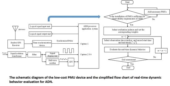
The schematic design diagram of a low-cost PMU device based on the non-DFT method is shown in
Figure 1.
As indicated in
Figure 1, the three-phase voltage-measured signals
uA,
uB, and
uC are being isolated, transformed, and filtered, respectively. Subsequently, only the base-frequency voltage signal is transformed into a DC voltage signal with a small unidirectional ripple by the full-wave rectifier and input to the A/D (analog to digital) conversion module to be processed by the microprocessor further. By sampling the DC voltage signal, the microprocessor can get the average value in the signal period, and then the amplitude of the measured voltage signal is obtained. A simple circuit can implement this method with high precision and small-quantity computation.
The designed full-wave rectifier circuit is shown in
Figure 2a. The operational amplifier is OP07, diodes
D1–
D5 are 1N4007, the value of the input resistance
R1 and the operational amplifier input and output resistances
R2–
R4 are 10 kΩ, while
R5 is 100 Ω. The measured voltage signal
us is rectified into a one-way full-wave rectified voltage signal
usq through an operational amplifier circuit.
usq is the combination of the positive half of us and the phase reversed negative half of
us.
usq is a DC full-wave voltage signal with large pulsations. When the resistive load
R is connected in parallel with a filter capacitor
C, the output voltage
uo, which is originally a full-wave DC voltage waveform with large pulsation, will be smoothed. The pulsation component will be reduced, and the average value of output voltage
uo will be improved, as indicated in
Figure 2b.
The proposed non-DFT-based PMUs device can achieve high-precision measurement of three-phase frequency, phase, and amplitude parameters of voltage and current phasors even when the frequency is offset. It has the advantage of low cost with no need for expensive ADC and microprocessor chips. Thus, it is feasible to widely allocate the PMU devices at each node, enabling the observation and evaluation of dynamic characteristics across the whole distribution network.
For the parameter of the resistor
R and capacitor
C of the above full-wave rectifier-capacitor filter circuit, the values are generally determined according to the following equation.
where
T is the period of the measured voltage signal
us, and the value of
T is 20 ms for the fundamental signal. In the designed circuit, the value of
R is 10 kΩ while the value of
C is 4.7 μF. Assuming that the amplitude of
us is
, the withstand voltage of both the rectifier diode and the filter capacitor should be greater than
.
Assuming that the
N + 1 sampling points before the synchronous measurement time are
f(0),
f(1),
f(2),…,
f(
N − 2),
f(
N − 1),
f(
N), then the sampled average value of output voltage
over one cycle of the measured signal is:
The average value
of the output voltage
after filtering by the full-wave rectifier capacitor conforms to the following equation:
where
is the root-mean-square (RMS) value of the measured voltage signal
.
Thus,
can be expressed as follows:
However, Formula (4) is the ideal relationship between
and
. In practice, the conduction voltage drop of the diode is not zero, so
is not directly proportional to
. In this paper, measured signals of different amplitudes at 50 Hz are simulated, from which the fitted functional relationship between
and
can be obtained as:
Using Formula (5), the measured amplitude
can be calculated. And the measurements and measurement errors of voltage magnitude are displayed in
Table 1. According to
Table 1, when
varies in the range of 3.0~6.0 V, the measured magnitude value
calculated via the fitting function is very close to
, and the maximum relative error of the magnitude value is only 0.17%, indicating the high precision of the magnitude measurements.
Additionally, it can be seen from Formula (4) that the functional relationship between and is relevant to , i.e., it is related to the measured signal frequency fs. In the case where R and C are fixed, the functional relationship between and varies with fs. When fs is 45 Hz and the magnitude ranges from 3.0 V to 6.0 V, the maximum relative error between and is 0.31%; if fs equals 55 Hz, the maximum relative error is 0.42%. It can be observed that the magnitude measurement error becomes larger. In order to decrease the magnitude measurement error, the fitted functional relationship between and should be updated according to the measurements at corresponding fs. In fact, the proposed non-DFT-based PMU can meet 0.5-class smart meter requirements (or even 0.2-class metering device requirements if necessary) when fs varies within 45.0~55.0 Hz.
3. Construction of the Dynamic Index System
3.1. The Guidelines of Online Dynamic Characteristics Assessment of ADN Based on PMUs
Two possible dynamic trajectories of PMU data of ADNs within the observation time window are shown in
Figure 3. Unlike the dynamic process of a second-order control system that always converges, the PMU data of an ADN is in the dynamic process at all times and may never converge. Still, by referring to the definition of the steady-state interval of the second-order control system, we can define the average value of the measurements in the observation time window as “equivalent steady-state value” and furthermore define its “equivalent balance interval”, which will be described in detail in
Section 3.1 and
Section 3.2.
Then, the real-time evaluation guidelines of ADN’s dynamic characteristics are:
- (1)
Scientificity: The adverse dynamic process of ADN can be accurately identified by sufficiently considering the influence of distributed power, energy storage system, electric vehicle charging facilities, flexible load, and control system coupling on the dynamic process of ADN.
- (2)
Integrity: This methodology can estimate the fluctuation of local state variables in the dynamic process of ADN, and simultaneously comprehensively evaluate the dynamic characteristics of subareas and the entire system.
- (3)
Practicability: The evaluation index and model are supposed to be concise and speedy calculated online. The real-time cycle mode is adopted in the evaluation process, which can evaluate the dynamic characteristics of the present object in different time periods.
- (4)
Adaptability: Considering the frequent changes of the operation mode and topology structure of ADN, the assessment method should be capable of conducting real-time evaluation without the information of operating modes, network topology, or line parameters. For instance, while optimizing the dynamic characteristics of ADN by changing its topology or adopting additional control, the evaluation method should reflect the changes of the dynamic indexes before and after taking these measures in time, which can provide the basis for the dynamic characteristics optimization control.
It is worthy of notice that the data collected by PMUs can monitor the real-time dynamic process of ADN. The low-cost PMUs are developed and assumed installed at each node in this paper so that the observability is well implemented in the ADN.
The dynamic index system is built up for the ADN dynamic characteristics evaluation according to the aforementioned guiding ideology. The redundancy of the built-up dynamic index subset is needed taking into account the convenient usage of the dynamic index calculation results and the ability to describe the problem from multiple aspects, which means that some dynamic indexes are correlated or coupled. However, the correct evaluation results of ADN dynamic characteristics can be obtained by selecting a set of irrelevant or approximately irrelevant indicators according to the principle of completeness.
The built-up dynamic index set includes four parts: individual node dynamic index, individual branch dynamic index, subarea dynamic index, and whole network dynamic index, which will be introduced below.
3.2. Dynamic Index of Individual Node Voltage
The objective of the proposed dynamic index of node voltage is involved in two aspects:
- (1)
By computing the dynamic indexes of node voltage amplitude online, it is expected to find out whether the node voltage frequently exceeds the allowed limits in the dynamic process of the ADN, including the amplitude and frequency beyond the allowed limits as well as the percentage of time of the voltage limit violations.
- (2)
By calculating the dynamic indexes of instantaneous frequency and phase angle of node voltage online, it is expected to discover in time whether there are adverse dynamic processes such as periodic oscillation in the ADN.
3.2.1. Dynamic Index of Individual Node Voltage Amplitude
Assuming that the number of the voltage amplitude measurements at the node j in the present observation time window is N (note: the measurements include the data collected at the starting time of the time window t = 0, the sample time interval is , the length of the time window is , the (N + 1)th data (presented by per unit value) can be observed but belongs to the following observation time window), the number of the sampled data point is noted as i, the average value at node j is and expressed as , the corresponding “equivalent balance interval” is , the node rated voltage is and its rated voltage magnitude is expressed as , the normal range of is . Seven dynamic indexes to evaluate the changes of node voltage amplitude over the observation time are proposed and introduced as follows.
- (1)
Percentage of voltage regulation time and Percentage of voltage over-limit time
Definition and Calculation 1. The percentage of the node voltage amplitude regulation time refers to the percentage of data points whose relative error of the voltage amplitude measurement value to the average voltage measurement value is more than 2% in the present observation time window. Set NAT as the number of the data points of voltage magnitude measurements beyond the “equivalent balance interval” in the present time observation window, then the voltage amplitude regulation time percentage at node j in the present observation time window is: Similarly, the percentage of time that the node voltage exceeds the limits can be defined.
Definition and Calculation 2. The percentage of the voltage over-limit time refers to the percentage of data points whose voltage amplitude measurement values are in the over-limit state in the present observation time window. Let NET represent the number of the data points of voltage magnitude measurements beyond the normal range over the rated voltage in the present time observation window. Thus, the voltage amplitude over-limit time percentage at node j in the present observation time window is calculated as follows: - (2)
Maximum fluctuation of voltage amplitude and maximum over-limit degree of voltage amplitude
Definition and Calculation 3. The maximum fluctuation of voltage magnitude refers to the percentage of the difference between the maximum voltage measurement and minimum voltage measurement over the average voltage measurement. Assuming that the sampled data point number is labeled as i or l. The maximum fluctuation of voltage magnitude at node j in the present observation time window is written as: Definition and Calculation 4. The maximum over-limit degree of voltage amplitude refers to the maximum percentage of the value of the voltage magnitude measurement deviated from the normal range over the rated voltage, and is calculated as follows: - (3)
Voltage amplitude discrete intensity and Voltage over-limits intensity
The closer the node voltage amplitude dynamic trajectory is to the average value in its observation time window, or the closer it is to the upper and lower voltage bands, the better its dynamic characteristics. Based on this, this paper comprehensively considers the information of the two dimensions of amplitude and time and proposes two indicators as follows.
Definition and Calculation 5. The voltage amplitude discrete intensity at node j in the present observation time window is displayed as follows: Definition and Calculation 6. The voltage amplitude over-limit intensity at node j in the present observation time window is displayed as follows: - (4)
Percentage of voltage amplitude fluctuation frequency
In dynamic systems, small inertia indicates that the state variables are prone to fluctuations. Considering this, in order to evaluate the “inertia” of the ADN, this paper defines the index of the percentage of voltage amplitude fluctuation frequency during the observation time window.
Definition and Calculation 7. Percentage of voltage amplitude fluctuation frequency refers to the percentage of the actual total times for which the voltage amplitude curve crosses the “equivalent balance interval” over the theoretical maximum crossing times.
Based on the discrete voltage amplitude measurements at node
j in the present observation time window, the number of times the voltage amplitude dynamic trajectory traverses equivalent balance interval is recorded as
NUP, then the voltage amplitude fluctuation frequency percentage at node
j in the observation time window is described as
To calculate the value of
NUP in (12), the classification function
Usj is defined as
The calculation method of
NUP is summarized in Algorithm 1.
| Algorithm 1 The Calculation Method of NUP |
| 1: Initialize i = 1, NUP = 0 |
| 2: while i ≤ N − 1 do |
| 3: if then |
| 4: NUP = NUP + 1; |
| 5: i = i + 1; |
| 6: end if |
| 7: end while |
| 8: Output NUP = NUP. |
3.2.2. Dynamic Index of Individual Node Voltage Phase
The main grid is approximately regarded as an infinite system considering the ADN is connected to it through transformers and high-voltage distribution lines. Therefore, when the load or the DG output changes significantly in the ADN, the voltage phase of the related node will accordingly change non-steady at the same time. The non-steady voltage phase change described here is in terms of the steady phase change relatively.
The steady change of node voltage phase is defined as: in a relatively long length of the observation time window, the present angle frequency of node voltage is obtained based on the frequency measurement data acquired by the PMUs, and the data sampling time interval is set as , then the steady change of node voltage phase is represented as . Thus, if the voltage phase data at one node acquired by PMUs is deviated from beyond the set threshold, it is said that the voltage phase at this node occurs non-steady change.
It is indicated that the loads or DG outputs experience frequent impacts if the bus voltage phase often appears relatively significant non-steady changes. The more significant the impact is in the observation time window, the worse the dynamic characteristics of the ADN. On the other hand, if there is active power oscillation in the ADN in the observation window, the corresponding node voltage will occur non-steady change periodically. This kind of periodic non-steady change will also arise the periodic change of the voltage phase differences between different nodes.
Based on the aforementioned analysis, two indexes, i.e., the degree of voltage phase non-steady change and the maximum swing of voltage phase difference, are defined to indicate the impact loads and DG outputs as well as the degree of the active power oscillation in the ADN. Assume that there are N measurements for the voltage frequency and absolute voltage phase at the node j in the observation time window, and the sampled data point number is noted as i, then the definition and calculation methods of these two indexes are as follows.
- (1)
Degree of voltage phase non-steady change
Definition and Calculation 8. The average frequency is represented by , and the steady change of the node voltage phase is marked as . When the voltage phase changes within the range , it is inferred that no non-steady change occurs. Thus, the degree of voltage phase non-steady change at node j in the observation time window is: - (2)
Maximum swing of voltage phase difference
Definition and Calculation 9. It is assumed that the node with the minimum value of the non-steady change degree in the whole network is numbered as s. Refer to node s, the voltage phase difference between node j and node s is represented as . Thus, the maximum swing of voltage phase difference at node j in the present observation time window is described as follows. 3.3. Dynamic Index of Individual Branch
The most basic operating variable of a branch is current, but its power more intuitively describes the dynamic characteristics. Therefore, when defining the branch dynamic indexes, the focus is on the current amplitude over-limit situation and the power fluctuation situation during the dynamic process. Simultaneously, to evaluate the dynamic compensation capability of the reactive power compensation device and the reactive power adjustment function of DGs in ADN, a dynamic index regarding the branch power factor is proposed. Most of the definitions of branch dynamic index can be given by referring to node voltage dynamic indexes, which will not be repeated in this section. It should be noted that there may be bidirectional power flow in ADN, and the measured value of the backward power flow is expressed as minus, as shown in
Figure 3b.
Assuming that the numbers of measurements of the current amplitude Ik, the active power Pk, the reactive power Qk and the power factor Fk of branch k in the observation time window are N. The sampled data point number is noted as i. The average values of these four kinds of measurements are , , , , respectively. The power limit of branch k is expressed as . Then the indexes of branch k in the observation time window are:
- (1)
Maximum over-limit degree of current
- (2)
Current over-limit intensity
- (3)
Percentage of current fluctuation frequency
Definition and Calculation 10. Percentage of current fluctuation frequency refers to the percentage of the actual total times for which the current curve crosses the “equivalent balance interval” over the theoretical maximum crossing times.
Considering the bidirectional power flow, the average value of nonnegative measured values is recorded as
, and the average value of negative measurements is denoted as
. For dramatic fluctuation of branch current, the corresponding “equivalent balance interval +” is set as
, while the “equivalent balance interval −” is set as
. Based on the discrete current measurements of branch
k in the present observation time window, the number of times the current dynamic trajectory crosses the “equivalent balance interval (including the equivalent balance interval + and the equivalent balance interval −)” is recorded as
NIP, then the percentage of current fluctuation frequency of branch
k in the observation time window is:
The calculation method of NIP is similar to NUP, but the influence of the positive and negative measurement value needs to be considered as follows:
First, define the classification function
as:
Apply
to clarify elements in
one by one and obtain the one-dimensional classification vector
. Then the value of
is as below:
- (4)
Active/Reactive power discrete intensity (
X =
P or Q)
3.4. Dynamic Comprehensive Index
After calculating each node’s voltage dynamic index and each branch’s dynamic index, the dynamic comprehensive indexes of node voltage and branch in the subareas and the whole ADN can be obtained.
- (1)
Dynamic comprehensive index of subareas
According to the statistics of the dynamic indexes of all nodes in this subarea, the maximum and average values of the non-zero indexes are defined as two kinds of dynamic comprehensive indexes of the nodes, as shown in
Table 2. Assuming that the total number of nodes in the present subarea is
J. Taking the comprehensive index corresponding to
UATj as an example, it is suggested that the voltage amplitude regulation time percentage of each node has been calculated and recorded in a one-dimensional vector
UAT = (
UATj)
J×1, and the total number of non-zero elements in
UAT is
M. The set of these
M nodes is represented by
Mnode, then the corresponding two types of subarea dynamic comprehensive indexes are shown as follows.
If the value of an index at all nodes in this subarea is zero, then Mnode is an empty set, and the corresponding maximum index and average index are both zero.
Similar to the node voltage dynamic comprehensive index, two types of dynamic comprehensive indexes of the branch dynamics in subareas can be defined, as shown in
Table 2.
- (2)
Dynamic comprehensive index of the whole network
For the whole network, there are also two categories of dynamic comprehensive indexes, i.e., the maximum category and the average category, as presented in
Table 2. The calculation method of these indexes is similar to the subareas indexes.
According to
Table 2, there are 30 indexes in the subareas evaluation index system and the whole network evaluation index system, respectively, which can be used to diagnose over-limit, short-time impact, and oscillation. The value of these indexes can characterize the severity of the corresponding adverse dynamics. All indexes’ values range between [0%, 100%] and can be compared mutually. In practical application, the corresponding set of indexes can be flexibly selected according to the assessment needs. This is the reason for constructing a ‘redundancy’ index system.
5. Case Study
In order to verify the practicability and effectiveness of the proposed dynamic characteristic evaluation method, a numerical test is carried out on the modified IEEE 123-bus distribution network shown in
Figure 5. This system has 123 nodes and 122 branches, which is comparable to a real regional distribution network. The voltage magnitude of the substation bus is set to be 10.5 kV as a reference, and the upper and the lower voltage limits for each bus are set to be 1.05 p.u. and 0.95 p.u., respectively. The network is partition into three subareas based on the distance to the reference node, with subarea 2 being the EV charging zone and subarea 3 being the DG demonstration zone. Both EV charging stations and DGs have two types and are labeled separately. In this paper, all DGs and loads are simulated as having a constant power factor.
The installed capacities of DG-1 to DG-7 are 0.5, 1.3, 0.68, 0.48, 1.42, 0.71, 1.08 MW, respectively. The forecasting output of each DG unit is 50% of the installed capacity, and the random forecasting error fluctuates according to the Laplace distribution, within the limit of [0, installed capacity]. Based on the DG output as the benchmark and changing the standard deviation of Laplace distribution, two types of actual DG output curves can be obtained, as shown in
Figure 6a. For buses with uncertain load, the corresponding actual load demand curves with the benchmark of the standard load are obtained as shown in
Figure 6b. According to the results in
Table 1, the error of PMU measurement data is set to be 0.2%. The error is modeled as Gaussian variance and added to the measurements. The other detailed parameters of the network are from references [
26,
27].
5.1. Online Dynamic Characteristics Assessment in a Single Time Window
Assuming that there is one sampling point in one frequency period, the observation time window length is 2 s. According to the flow shown in
Figure 4, indicators are selected to construct the subsets of the over-limit index, oscillation index, and short-time impact index, and the dynamic characteristics indexes of the whole network in the 1st time window are solved and listed in
Table 3.
Among them, the maximum values of indexes {, } appear at bus {43, 115}, respectively. The maximum values of indexes {, } appear at branches {14–119, 1–2} (if the maximum value of index appears at multiple nodes or branches, the minimum number is counted as the solution). Combined with the above information, the analysis is shown as follows:
- (1)
The value of indexes in the over-limit index subset are zero, so there is no over-limit situation in the network in the 1st time window.
- (2)
Check the values in oscillation index subset and short-term impact index subset. For the dynamic index of node voltage, the maximum value of comes from bus-43, reflecting the influence of the impact loads around; the maximum value of appears at bus-115, indicating that this index is mainly affected by the fluctuation of DG-6 output. For branch dynamic indexes, occurs in branch 14–119, while appears in branch 1–2, both reflects the variation of the power delivered from this branch to the nodes behind.
- (3)
CI of the whole network is 10.1084, which indicates that the dynamic characteristics of this network in the present time window is relatively acceptable but can still be optimized.
5.2. Online Dynamic Characteristics Evaluation on Moving Time Window
The dynamic characteristics of this distribution system are evaluated in 10 consecutive moving time windows with the step length of 1 s. The over-limit index subset, oscillation index subset, and short-time impact index subset are consistent with
Section 5.1. The numerical curves of some typical indexes (including subarea indexes and the whole network indexes) are plotted in
Figure 7, which show that:
- (1)
The comprehensive dynamic characteristic index for the whole network is influenced by the coupling of the three zones with each other, and always follows the worst situation among subareas.
- (2)
The non-zero values of over-limit index and short-time impact index , all appear in the last two time windows. It is clear that the former two follow the impact in subarea 2, while the latter one comes from subarea 1. However, appears at branch 1–2 during the entire observation period, which reflects the electricity from utility grid to this network to satisfy its load demand. Thus, the non-zero values of all these three indexes are due to the influence of load impact in subarea 2.
- (3)
is not zero but remains zero in the first eight time windows. A comparison of these two indexes shows that the fluctuations of in the first eight time windows are mainly due to the bidirectional power flow caused by stochastic DG output. However, this fluctuation does not result in the over-limit of current. Comparing the values of and together with their changes leads to the same conclusion.
- (4)
The value of CI increases significantly in the 9th time window, reflecting the influences of the impact loads at subarea 2. It then decreases slightly in the 10th time window, which, combined with the fluctuating trend of , can be seen as a result of the fluctuation of DG output slowing down in the 10th window.
The assessment results in different subareas of the modified IEEE 123-bus network show that the proposed assessment method is not dependent on a particular topology or a particular operation mode of the active distribution network and is highly adaptable. Moreover, it is worth noting that for ADN in large zones, the comprehensive dynamic characteristic index for subareas can quickly suggest areas where adverse dynamic triggers are likely to be located.


