Estimation of Heat Loss Coefficient and Thermal Demands of In-Use Building by Capturing Thermal Inertia Using LSTM Neural Networks

Abstract

Accurate forecasting of a building thermal performance can help to optimize its energy consumption. In addition, obtaining the Heat Loss Coefficient (HLC) allows characterizing the thermal envelope of the building under conditions of use. The aim of this work is to study the thermal inertia of a building developing a new methodology based on Long Short-Term Memory (LSTM) neural networks. This approach was applied to the Rectorate building of the University of Basque Country (UPV/EHU), located in the north of Spain. A comparison of different time-lags selected to catch the thermal inertia has been carried out using the CV(RMSE) and the MBE errors, as advised by ASHRAE. The main contribution of this work lies in the analysis of thermal inertia detection and its influence on the thermal behavior of the building, obtaining a model capable of predicting the thermal demand with an error between 12 and 21%. Moreover, the viability of LSTM neural networks to estimate the HLC of an in-use building with an error below 4% was demonstrated.

1. Introduction

The building sector is one of the largest energy consumers in the European Union, representing more than 40% of the total energy consumption, with the associated greenhouse gases emissions responsible for near 36% of total emissions [1]. From this energy, more than 50% is consumed by HVAC (Heating, Ventilation and Air Conditioning) systems [1]. In this context, several institutions have established guidelines and directives to improve energy efficiency of buildings, fixing an objective of nearly zero-energy buildings (nZEB). To achieve this goal, the European Union, through the strategic program Horizon Europe, is driving new initiatives, such as creating more than 100 climate-neutral cities by 2030 [2].

However, both actual buildings that are already designed to achieve this nearly zero emissions objective and retrofitted buildings are failing during the process [3]. This is because there is still a difference between real and theoretical performance that, in certain occasions, even reaches from two to five times the design energy consumption [4,5,6]. This difference is commonly called performance gap. Different technologies have been developed to reduce energy consumption and narrow this gap. Physics-based tools (also called white-box models) such as dynamic simulation can help to make decisions about the best measures to reduce energy demand and improve indoor thermal comfort [7,8,9]. However, the assignment to attain accurate simulation models can be complex as it depends on many variables and parameters [10,11].

On the other hand, district heating system (DHS) constitutes an often used solution in the northern and the central-European cities and it is gaining presence in Spanish cities such as Bilbao and Barcelona [12]. DHS is a building arrangement designed to generate and store energy in a centralized location to later distribute it to the network of buildings according to demand [13]. The main difficulty of this system, in addition to its dimensioning, is to adjust the operation to avoid over-production or under-production of energy. The balance between the heat production and the heat demand leads to a reduction of emissions and an improvement in the system efficiency as a whole [14].

Under these circumstances, the use of data-driven tools (commonly known as black-box models) have been consolidated as a flexible and efficient tool to achieve accurate predictions [15,16,17]. The requirements to construct appropriate models consist of an adequate structure and a healthy dataset (i.e., no empty fields or useless data) [18]. The application of the technology of Internet of Things (IoT) provides a lot of information about the building conditions that can be especially useful to characterize its functions and construct a wide variety of scenarios [19,20].

However, forecasting heat demand implies dealing with a complex nonlinear problem influenced by multiple factors such as weather conditions and thermal inertia of the building. This term, applied to a building, means property that expresses the degree of slowness with which its (indoor temperature in this case) temperature reaches that of the environment (outdoor temperature). In this context, Long Short-Term Memory neural networks (LSTM), a variation of deep Recurrent Neural Networks (RNN) originally developed by Hochreiter et al. [21], provides a reliable option for modelling this type of sequential data. This variety of neural network includes an internal structure designed to deal with gradients and is especially useful to catch systems inertia.

In connection with this, HLC is introduced as one of the most useful Key Performance Indicators (KPI) to characterize the building envelope energy efficiency. The envelope of the building cannot maintain the same thermal efficiency in hot seasons as in cold seasons; it always produces a loss of heat in winter and a gain in summer. Through HLC, the rate of heat flow between indoor and outdoor air when a temperature difference exists is determined. Using forecasting results from neural network avoids dealing with physical building simulation, which requires the precise description of elements that compose the thermal envelope of the building (insulation, wall thickness, etc.).

The aim of this work is to develop a methodology based on LSTM neural networks to identify the building thermal inertia and obtain a precise prediction of building thermal demands which will be used to estimate the HLC. This process will be applied to the Rectorate building of the University of Basque Country (UPV/EHU), located in the north of Spain, but the method could be used in other locations and climates, since it is only necessary to know the temperature and radiation in the location of the building under study. The dataset consists of hourly observations of indoor (temperature, relative humidity, and CO₂ concentration) and outdoor variables (temperature, relative humidity, and solar radiation). The accuracy of the models developed is quantified using the Coefficient of Variation of the Root Mean Squared Error (CV(RMSE)) and the Mean Bias Error (MBE). These error measures were both recommended by the American Society of Heating, Refrigerating and Air-Conditioning engineers (ASHRAE) and validated on Guideline 14 [22].

2. Materials and Methods

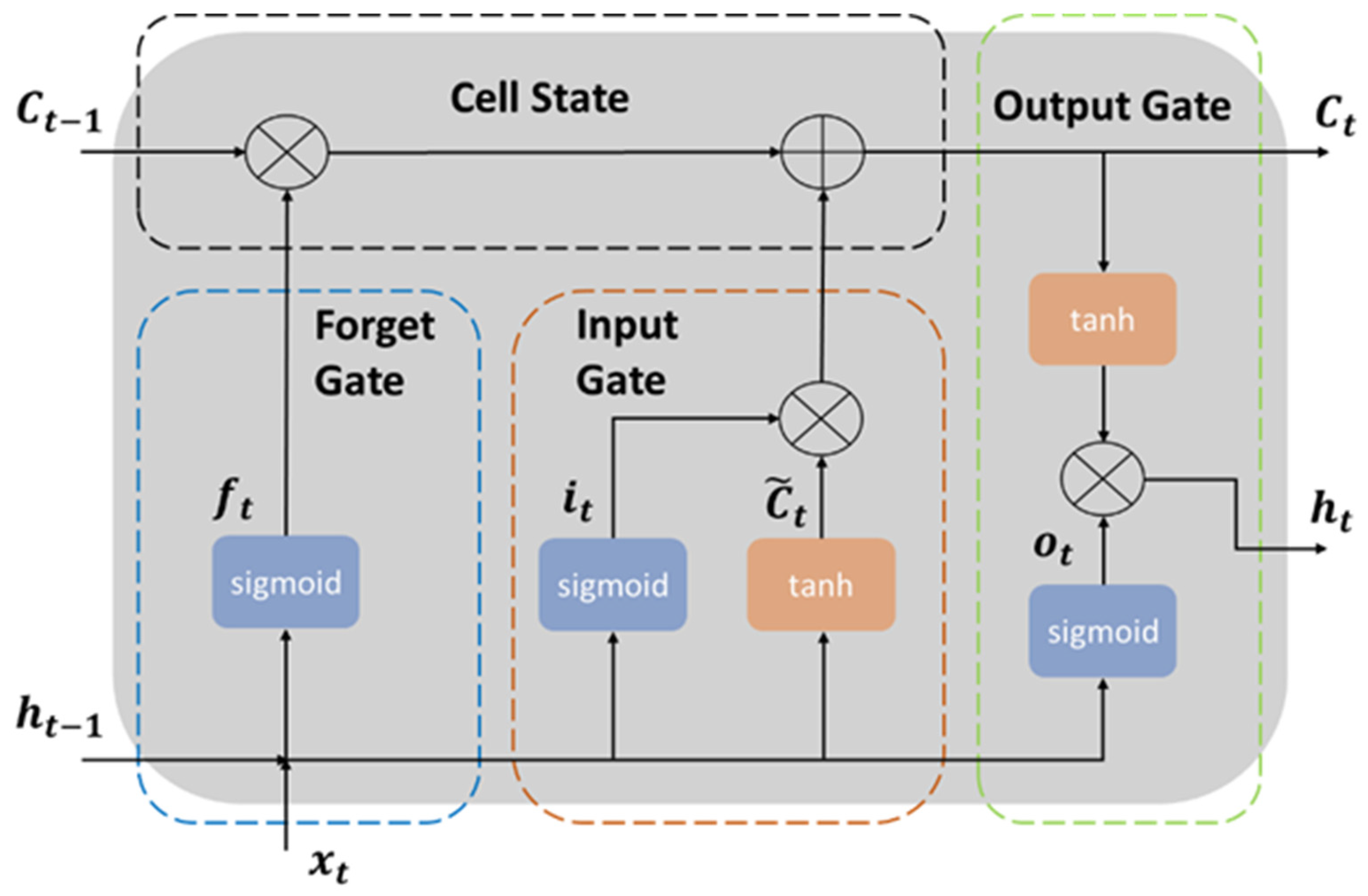
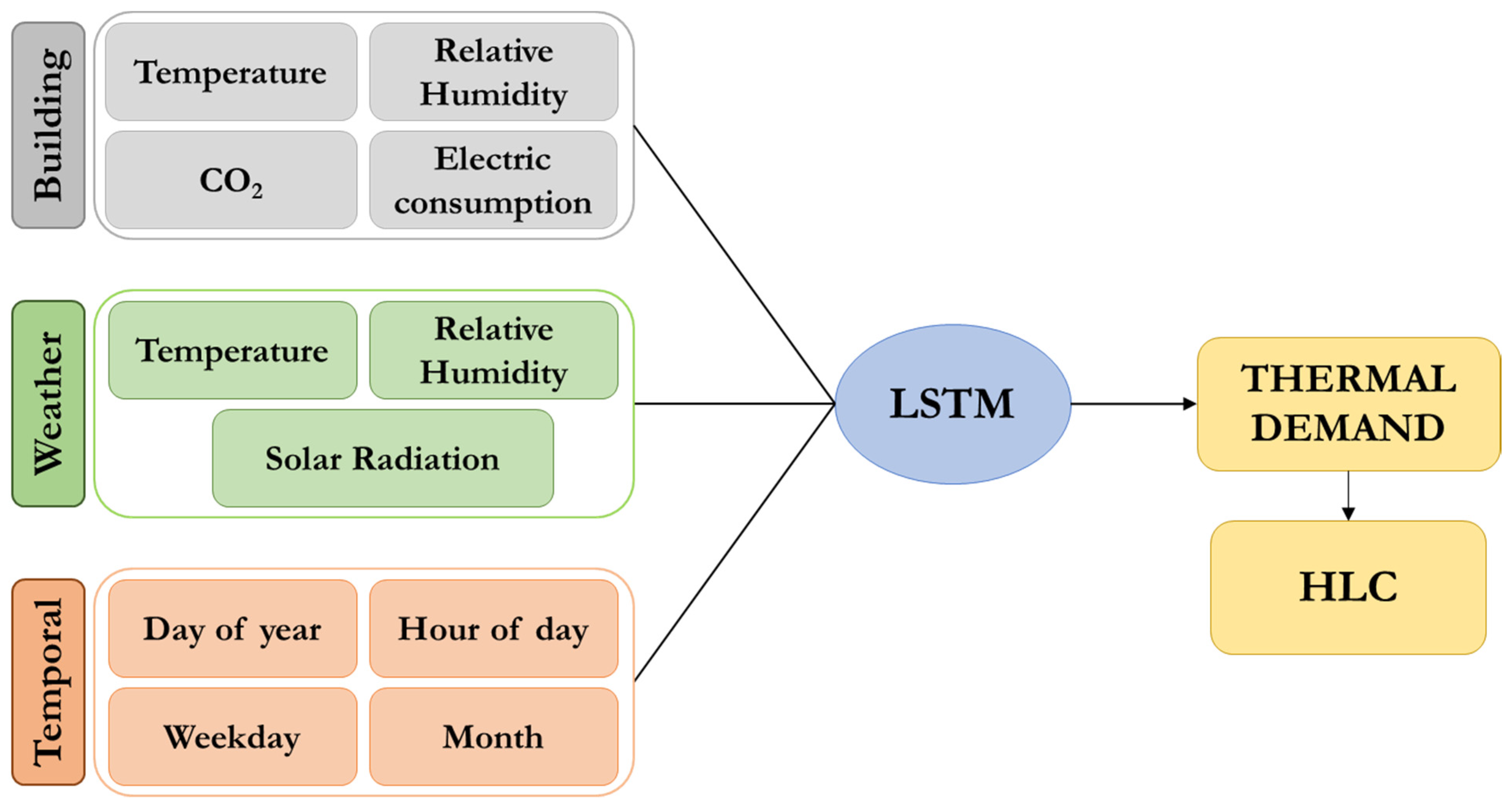
2.1. LSTM Architecture

Long Short-Term Memory (LSTM) is a variety of Recurrent Neural Network (RNN) architecture created to avoid the problem of the vanishing (or exploding) gradient that classic RNN presents when using back propagation. LTSM is characterized for being able to learn long-term dependencies, which allows it to model time sequences more accurately than conventional RNNs. These characteristics make it a very appropriate approach to long-term dependency problems. The solution presented by LSTM cells is based on its gates and how each affects the information that comes from the cell state. Figure 1 shows the different gates of the cell.

Sigmoid and tanh (Figure 1) are activation functions used in neural networks to define how the weighted sum of the input is transformed into an output from a node or nodes in a layer of the network.

The key on LSTM neural networks is the cell state. This cell is updated every time step based on the input gate, the forget gate and the output gate. The input gate determines how much new information is stored on the cell state. The forget gate decides how much information will drop out the cell state. The output gate selects which information will be sent out the cell state. Through the dynamic interaction of these gates with the coming information over the cell state, LSTM neural networks are capable of retaining information for many time steps. LSTM input structure is a three-dimensional array. The meaning of the three input dimensions are samples, time-lags and features. The time-lags denote the number of previous time steps considered to obtain the prediction. Each sample contains x time-lags so, for example, on a 1000 row dataset, with a time-lag of 10, we will have 100 samples. Depending on the number of time-lags selected the neural network structure will be different, because while incrementing the time-lags, the amount of information to process raises, which makes it necessary to adapt the layers’ structure. This configuration will be discussed in Section 3.3.

2.2. Heat Loss Coefficient (HLC)

The Heat Loss Coefficient (HLC) is an indicator of the performance of a building envelope. It represents the rate of heat flow through a building’s envelope when indoor and outdoor temperatures differ. The method used in this work to obtain the HLC was described by Uriarte et al. [23].

$$HLC=\left(UA+C_v\right)=\frac{\left(Q+K\right)+S_a{V}_{sol}}{T_{in}-T_{out}} \left[\frac{kW}{K}\right]$$

(1)

In the Equation (1) HLC represents the addition of the two coefficients, one that represents the heat losses through the whole building envelope (UA) and a second that means the infiltration heat losses ($C_v$). On the right part of the expression, Q are all energy inputs of the building (heating and ventilation systems) [kW], K includes passive heat gains, such as lighting and heat due to occupation (metabolic heat gains) [kW], $T_{in}-T_{out}$ is the difference between indoor and outdoor temperature [K] and $S_a{V}_{sol}$ represents the solar radiation heat gains of the building.

In this work, to obtain the HLC, the right part of the expression was used. The equation presents terms difficult to obtain (e.g., the solar gains). In addition, the requirement of stationary conditions represents an additional issue when measuring the HLC of in-use buildings.

To simplify this characterization, the component that includes the solar radiation heat gains was not considered, this way obtaining the HLC simple. The requirement to apply that simplification is to search for periods when solar radiation is below 10% of the rest of the heat gains.

In order to have a reference to compare the results, periods 4 and 5 presented by Uriarte et al. [23] were used to evaluate the precision of the results. Then, a third period was selected to extrapolate the application.

2.3. Validation and Error Measurement

The performance of the forecast techniques applied in this article are measured using the Coefficient of Variation of the Root Mean Squared Error (CV(RMSE)) and the Mean Bias Error (MBE). CV(RMSE) is the RMSE, normalized by the mean of the measured values. On the other hand, MBE detects if the model is producing an overestimation (MBE < 0) or an underestimation (MBE > 0) and its magnitude. Both measurements are referred to in Equations (2) and (3), respectively:

$$CV\left(RMSE\right)=100·\frac{1}{\overline{Y}}\sqrt{\frac{{\sum }_{i=1}^N{\left(Y_i-{\widehat{Y}}_i\right)}^2}{N}}$$

(2)

$$MBE=\frac{{\sum }_{i=1}^N\left(Y_i-{\widehat{Y}}_i\right)}{{\sum }_{i=1}^N\left(Y_i\right)}$$

(3)

where N is the number of samples, Y is the real value, $\overline{Y}$ is the mean of the measured values and $\widehat{Y}$ is the predicted value.

The CV(RMSE) was used to select the best model on every validation iteration. This error is also used to determine if the model is calibrated, based on the criteria established by the ASHRAE in Guideline 14, according to which a model is calibrated if CV(RMSE) is below 30% hourly.

Both errors were used to compare the different models with the test samples.

3. Experimental Case of Study

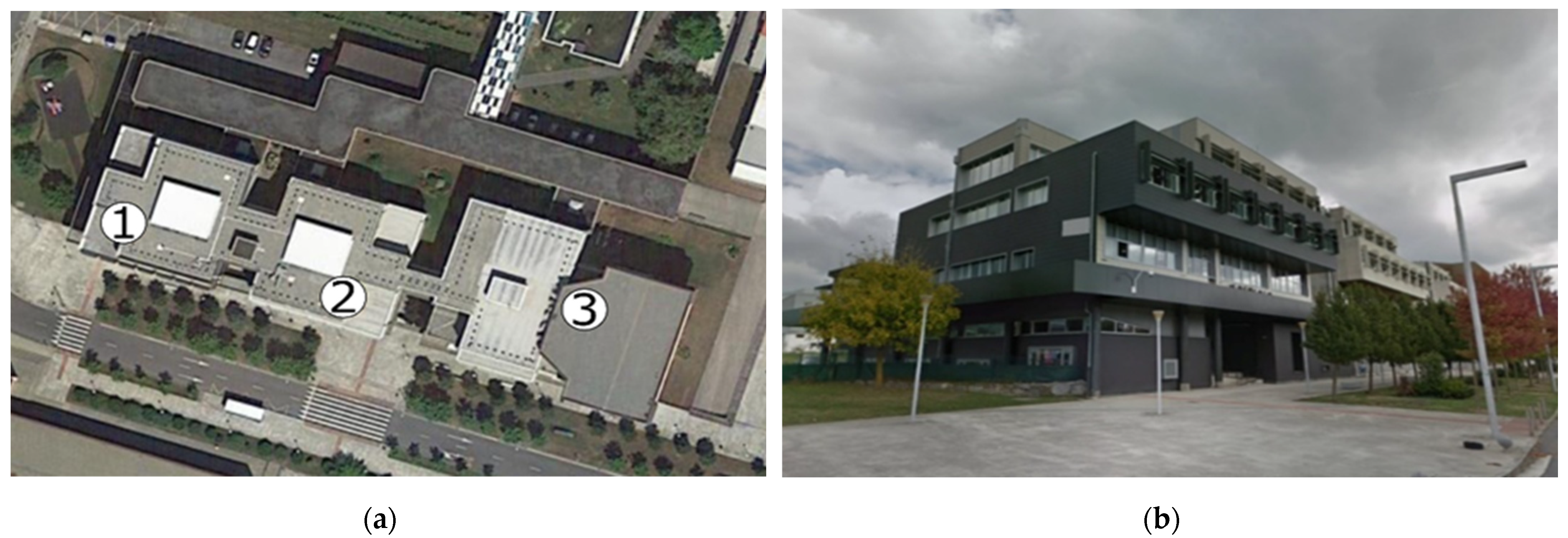
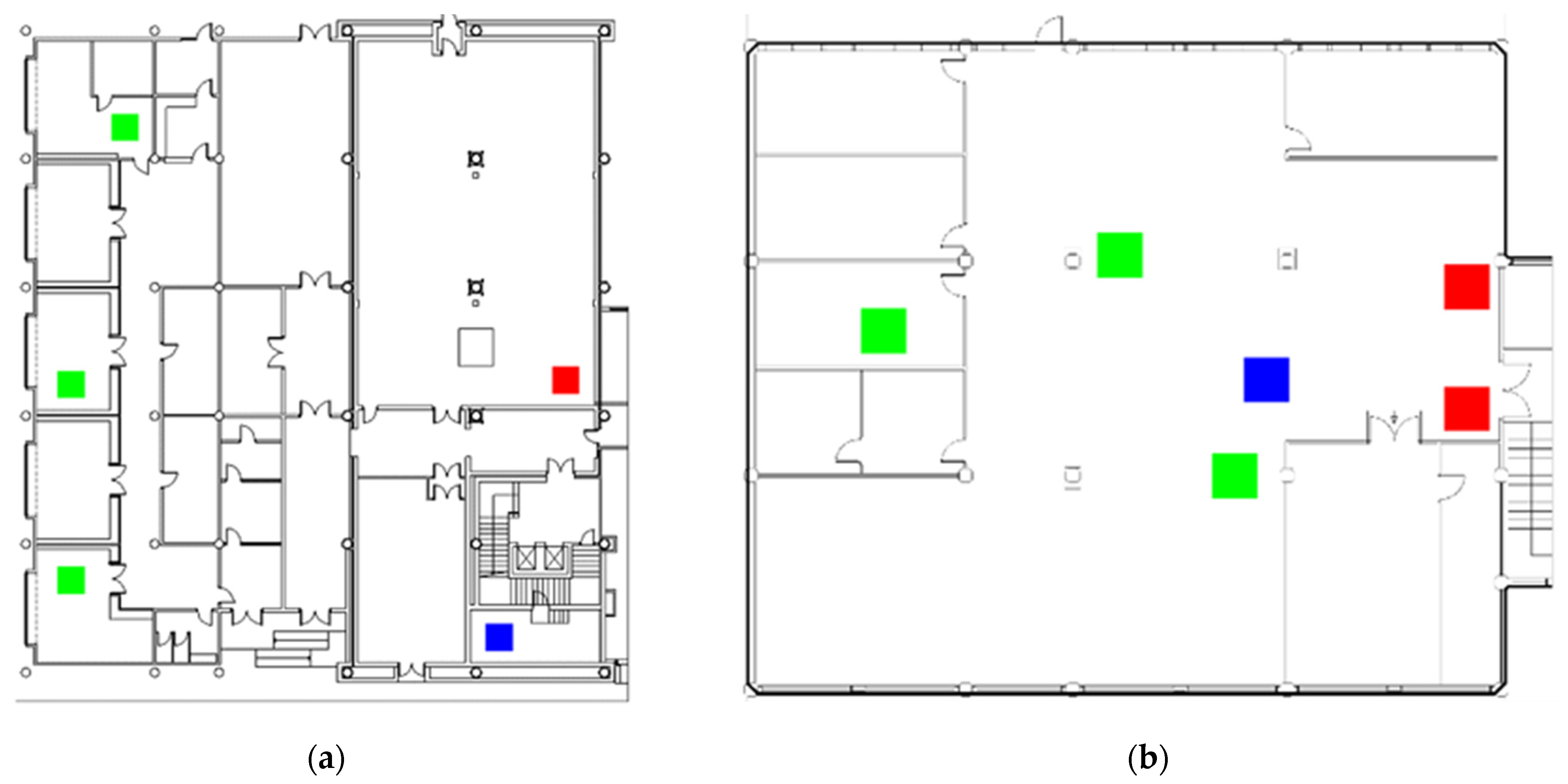
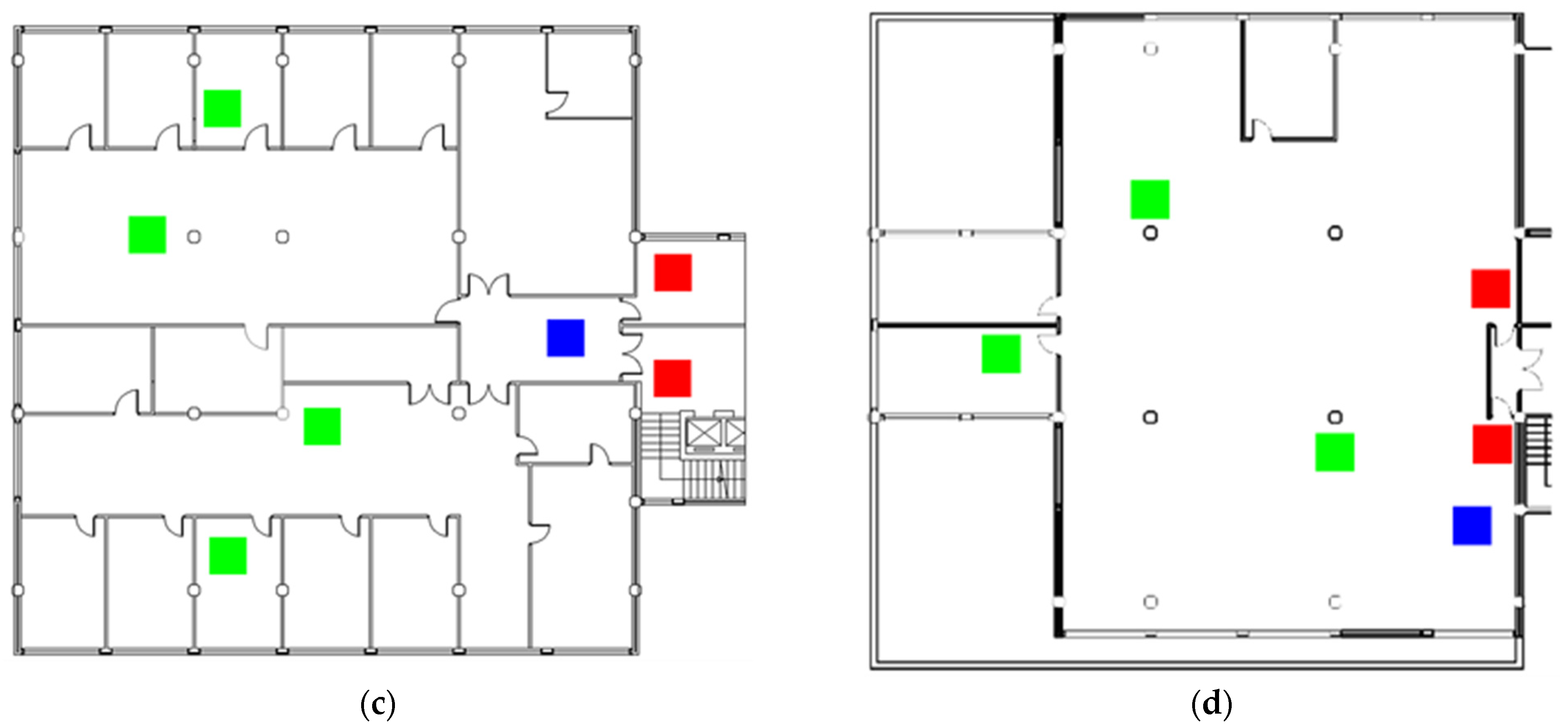
3.1. Building and Heating System Description

The case of study of this work is the Rectorate building of the University of the Basque Country (Spain). The building consists of three blocks, west, central, and east, as shown in Figure 2a. The building was constructed in the 1970s and it was refurbished in the summer of 2016 on the ground floor and in the summer of 2017 in the rest of the building to reduce its energy consumption. The actual façade is shown in Figure 2b. More information about the refurbishment is detailed in [23].

The west block was the only block considered. It is an office building, and the ground floor includes a nursery. It has four floors; on one hand, the Ground Floor (GF) and the Second Floor (2F) consist of rooms, on the other hand, the First Floor (1F) and the Third Floor (3F) are mainly open spaces. It is occupied only during weekdays, being reduced during summer.

A centralized campus district heating system provides heat to the building heating system to meet its heating loads. This heat is managed by a centralized system and distributed by hot water radiators. The heating works the whole year following a control program according to a schedule from 6 a.m. to 7 p.m. except in July and August, when the heating remains off [24]. There was no air conditioning system operating during the studied period.

The monitored variables include outdoor conditions, indoor conditions and building heating. Indoor conditions are monitored by several points of the floor while electrical consumption and heating consumption are provided per floor. Figure 3 shows the sensor distribution for each floor.

More information about the building monitoring system can be found in the work carried out by Erkoreka et al. [25].

Outdoor conditions come from two sources. The first source is the building itself, which includes a set of sensors to measure weather conditions, but only temperature, relative humidity and solar radiation have been considered. The second source is a weather station C039-Deusto (Longitude: −2.99932—Latitude: 43.3463) located at 2.5 km straight line from the building. This source was used to fill long “gaps” on the first source. The meteorological data tables have been obtained with a ten-minute frequency.

3.2. Pre-Processing Data

The data used to train the model were observations between 29 November 2018 to 31 May 2019 while for the validation, the period was from 15 June 2018 to 11 February 2018, for the variables indicated in Figure 4. In the case of building data, the values were obtained using the mean value of the sensors placed on the floor, except for the electricity consumption. Weather data was resampled to obtain hourly frequency values. Time variables are extracted from the date of measurements. In this category, the hour of the day and the weekday are used to catch the influence of the weekday schedule while the month and the day of the year are used to add information about the moment of the year. Four categorical variables were also created to represent the season.

Due to the way LSTM works with time delays, it was necessary to have a continuous sample, without large missing values. There are “outliers” and “gaps” in the building dataset due to sensor errors. “Outliers” have been identified using the values listed in

Table 1. Filters applied to the dataset values.

Variable	Lower Filter	Upper Filter
Indoor TA	15 °C	32 °C
Indoor RH	0%	100%
CO2	200 ppm	1000 ppm
Elec. consumption	25 W	5000 W
Outdoor TA	−15 °C	45 °C
Outdoor RH	0%	100%
Radiation	3.5 W/m2	1500 W/m2

as a filter and they have been replaced by “gaps”. Subsequently, the “gaps” have been filled by second degree polynomial interpolation, for a maximum of three consecutive “gaps”. The same proceeding was applied to the weather dataset.

Through this process the percentage of missing values has been reduced by approximately 12.2%.

3.3. Neural Network Setup

In the case of the thermal demands of the building, the demand for the next hour depends not only on the current state of the building but also on what it had hours ago. This allows the network to differentiate between a building heating or cooling cycle or temperature stabilization, hence, a model based on LSTM is a good choice to predict the heat demand [16]. This inertia is captured using the time-lags previously described in Section 2.1. To catch the thermal inertia of the building, a preselection of the time-lags was developed. A set of time-lags of 3, 6, 12 and 24 h have been simulated to determine which one is the most suitable for this building. In parallel with this, each time-lag selection has a different neural network architecture, changing the relation between the number of LSTM layers and hidden layers. The relations of LSTM-hidden layers were 3-2, 4-2, 5-3 and 5-4. These relations were based on the work carried out by Martínez et al. [16].

The rest of the hyperparameters of the network were tested using a grid to determine the optimum for each floor. The number of neurons in the hidden layers were 50, 100 and 150. The number of epochs was stablished to 100, 150 and 300. To prevent overfitting problems, the network was trained with an early stop parameter of 20% of the maximum epochs, defined using “patience” (limit of epochs without any performance improve).

Moreover, the activation function set was Rectified Linear Unit (ReLU) [26]. The kernel initializer was normal, the optimizing algorithm was the Adaptive Moment Estimation (Adam) [27] and the batch size was equal to 64 [28].

4. Results and Discussion

4.1. Time-Lag Selection

This section compares the results of several trainings to determine the influence of the time delay on the capture of the building thermal inertia. An optimized neural network was applied for each floor, changing only the time-lag. Results are shown on

Table 2. Error comparison of the time-lag change using CV(RMSE) [%].

Time-Lag	GF	1F	2F	3F
3 h	42.43	15.54	28.39	22.64
6 h	39.74	14.37	19.94	20.65
12 h	21.12	12.71	15.92	19.50
24 h	33.95	13.13	20.19	25.32

.

Results show that a low time-lag makes it difficult for the network to capture the inertia, while as it increases the error trends to be lower. This is notable in the fact that the results obtained with a time-lag of 3 h, with the exception of the 3F, has the largest error. It is worth noting the case of the 3F, which differs from the rest by presenting the largest error for the 24 time-lag. This may be caused due to the fact that this floor is the most sensitive to the influence of changes in solar radiation, adding greater variability due to weather changes.

Practically for all floors, time-lags of 6 and 12 h are those with the lowest error. On this, it should be noted how the difference in the error between the interval of 3 and 6 h for the GF is very low, in contrast to the rest. This result suggests that this floor has a larger inertia than the others, which may be caused by better insulation.

It is remarkable how the changes in the time-lag have less effect on the results of the 1F, while for the GF the choice of 12 h as time-lag value manages to halve the error provided by the result obtained using 3 h. This implies that the 1F maintains a more stable situation than the rest over time.

Based on the CV(RMSE) result for every floor changing the time-lags used to estimate the heat demand, the best result is provided in the model with a time lag of 12 h. Additionally, results for 6 h and 24 h delay have good results, while for 3 h the model does not have enough information of the building conditions, i.e., the model does not capture the heating and cooling cycles of the building.

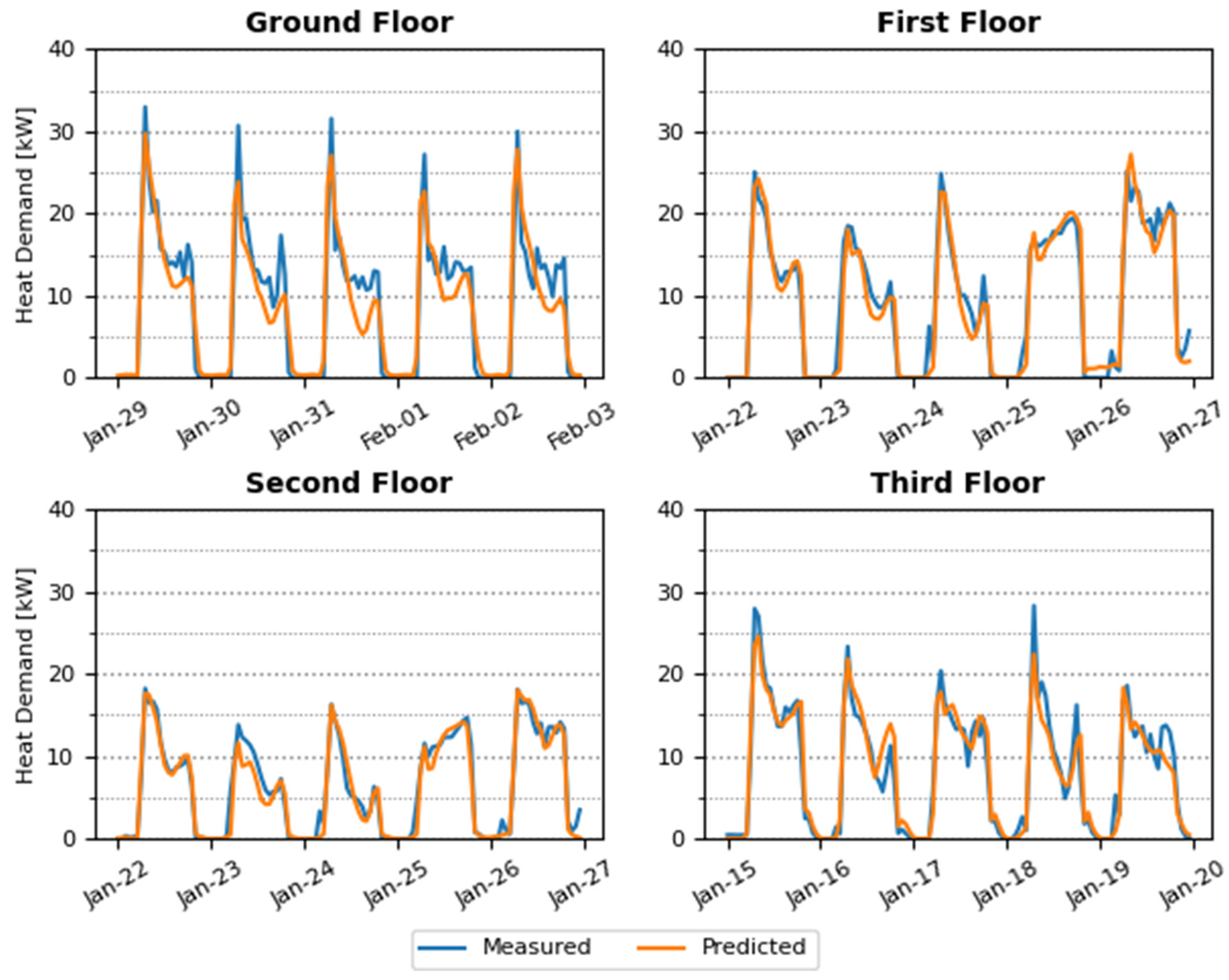
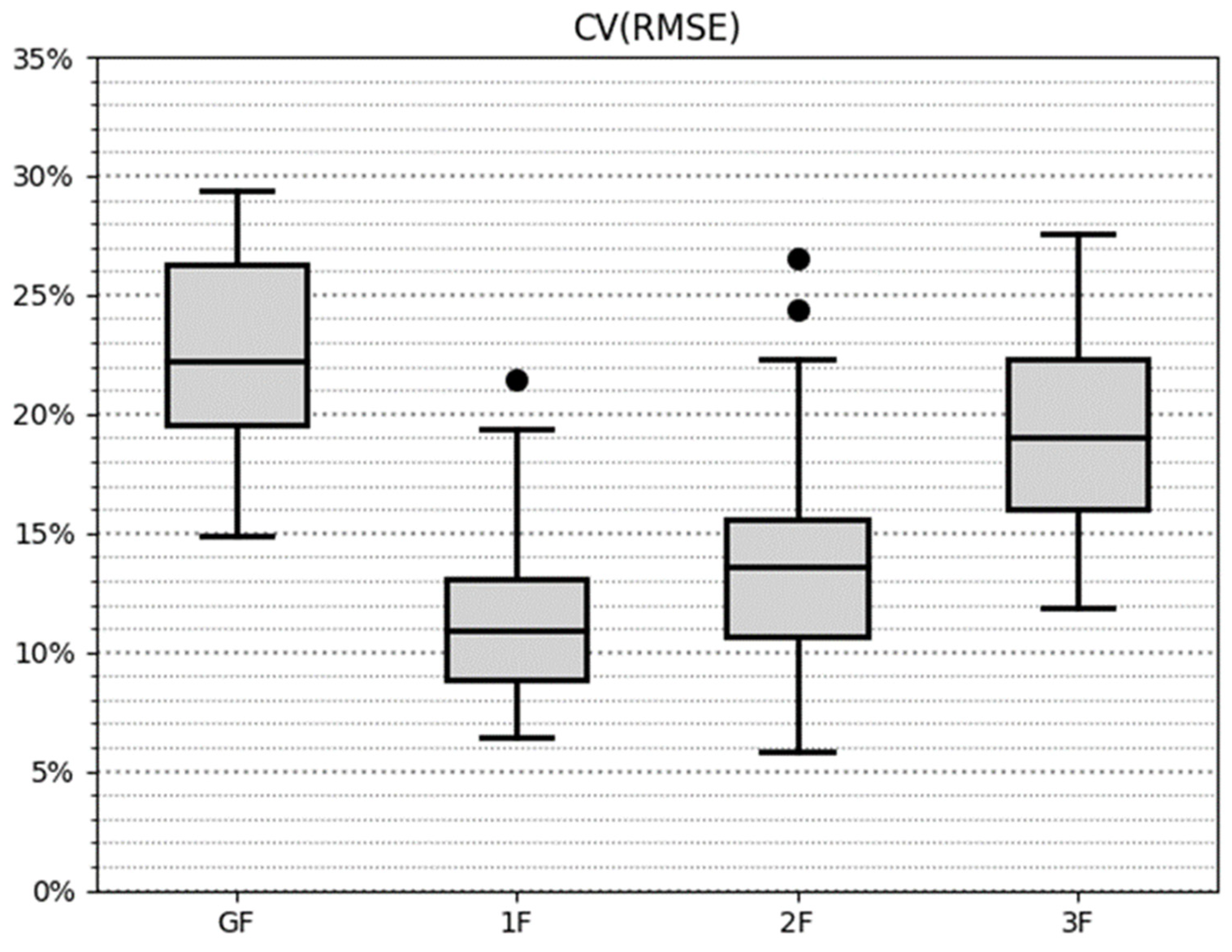
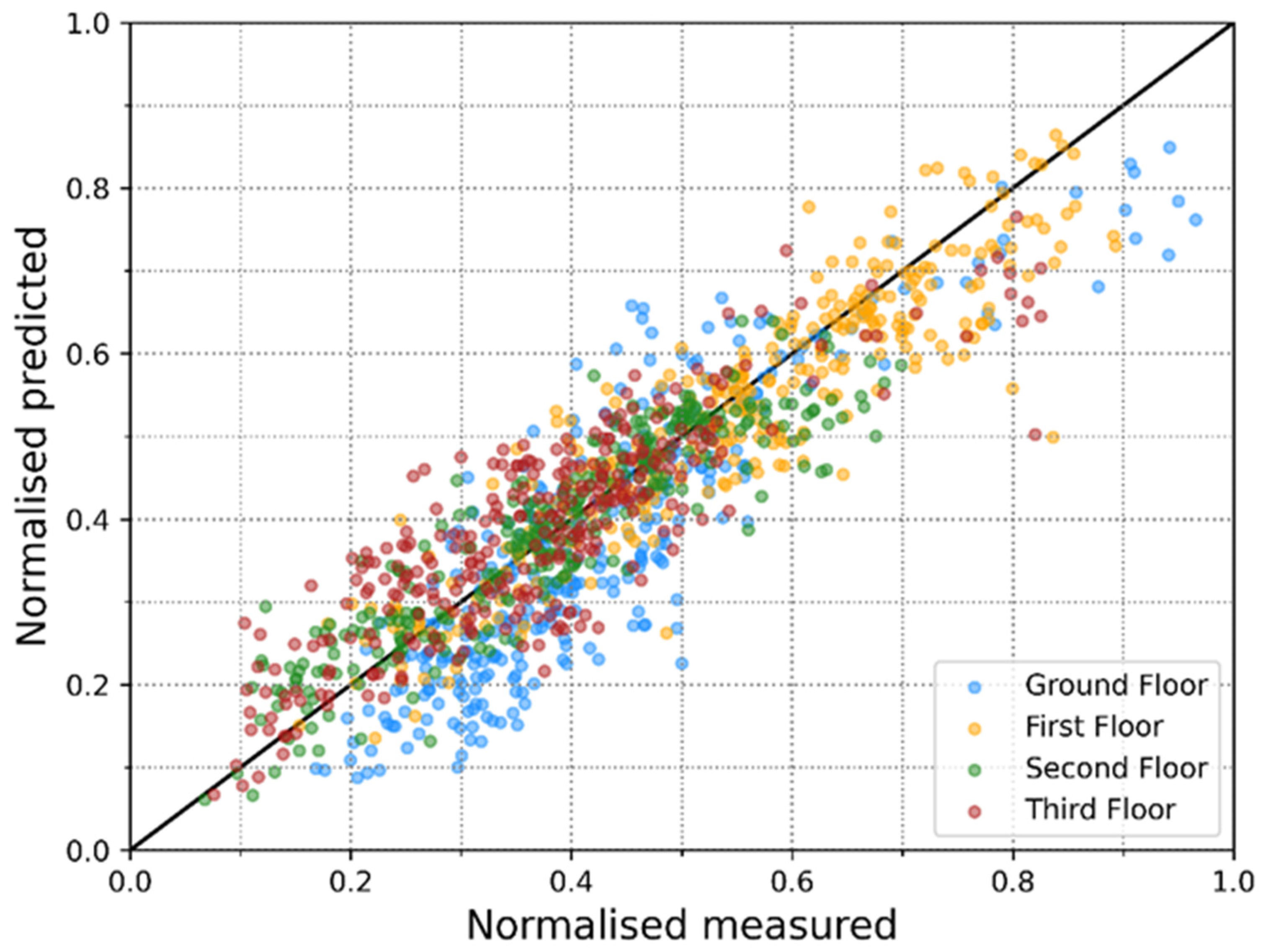
4.2. Error Measurement and Performance Analysis

The prediction sample covered four working weeks. Forecasting techniques were applied to the entire period but only working hours were taken into account in the calculation of the error, due to the need of LSTM networks to work with continuous periods of time and the fact that error calculation using constant values of zero does not provide actual information on the accuracy of the model. For each floor, the average temperature was maintained around 21.7 °C, except for the 3F, where it reached 23.8 °C.

To avoid plotting large series, a comparison of CV(RMSE) by week was done between each of the four complete weeks and the monthly value. The selected week for every floor plot was the one with the closest CV(RMSE) to the mean value. Figure 5 illustrates the result of applying this criterion.

The results show that LSTM models were capable of replicating the trend of the thermal demand of the building. The model catches the initial peak of each day with high accuracy, especially on the 1F and 2F. The main characteristic that distinguishes these floors from the two others is that they are not so influenced by a source of heat or cold, which happens on the 3F with solar radiation or on the GF with the influence of air currents caused by the racking of people in the building.

This has a consequence that the GF has the greatest difference between the initial peak and the rear damping, with a difference of almost 20 kW. Graphics for the rest of the floors have almost the same shape, with some exception for the 1F and 2F where the heat demand grows during all the working hours.

As mentioned in Section 4.1, the 3F is more sensitive to weather changes, due to having the largest surface in contact with the exterior. Observing the high thermal demand in the initial peak, which is greater than for the 1F, it can be deduced that the heat losses during the night are greater for this floor.

CV(RMSE) and MBE results are summarized in

Table 3. Monthly calculation (Mean) and Standard Deviation (SD) of CV(RMSE) and MBE errors for heat demand prediction for each floor.

	CV(RMSE) [%]		MBE
Floor	Mean	SD	Mean	SD
GF	21.12	4.33	11.92	4.79
1F	12.71	4.13	3.65	5.21
2F	15.92	5.38	−1.04	8.81
3F	19.50	4.52	−5.01	11.96

, including the value for the entire working days prediction series and the Standard Deviation from it.

The error results included in Table 3 are consistent with the graphics. The GF has the biggest CV(RMSE) and a positive MBE higher than the rest of the floors, which means that the model is producing an underestimation. For the CV the results maintain a Standard Deviation very similar on each floor. Conversely, results for MBE show a very different dispersion for each floor. The GF and the 1F present a low dispersion, with a SD close to 5, while for the 2F and the 3F are close to 10%, below and above, respectively. These two floors have a MBE < 0, which means an overestimation. As can be seen, the MBE value for the 2F is very close to 0 but with a high dispersion, which means an equilibrium around the mean. On the contrary, the 3F shows a clear tendency to overestimation, with a negative MBE and a high Standard Deviation. It is also worth mentioning the effect the horizontal distribution of each plant has on the error. The GF, having the sensors installed in three rooms of low surface, means its profile is more sensitive to the accumulation of heat, while the first and third, being composed of larger rooms, reduce the influence of said accumulation.

To illustrate CV(RMSE) per floor Figure 6 was extracted. This figure was obtained applying the CV(RMSE) formula to each day. Instead of using daily mean value, the mean value of the entire series was used to obtain comparable magnitudes. As shown on the figure, median value and the CV(RMSE) of each floor are practically coincident.

The 1F and 2F have narrower boxes, but at the same time they have proportionally wider whiskers and atypical values. Both also show the smallest error CV(RMSE) values while the GF and 3F present a broader and bigger quartile range but do not have outlier values. For all floors, boxes have a size between 4% and 6.5%, which is synonymous with good stability of the results.

On the other hand, to explain the MBE results of the predictions in the different thermal demand segments, the results have been adimensionalized using the maximum allowable thermal demand, 35 kW, and plotted facing the measured value with the forecasting value. The four floors are plotted together using this method in Figure 7.

The graph shows how thermal demand is generally below 70% of the maximum capacity of the installation for all floors. Analysing in detail each floor, as seen in Figure 5, the GF produces an underestimation of the highest and the lowest values, maintaining a good accuracy of medium values. The 1F has a low dispersion with a few atypical values, but generally remains closer to the mean value than the rest of the floors.

The 2F has the lowest heat demand, probably influenced by its placement between two floors which means an energy contribution through horizontal enclosures. This graph also shows the behavior explained previously, reflected on the 2F with a stacking of dots around the mean. For the 3F, the overestimation is appreciable observing how the dots are placed straight above the x = y.

4.3. HLC Comparison

HLC simple is obtained for a total of three periods. Two of them have been previously obtained by Uriarte et al. [23] and will be used to evaluate the accuracy of our model. Sample 1 comprises from 17 January 2018 4:00 to 20 January 2018 6:00 and Sample 2 includes from 6 February 2018 17:00 to 10 February 2018 7:00. Subsequently, a period that meets the specifications indicated in Section 2.2 has been sought to extrapolate the applied methodology. To obtain this period, solar radiation gains have been calculated using solar radiation and the horizontal surface of the west block, 158.6 m², provided by Erkoreka et al. [25]. The thermal conditions of these three periods are summarized in

Table 4. Thermal conditions for the three periods analyzed. All variables are averaged for the period.

Period	T_In-T_Out [K]	Q [kW]	Q + K [kW]	Rad/(Q + K) [%]
Sample 1	14.98	33.72	49.53	9.73%
Sample 2	19.68	42.12	56.64	5.70%
Sample 3	17.70	26.55	41.54	9.79%

.

The conditions for the samples are very similar. The Sample 3, in comparison with Sample 1 has a bigger temperature difference but a smaller heat demand, due to higher solar heat gains. The same sample compared to Sample 2 shows a smaller magnitude on every variable. The results for the HLC simple calculation on the periods are recorded on

Table 5. HLC simple obtained per floor and for the entire building.

Period	GF [kW/K]	1F [kW/K]	2F [kW/K]	3F [kW/K]	Building (Predicted) [kW/K]	Building (Real) [kW/K]
Sample 1	0.61	1.01	0.71	0.80	3.13	3.27
Sample 2	0.56	0.87	0.67	0.71	2.81	2.85
Sample 3	0.46	0.79	0.55	0.64	2.44	2.35

.

For the HLC calculated on each floor, the difference between the obtained value using monitored data and using forecasting techniques moves in the interval ±0.03.

From these results, it can be deduced that in days with a higher temperature difference the obtained HLC simple for the predicted values is closer to the real HLC simple. This is because the days with a greater temperature difference present a higher thermal demand. As a consequence, the terms of occupation and the solar gains are of lesser importance, which are the factors that add variability. The opposite effect can be seen in the results of Samples 1 and 3, where the Rad/Q + K ratio is higher.

Based on the results per plant, it should be noted that the GF is the one that contributes the least to HLC, with the 1F being the one that has the greatest importance in obtaining this coefficient. This result is in line with the fact that the 1F has the highest thermal demand but also the highest contribution for occupation thermal loads.

5. Conclusions

This paper presents a new use of LSTM neural networks for thermal demands forecasting on buildings, giving relevance to the accurate detection of the thermal inertia. At the same time, it also demonstrates that it is feasible to estimate the HLC with great precision using these forecasting techniques. The study was conducted by analysing monitored data of the Rectorate building of UPV/EHU. In the study, the variables monitored in the Rectorate building of UPV/EHU have been used, among which are included the interior conditions, the exterior environmental conditions and the information provided by the heating and electrical installation.

The results obtained show that LSTM neural networks models are capable of estimating the thermal demands of in-use buildings with a CV(RMSE) of 21% for the worst case and 12% for the best. These errors show that black-box models based on LSTM neural networks produce errors below the condition established by ASHRAE to consider a model calibrated. To achieve those results, the detection of the appropriate time-lag for the building for a correct treatment of the building under study is necessary.

The thermal demand values obtained by the created model are used to estimate the HLC value. In this case, the error does not exceed 4%, which proves that the methodology is valid to estimate this coefficient without the need to keep the building’s thermal conditions controlled so that they are considered stationary.

The main contribution of this paper is the development of a methodology for the detection of thermal inertia, the prediction of thermal demands and the estimation of the HLC that can be applicable to other types of buildings. The variables used in this paper are commonly monitored in different types of buildings, and weather variables are readily available. Therefore, the methodology described here can be extrapolated to different buildings, such as residential, industrial, or educational, to assess their energy and thermal performance.

On one hand, the limitations of this methodology are through the difficulties of obtaining the conditions to calculate the HLC, which can restrict the obtained conditions to short periods where the solar radiation gains are very small or the heat demand very high, so that the relative solar influence is low. On the other hand, buildings without a precise source of weather data may open a future work line to combine the methodology described with meteorological data collection techniques to avoid expensive outdoor monitoring systems.

References

1. Project, O.-M. Energy Efficiency Trends and Policies in the Household and Tertiary Sectors. 2015. Available online: https://www.odyssee-mure.eu/publications/archives/energy-efficiency-trends-policies-buildings.pdf (accessed on 17 August 2021).
2. Directorate-General for Research and Innovation. 100 Climate-Neutral Cities by 2030—By and for the Citizens Publications Office of the EU; European Commission: Luxenburg, 2020. [Google Scholar]
3. Zou, P.X.; Wagle, D.; Alam, M. Strategies for minimizing building energy performance gaps between the design intend and the reality. Energy Build. 2019, 191, 31–41. [Google Scholar] [CrossRef]
4. Menezes, A.C.; Cripps, A.; Bouchlaghem, D.; Buswell, R. Predicted vs. actual energy performance of non-domestic buildings: Using post-occupancy evaluation data to reduce the performance gap. Appl. Energy 2012, 97, 355–364. [Google Scholar] [CrossRef] [Green Version]
5. van Dronkelaar, C.; Dowson, M.; Spataru, C.; Mumovic, D. A Review of the Regulatory Energy Performance Gap and Its Underlying Causes in Non-domestic Buildings. Front. Mech. Eng. 2016, 1. [Google Scholar] [CrossRef] [Green Version]
6. Kim, Y.; Bande, L.; Aoul, K.; Altan, H. Dynamic Energy Performance Gap Analysis of a University Building: Case Studies at UAE University Campus, UAE. Sustainability 2020, 13, 120. [Google Scholar] [CrossRef]
7. Li, X.; Wen, J. Building energy consumption on-line forecasting using physics based system identification. Energy Build. 2014, 82, 1–12. [Google Scholar] [CrossRef]
8. Martínez, S.; Eguía, P.; Granada, E.; Moazami, A.; Hamdy, M. A performance comparison of multi-objective optimization-based approaches for calibrating white-box building energy models. Energy Build. 2020, 216, 109942. [Google Scholar] [CrossRef]
9. Narayanan, M.; De Lima, A.; Dantas, A.D.A.; Commerell, W. Development of a Coupled TRNSYS-MATLAB Simulation Framework for Model Predictive Control of Integrated Electrical and Thermal Residential Renewable Energy System. Energies 2020, 13, 5761. [Google Scholar] [CrossRef]
10. Figueiredo, A.; Kämpf, J.; Vicente, R.; Oliveira, R.; Silva, T. Comparison between monitored and simulated data using evolutionary algorithms: Reducing the performance gap in dynamic building simulation. J. Build. Eng. 2018, 17, 96–106. [Google Scholar] [CrossRef]
11. Martínez-Mariño, S.; Eguía-Oller, P.; Granada-Álvarez, E.; Erkoreka-González, A. Simulation and validation of indoor temperatures and relative humidity in multi-zone buildings under occupancy conditions using multi-objective calibration. Build. Environ. 2021, 200, 107973. [Google Scholar] [CrossRef]
12. Balboa-Fernández, M.; De Simón-Martín, M.; González-Martínez, A.; Rosales-Asensio, E. Analysis of District Heating and Cooling systems in Spain. Energy Rep. 2020, 6, 532–537. [Google Scholar] [CrossRef]
13. Xue, G.; Pan, Y.; Lin, T.; Song, J.; Qi, C.; Wang, Z. District Heating Load Prediction Algorithm Based on Feature Fusion LSTM Model. Energies 2019, 12, 2122. [Google Scholar] [CrossRef] [Green Version]
14. Song, J.; Zhang, L.; Xue, G.; Ma, Y.; Gao, S.; Jiang, Q. Predicting hourly heating load in a district heating system based on a hybrid CNN-LSTM model. Energy Build. 2021, 243, 110998. [Google Scholar] [CrossRef]
15. Helm, J.M.; Swiergosz, A.M.; Haeberle, H.; Karnuta, J.M.; Schaffer, J.L.; Krebs, V.E.; Spitzer, A.I.; Ramkumar, P.N. Machine Learning and Artificial Intelligence: Definitions, Applications, and Future Directions. Curr. Rev. Musculoskelet. Med. 2020, 13, 69–76. [Google Scholar] [CrossRef]
16. Comesaña, M.M.; Febrero-Garrido, L.; Troncoso-Pastoriza, F.; Martínez-Torres, J. Prediction of Building’s Thermal Performance Using LSTM and MLP Neural Networks. Appl. Sci. 2020, 10, 7439. [Google Scholar] [CrossRef]
17. Li, Z.; Friedrich, D.; Harrison, G.P. Demand Forecasting for a Mixed-Use Building Using Agent-Schedule Information with a Data-Driven Model. Energies 2020, 13, 780. [Google Scholar] [CrossRef] [Green Version]
18. Franchina, L.; Sergiani, F. High Quality Dataset for Machine Learning in the Business Intelligence Domain. In Proceedings of the SAI Intelligent Systems Conference, London, UK, 5–6 September 2019; Springer: Cham, Switzerland, 2019. [Google Scholar]
19. Wan, L.; Sun, D.; Deng, J. Application of IOT in building energy consumption supervision. In Proceedings of the 2010 International Conference on Anti-Counterfeiting, Security and Identification, Chengdu, China, 18–20 July 2010; pp. 169–172. [Google Scholar]
20. Chaouch, H.; Çeken, C.; Arı, S. Energy management of HVAC Systems in smart buildings by using fuzzy logic and M2M communication. J. Build. Eng. 2021, 44, 102606. [Google Scholar] [CrossRef]
21. Hochreiter, S.; Schmidhuber, J. Long Short-Term Memory. Neural Comput. 1997, 9, 1735–1780. [Google Scholar] [CrossRef]
22. ASHRAE. Guideline 14-2014—Measurement of Energy, Demand, and Water Savings; ASHRAE: Atlanta, GA, USA, 2014. [Google Scholar]
23. Uriarte, I.; Erkoreka, A.; Soto, C.G.; Martin, K.; Uriarte, A.; Eguia, P. Mathematical development of an average method for estimating the reduction of the Heat Loss Coefficient of an energetically retrofitted occupied office building. Energy Build. 2019, 192, 101–122. [Google Scholar] [CrossRef]
24. Comesaña, M.M.; Mariño, S.M.; Eguía-Oller, P.; Granada-Álvarez, E.; González, A.E.; Erkoreka, A.A. A Functional Data Analysis for Assessing the Impact of a Retrofitting in the Energy Performance of a Building. Mathematics 2020, 8, 547. [Google Scholar] [CrossRef] [Green Version]
25. Erkoreka, A.; Garcia, E.; Martin, K.; Teres-Zubiaga, J.; Del Portillo, L. In-use office building energy characterization through basic monitoring and modelling. Energy Build. 2016, 119, 256–266. [Google Scholar] [CrossRef]
26. Eckle, K.; Schmidt-Hieber, J. A comparison of deep networks with ReLU activation function and linear spline-type methods. Neural Netw. 2018, 110, 232–242. [Google Scholar] [CrossRef] [PubMed]
27. Bock, S.; Weis, M. A Proof of Local Convergence for the Adam Optimizer. In Proceedings of the 2019 International Joint Conference on Neural Networks, IJCNN 2019, Budapest, Hungary, 14–19 July 2019; pp. 1–8. [Google Scholar]
28. Li, M.; Zhang, T.; Chen, Y.; Smola, A.J. Efficient mini-batch training for stochastic optimization. In Proceedings of the 20th ACM SIGKDD International Conference on Knowledge Discovery and Data Mining, KDD 2014, New York, NY, USA, 24 August 2014; pp. 661–670. [Google Scholar]
Figure 1. LSTM cell internal structure.
Energies 14 05188 g001
Figure 2. Rectorate building of the UPV/EHU located on Leioa, Vizcaya, in the north of Spain. (a) Plan view of the building of the blocks: 1-west block; 2-central block; 3-east block. (b) Façade view of the west block.
Energies 14 05188 g002
Figure 3. Sensor distribution on each floor. Temperature, humidity, and CO2 sensors are marked as green squares, while blue and red squares indicate the electric consumption and thermal demand sensors, respectively. (a) Ground Floor, (b) First Floor, (c) Second Floor, (d) Third Floor.
Energies 14 05188 g003aEnergies 14 05188 g003b
Figure 4. Input dataset classification.
Energies 14 05188 g004
Figure 5. Results of thermal demand predictions on GF (top left), 1F (top right), 2F (bottom left) and 3F (bottom right).
Energies 14 05188 g005
Figure 6. Boxplot of the CV(RMSE) results for every floor.
Energies 14 05188 g006
Figure 7. Normalized dispersion of the results.
Energies 14 05188 g007