Measurement and Simulation of Flow in a Section of a Mine Gallery

Abstract

Research work on the air flow in mine workings frequently utilises computer techniques in the form of numeric simulations. However, it is very often necessary to apply simplifications when building a geometrical model. The assumption of constant model geometry on its entire length is one of the most frequent simplifications. This results in a substantial shortening of the geometrical model building process, and a concomitant shortening of the time of numerical computations; however, it is not known to what extent such simplifications worsen the accuracy of simulation results. The paper presents a new methodology that enables precise reproduction of the studied mine gallery and the obtaining of a satisfactory match between simulation results and in-situ measurements. It utilises the processing of data from laser scanning of a mine gallery, simultaneous multi-point measurements of the velocity field at selected gallery cross-sections, unique for mine conditions, and the SAS turbulence model, recently introduced to engineering analyses of flow issues.

1. Introduction

Proper operation of mine ventilation is one of the necessary conditions for the safe and effective functioning of underground mines. Ventilation systems ensure such a condition of atmosphere that enables normal mine operations, and also prevent or possibly minimise the effects of failures and disasters, if any. For many years, mine ventilation used methods of computational fluid dynamics, which were developed for other fields, such as aviation, construction of fluid-flow machines, the automotive industry and meteorology. In particular, it was related to applications of the finite volume method to resolve equations of fluid mechanics [1]. In each of the aforementioned fields, and even individual issues, to achieve a satisfactory quality of numerical modelling, it was necessary to find or develop a specific methodology and to verify it experimentally. An example of the methodology for solving particular problems such as the effect of machine-mounted dust scrubbers on the performance of face ventilation systems can be found in [2]. Other applications of CFD have been described by Ren and Balusu in [3]. An updated review of CFD applications in mining can be found in [4]. More recent work refers to similar supports, but in roadways of rectangular shape [5] Despite the above-mentioned solutions, for many cases, the issues of numerical modelling of flow effects in mines encounter numerous problems, which so far have not been resolved to a satisfactory degree. They result inter alia from the vastness of such ventilation systems, frequently comprising hundreds of kilometers of workings with complicated and irregular shapes. Such irregularities result from, for example, difficult to predict local deformations caused by the pressure of surrounding strata. Previous measuring techniques did not provide a practical possibility to take such irregularities into consideration.

The non-stationary nature of a flow is another issue. An irregular shape of the workings and the presence of numerous objects that are significant for the operation of a mine, which must fit into the limited space of underground workings, causes substantial local flow disturbances. This results in difficulties in achieving satisfactory mapping of the flow by means of previous generation turbulence models [6]. Furthermore, so far, there has been a very small number of papers addressing specific flow conditions in galleries with the arched roof support.

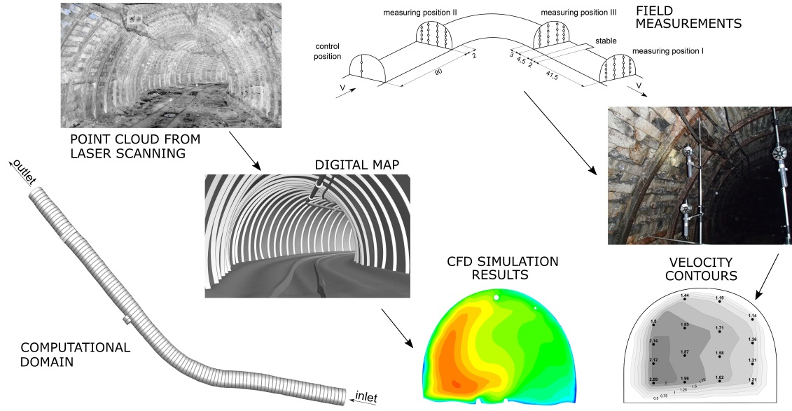
Mines frequently operate under conditions of coexisting hazards and feature difficult environmental conditions [7]. This results in particular difficulties when acquiring experimental data, necessary for verification and validation of modelling. This paper presents the application of novel measuring and numerical modelling techniques, which allow one to achieve a satisfactory match between simulation results and measurement data. They were applied to a section of a gallery with a shape and environmental conditions representative of Polish coal mines. The obtained results are a point of reference for further analyses of the influence of geometry representation simplifications on the accuracy of numerical simulations. This work aims at the optimisation of numerical modelling in order to achieve sufficient reliability whilst minimising the computation time and the level of power involved.

Accurate reproduction of the geometry of the gallery was obtained by means of terrestrial laser scanning [8,9,10]. The computation area geometry was determined based on this. This method has so far been applied for the CFD modeling of problems that are remote from mine ventilation, such as the flows around Formula I cars or around the human body. The results of recent work [11] show application to much closer problems. This paper both confirms the methodology used and presents solutions that can reduce the workload involved in transferring the scaning data into meshable geometry.

The data on the velocity field were obtained by means of a system of simultaneous multi-point measurements of flow velocity using intrinsically safe vane anemometers, developed with the authors’ contribution.

A sequence of flow simulations, using several turbulence models from the classical k-e, through k-wSST, to the recently introduced Scale Adaptive Simulation method, has been performed in search of the best method. The latter, described in [12] has turned out to provide remarkably better fit to the experimental data then the alternative.

2. Description of the Object of Studies and of the Method for Computation Area Geometry Determination

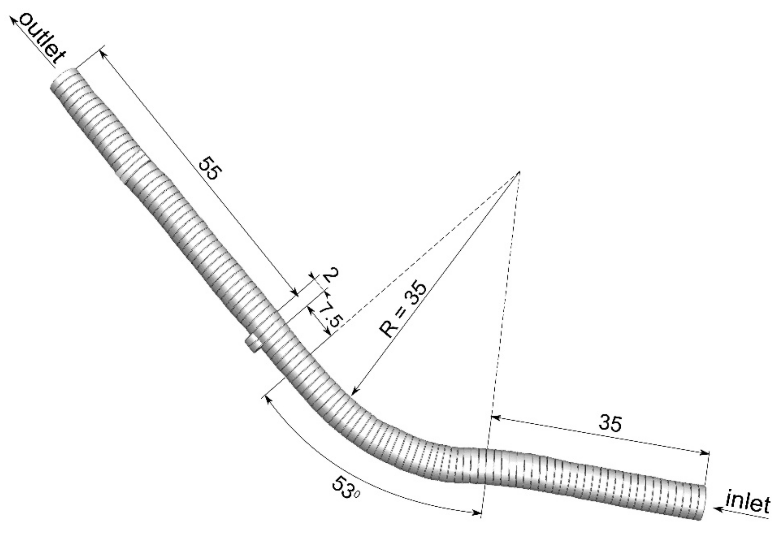
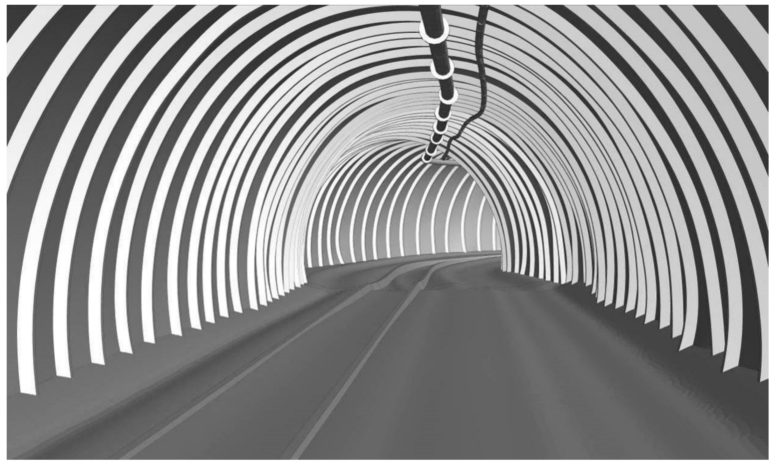
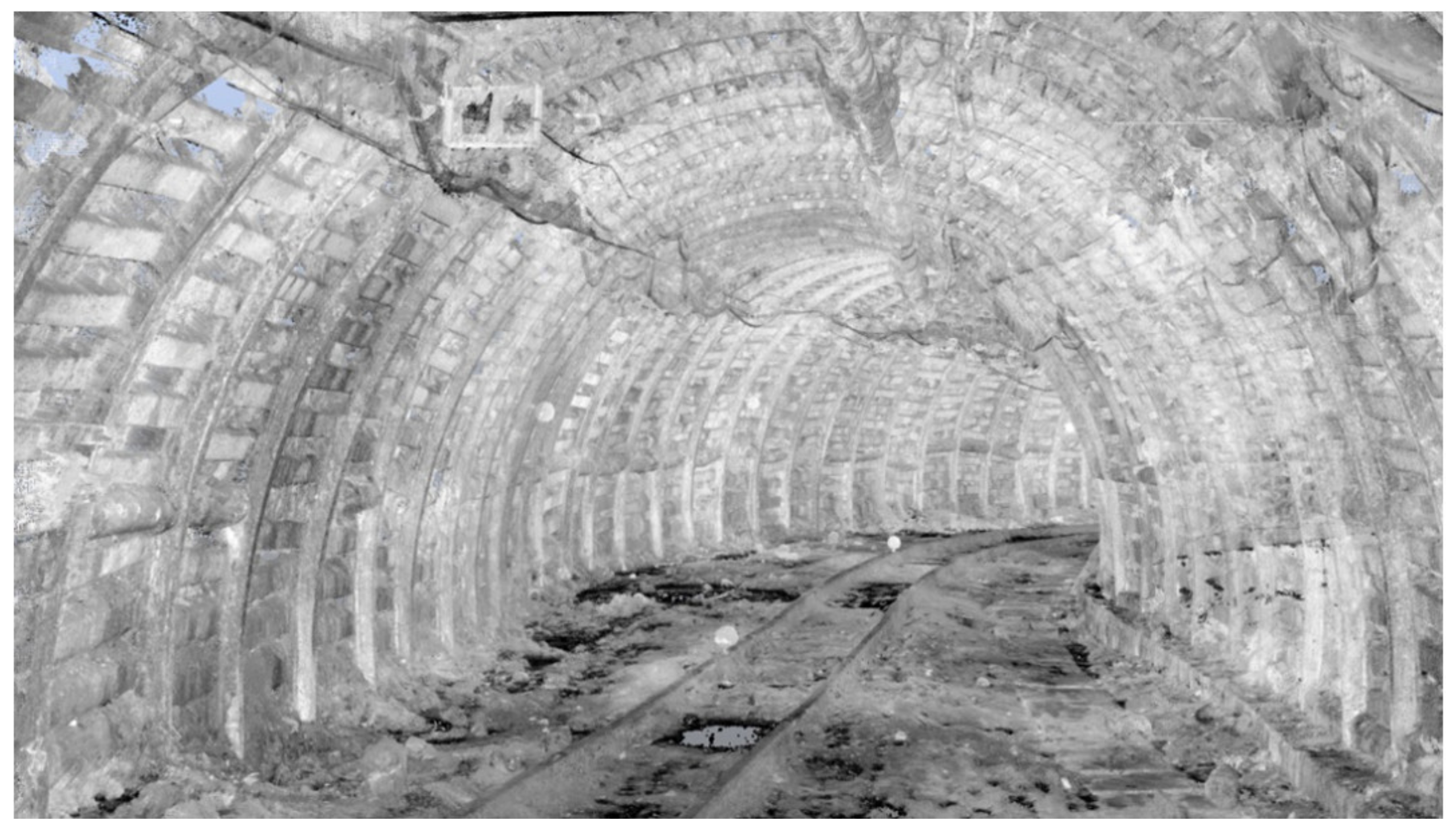
A fragment of the Grodzisko crosscut located at the Sobieski coal mine was selected. It consisted of two apparently straight sections connected with a bend (see Figure 1). The total length of the analysed section was 132 m. The section was almost horizontal. The floor was covered with mildly waved mud and some water pools. The gallery had an arched support with an initial cross-section of 13 m². It was formed several years ago, and the pressure of the surrounding rocks introduced irregular deformations of the initial shape [13], resulting in approx. 12% variability of the cross-sectional area (see Figure 2). The gallery was free from obstacles except for two pipelines and rails on the floor. This object can be considered as being representative of Polish collieries, and its location allowed for several hours of measurement sessions without interfering with production activities.

2.1. Determination of the Object Geometry by Means of the Laser Scanning Technique

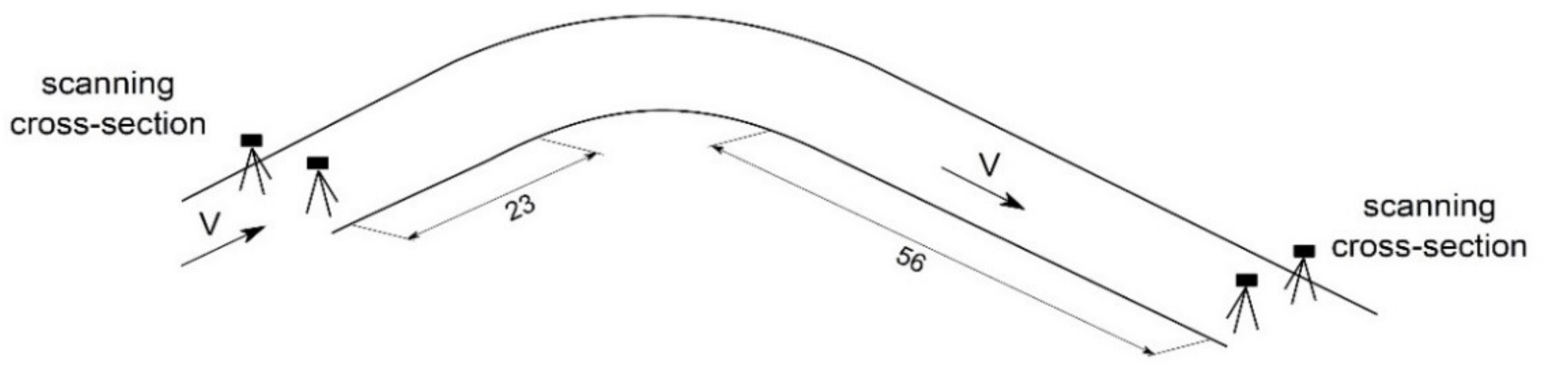
To obtain a complete spatial model of the workings, the entire section of gallery was divided into 11 scanning cross-sections, which provided 22 measuring positions. The first scanning cross-section was set approx. 23.0 m before the inlet to the bend, while the last scanning section was approx. 56.0 m behind the outlet from the bend (Figure 3).

The processing of sets acquired by the laser scanner can be referred to as pre-processing. The measurement data processing required preparation of the data for further processing. At this stage, the most important processes should include the orientation of a point cloud through the combination of a few point clouds (obtained from individual measuring positions) into one data set [9]. The point cloud was then filtered, which consisted in cleaning and removing measurement noise and discontinuities [14]. The laser scanning of the Grodzisko crosscut geometry, the obtained point cloud pre-processing and the reduction in the number of points resulted in the obtaining of a very good digital reproduction of the entire space of the scanned gallery fragment, consisting of 152 million points (Figure 2) [8].

This cloud, however, was far too complex to be directly used by available comoutational mesh generation software. For computational mesh generation, it is recommended to simplify the geometry, neglecting details unnecessary for the flow simulation. Further simplification of boundary geometry could not be conducted automatically without losing important details such as ribs. Therefore, the shape of working had to be manually redrawn using the point cloud as a template. As a result, the geometry of the geometrical model was obtained with accurate reproduction of the actual object shape (Figure 4).

The computation area, comprising 110 arches of ŁP support, a hydraulic pipe, a pipeline and rails of a mine railway, consisted of (Figure 1):

• Straight section before the bend, 35 m long;
• Section of the bend, with a turning radius of 35 m, and an angle of rotation of 53°;
• Straight section behind the bend, 64.5 m long, taking into account the existence of a stable, 2.0 m long at a distance of 7.5 m behind the outlet from the bend.

2.2. Generation of the Numerical Grid

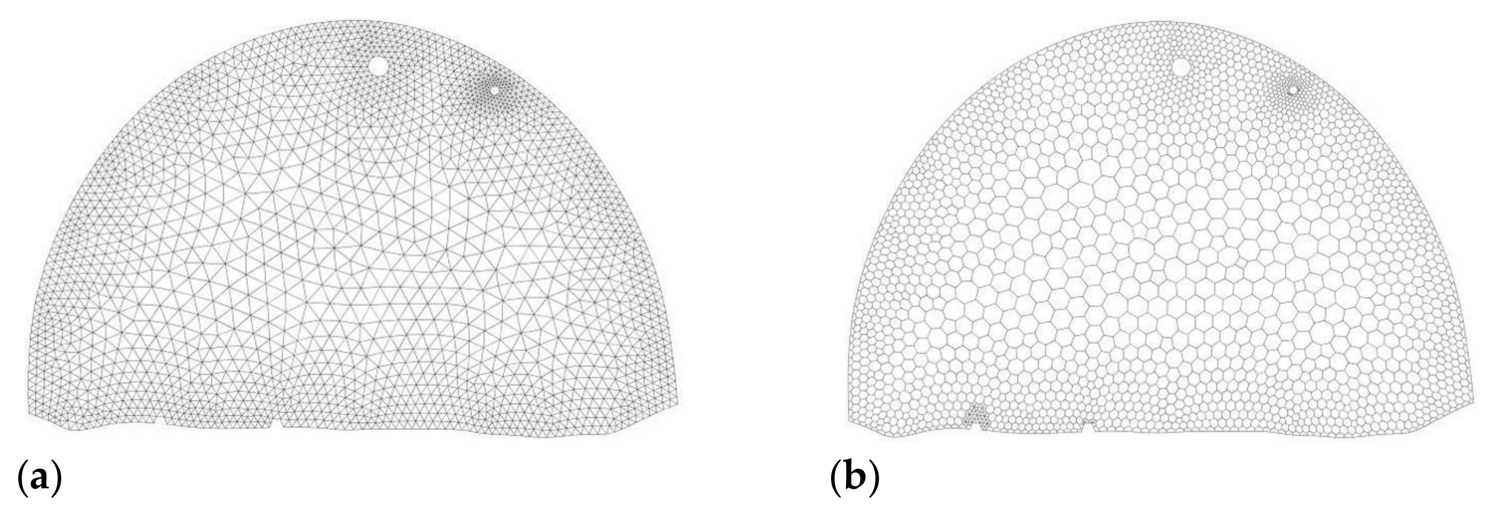
Application of the finite volume method required division of the computational domain into a set of interconnected volumes, which is referred to as generation of the numerical grid. The geometries of the area and the arrangement of flow directions, which are difficult to predict, in the entire numerical model justified application of tetrahedral or polyhedral volumes of a uniform size in every direction. The grid density increased towards the boundaries due to application of the size function, which allowed for control of the computational grid size close to a selected point, edge or surface. Numerical models were initially meshed with tetrahedral non-structural grids, which were then converted to a polyhedral grid (Figure 5). Thanks to the conversion, the number of cells decreased, which significantly shortened the time of the numerical calculations.

A dimensionless parameter of length y⁺ for the computational area falls within a range of 10 ≤ y⁺ ≤ 440. The number of cells within a range of 10 ≤ y⁺ ≤ 30 is small, which allows for acceptance of the grid quality in terms of a dimensionless parameter of length y⁺.

The skewness factor for the numerical grid, with the parameters also presented, is shown in

Table 1. Percentage share of numerical grid cells for skewness factor ranges.

Skewness Factor	Percentage Share (%)	Cell Quality
1	0.00	degenerate
0.9 < 1	0.00	bad
0.75–0.9	0.00	poor
0.5–0.75	10.17	fair
0.2–0.5	52.37	good
0 > 0.25	29.24	excellent
0	8.22	equilateral

in the form of a percentage share of grid cells in a specific range of skewness factor.

3. Measurements of the Air Velocity Profile in the Mine Workings

In situ measurements provided data for setting the flow boundary conditions and verification of simulation results. For this purpose, three cross-sections of the gallery were selected. Specific mine conditions allowed for the application of an in-house designed and manufactured the Multipoint System of Flow Velocity Measurements (known as the SWPPP system) [15].

Multipoint measurements have been carried out by several researchers; for example, simultaneous methane concentration sampling by Wala et al. [2] or sequential velocity measurements by Martikainen et al. [16]. In most cases, however, this measurement was sequential, conducted with a single instrument repositioned from one point to another. This method provides proper information on the velocity field if the flow is sufficiently steady and the point averaging periods are sufficiently long. Simultaneous measurement eliminates this source of uncertainty and enables the obtaining of the data in a shorter time.

Measurements with the use of the SWPPP system consist of placing the appropriate number of vane anemometers in the mine drift cross-section and then simultaneously measuring the air flow velocity. To calculate the volumetric flow rate, the cross section of a mine drift, where the measurement takes places, needs to be integrated. In reality, it is impossible to measure the whole velocity field in cross-section. That is why the flow velocity is measured in a finite number of points on this surface and then, based on the results, the velocity distribution is estimated using the linear triangulation. This method consists of dividing the cross-section area into triangular areas so that the vertices of the triangles are points at which the flow velocity is known from the measurements.

To place the anemometric sensors in the selected cross-section points of the gallery, it was necessary to use an appropriate bearing structure consisting of four vertical beams, to which the anemometers were fixed, and one or two horizontal stiffening beams. The vane anemometers were fixed on vertical beams. The number of sensors could be adapted to the working’s cross-section, with this being a compromise between ensuring the required precision of distribution determination and achieving the smallest possible interference into the flow itself.

The properties of the velocity sensors are listed below:

• Measuring range of flow velocities: ±(0.2–20 m/s);
• Measuring error of flow velocities: ±(0.5% rdg + 0.02 m/s);
• Measurement resolution: 0.01 m/s;
• Frequency of measurements: 1 Hz.

Before measurements, each of the 18 methane anemometers used in the SWPPP system [17] were adjusted in the aerodynamic tunnel of the Calibration Laboratory for Ventilation Measuring Instruments of the IMG-PAN, which has received accreditation from the Polish Centre for Accreditation.

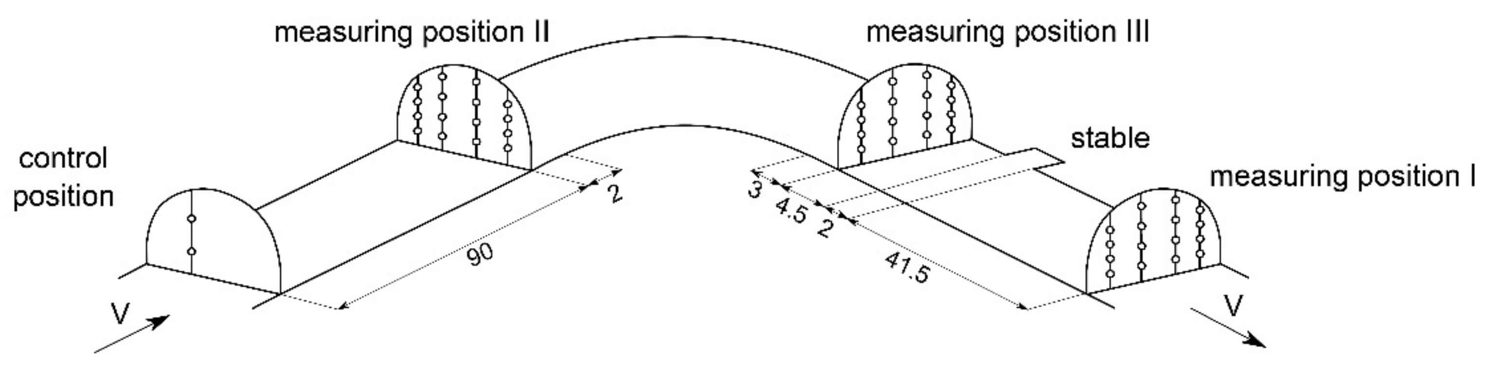
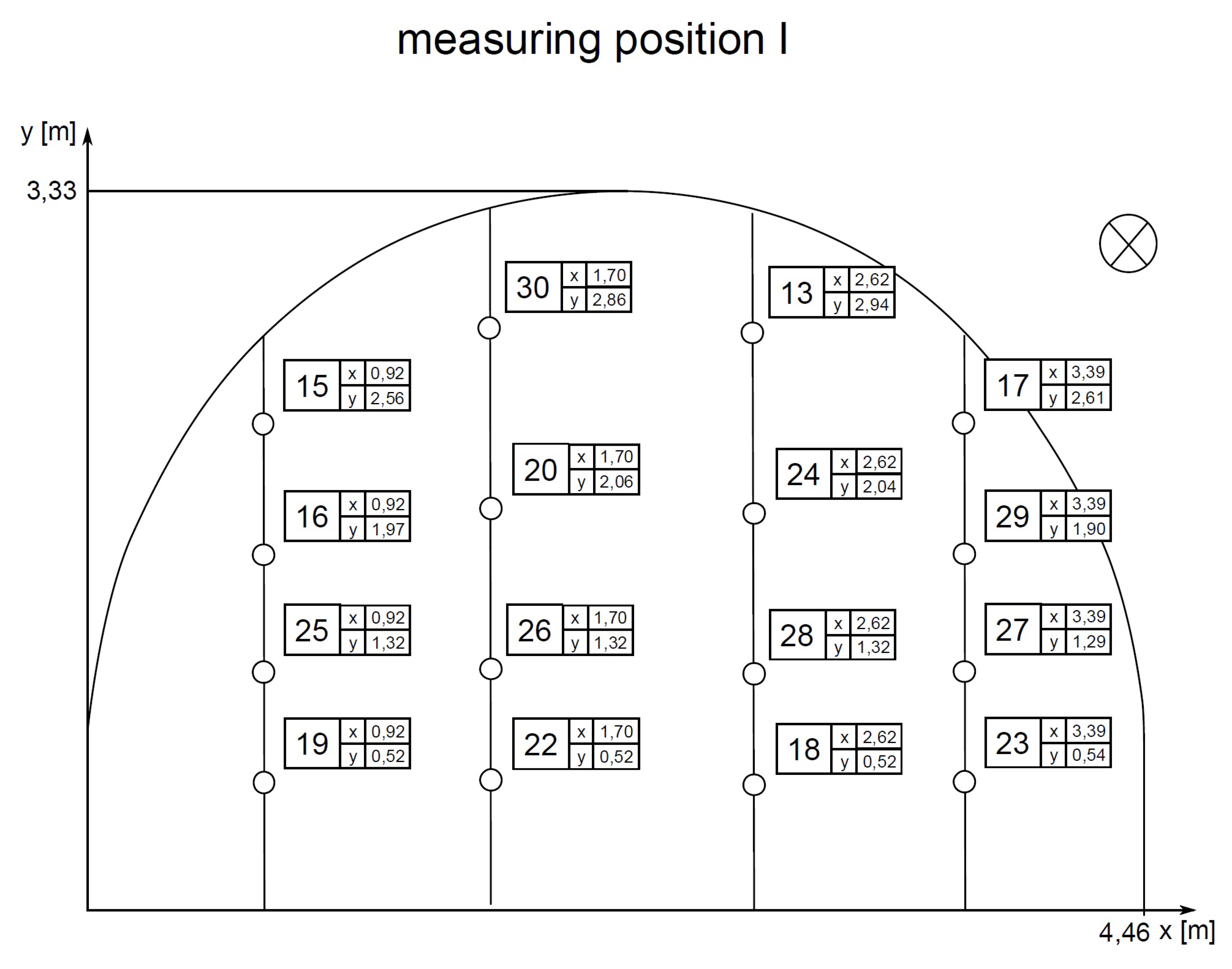
Measurements by means of the SWPPP system were performed at three measuring cross-sections, presented in Figure 6. After recording flow conditions at Position I, the set of 16 anemometers was moved to Position II and then to Position III. Simultaneously, laser scanning was performed in such a manner as to exclude interference with the flow measurements. Cross-section II was to provide the initial boundary conditions, and Positions III and I were used for verification. Vane anemometers measure the velocity component parallel to their axis; therefore, all positions were in places where a dominant velocity component parallel to the gallery axis may be expected.

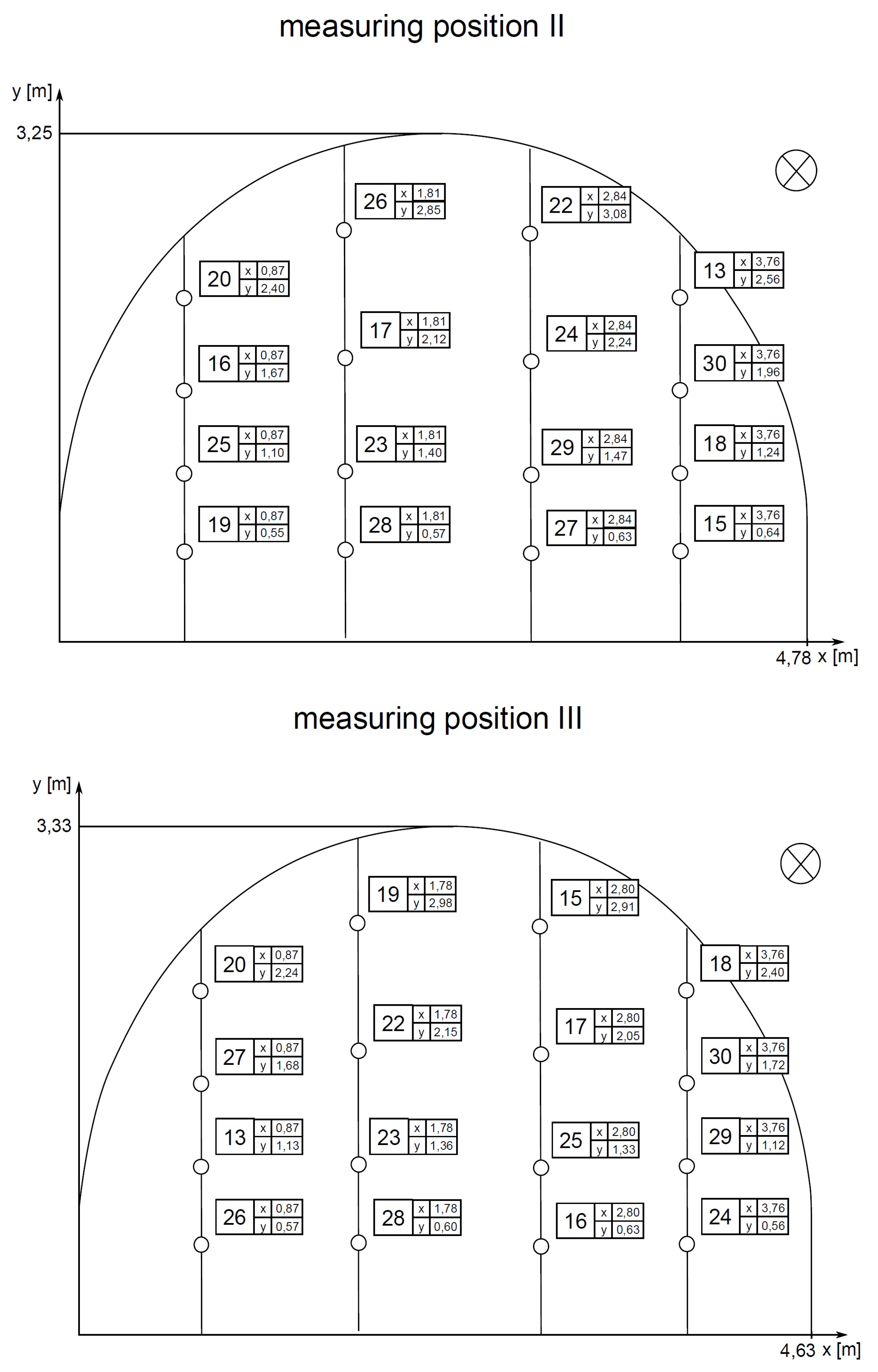
The arrangement of measuring points in the cross-sections of measuring positions, together with their coordinates, is presented in Figure 7. In addition, each measuring point was marked with a number corresponding to the anemometer number.

Two anemometers on a vertical line, 90 m before Position II, continuously recorded velocity to detect variations of the flow rate, if any. Their readings were used to trim the results from Positions I to III to a uniform flow rate.

For each position, 16 values of flow velocity were recorded for periods of approx. 15 min. After excluding periods of flow disturbances, the values of the velocities were averaged for periods that were approx. five minutes long. The averaged flow rate for Position I was 18.05 m³/s, and for Position II, it was 18.12 m³/s. For Position III, the flow rate rose to 20.55 m³/s, which was confirmed by readings of the control anemometers at the inlet. Therefore, the velocities for Position III were scaled down by a factor of 0.88.

4. Description of the Numerical Modelling Method

The flow in the gallery was turbulent (Re ≈ 4 × 10⁵). Additional flow irregularities could be generated by random geometric distortions. In near wall regions, quasi periodic ribs of the arched roof support generated specific non-stationary vortex structures [18]. Such a level of complication justified the consideration of unsteady flow models.

4.1. Turbulence Model Selection

For modelling the finite volume method, ANSYS Fluent software [19] was applied. In particular, the SAS turbulent model is a semi-empirical model based on equations of transport of turbulence kinetic energy (k) and kinetic energy dissipation (ω). The model assumes the addition of an additional source, $Q_{SAS}$, in the kinetic energy dissipation rate equation:

$$\frac{\partial }{\partial t}\left(\rho k\right)+\frac{\partial }{\partial x_j}\left(\rho k{u}_i\right)=P_k-{\beta }_k\rho \omega k\frac{\partial }{\partial x_j}\left[\left(\mu +{\sigma }_k{\mu }_T\right)\frac{\partial k}{x_j}\right]$$

(1)

$$\frac{\partial }{\partial t}\left(\rho \omega \right)+\frac{\partial }{\partial x_j}\left(\rho \omega u_j\right)=\frac{\partial }{\partial x_j}\left[\left(\mu +{\sigma }_{\omega }{\mu }_T\right)\frac{\partial \omega }{x_j}\right]+\frac{\gamma \omega }{k}{P}_k-{\beta }_{\omega }\rho {\omega }^2+\left(1-F_1\right){\sigma }_{\omega 2}\frac{2\rho }{\omega }\frac{\partial k}{\partial x_i}\frac{\partial \omega }{\partial x_i}+Q_{SAS}$$

(2)

An additional source, according to Menter and Egorov [12], can be presented in the form:

$$Q_{SAS}=\left[\frac{1}{2}\rho {\eta }_2\kappa {\left(\frac{l_s}{l_m}\right)}^2{D}_{ik}{D}_{ki}-2C_s\frac{\rho k}{{\sigma }_s}\max \left\{\frac{1}{{\omega }^2}\frac{\partial \omega }{\partial x_i}\frac{\partial \omega }{\partial x_i}, \frac{1}{K^2}\frac{\partial k}{\partial x_i}\frac{\partial k}{\partial x_i}\right\}\right]$$

(3)

where:

• ${\eta }_2,{\sigma }_s,C_s$—model constant parameters;
• $\kappa$—von Karman constant.

The constant parameters are:

$$\begin{array}{cccc}{\eta }_2=3.51& {\sigma }_s=\frac{2}{3}& C_s=2& \kappa =0.41\end{array}$$

The characteristic length scale of the turbulence model, $l_s$, is related to parameters $k-\omega$:

$$l_s=\frac{\sqrt{k}}{\sqrt[4]{C_{\mu }} \omega }$$

(4)

The von Karman length scale in the one-dimensional model is defined as:

$$l_m=\kappa \frac{\partial u}{\partial y}{\left(\frac{{\partial }^{2}u}{\partial y^2}\right)}^{-1}$$

(5)

While, in the three-dimensional models, it is defined by the formula:

$$l_m=\kappa \frac{\sqrt{\frac{1}{2}{D}_{jk}{D}_{kj}}}{\sqrt{{\displaystyle \sum _{i=1}^3{\left(\frac{{\partial }^2{u}_i}{\partial x_j\partial x_j}\right)}^2}}}=\kappa \sqrt{\frac{D_{jk}{D}_{kj}}{2 {\displaystyle \sum _{i=1}^3{\left(\frac{{\partial }^2{u}_i}{\partial x_j\partial x_j}\right)}^2}}}$$

(6)

The turbulent viscosity is determined from the dependence containing the first mixing function:

$${\mu }_T=\frac{a_{1}k}{\mathrm{Max}\left\{a_1\omega , F_1\left(k,\omega \right)\sqrt{\frac{1}{2}{D}_{ik}{D}_{ki}}\right\}}$$

(7)

The information provided by the von Karman length scale allows the SAS model to adapt dynamically to resolved structures in a URANS simulation, which results in the fact that in unstable flow areas, it behaves similarly to the LES computational model. At the same time, in stable flow areas, the model ensures the RANS simulation using the k-ω SST turbulence model. This model provides a chance to capture interesting flow phenomena with reasonably limited computational effort. Final selection of the turbulence model was preceded by a sequence of case studies with the application of several turbulence models. For initial calculations, the k-e model was applied. Simulations were then continued with the k-ω SST model, providing a better agreement with field measurements. Finally, the SAS model was applied, providing the best fit to the experimental results.

4.2. Determination of Boundary Conditions

At the computational domain inlet, a velocity profile based on in-situ measurements was defined. Actual measurements provided the velocity in 16 points of the cross-section, a much smaller number than the computational nodes of the inlet. Due to their metrological properties, vane anemometers did not provide data on turbulence. This is why the inlet profile of velocity and turbulence was generated by auxiliary calculations. The inlet rib-wall shape was extruded into a 30 m long gallery. At the inlet of this gallery, an actual measured profile slightly smoothed by a linear interpolation was applied. A uniform 10% turbulence and actual hydraulic diameter were assumed. The intensity value was taken from hot wire measurements taken in similar conditions [20,21]. The flow calculation for this auxiliary case resulted in a smooth profile of velocity and turbulence. The measured and calculated velocity values in the measurement points were sufficiently close (see Figure 8 and

Table 2. Comparison of numerical computation results with the results of measurements for measuring positions together with the calculated relative error.

Sensor	Measuring Position II			Measuring Position III			Measuring Position I
	Vav (m/s)		Relative Error (%)	Vav (m/s)		Relative Error (%)	Vav (m/s)		Relative Error (%)
	SWPPP	CFD		SWPPP	CFD		SWPPP	CFD
13	1.18	0.86	26.77	2.12	1.95	7.74	1.35	1.23	9.38
15	1.7	1.38	19.33	1.19	1.34	12.22	1.41	1.35	4.37
16	1.76	1.77	0.79	1.62	1.41	12.97	1.83	1.61	11.87
17	1.91	1.81	5.57	1.71	1.33	22.22	1.29	1.33	3.41
18	1.93	1.61	16.51	1.14	1.13	0.61	1.68	1.67	0.85
19	1.79	1.59	11.46	1.44	1.59	10.04	1.85	1.7	8.27
20	0.91	1.07	17.81	1.8	1.81	0.34	2	1.64	17.95
22	0.99	1.07	7.75	1.85	1.51	18.61	1.97	1.75	10.97
23	2.26	2.04	9.78	1.87	1.51	19.52	1.63	1.62	0.71
24	1.8	1.78	1.33	1.21	0.98	18.53	2.04	1.56	23.68
25	1.79	1.72	4.36	1.58	1.43	9.29	2.03	1.73	14.46
26	1.15	1.43	24.51	2.09	2.05	2.03	2.21	1.86	15.73
27	1.83	1.35	26.41	2.14	1.96	8.28	1.86	1.69	9.41
28	1.85	1.36	26.19	1.96	1.85	5.87	2.06	1.81	11.73
29	2.14	1.88	12.05	1.31	1.11	14.9	1.79	1.57	12.3
30	1.83	1.34	26.93	1.36	1.2	11.71	1.39	1.38	0.66
	mean relative error (%)		14.85	mean relative error (%)		10.93	mean relative error (%)		9.73

).

The boundary condition at the inlet to the model was defined as the velocity inlet, in which the velocity profiles were set (velocity profile from measurements, Figure 8). Using the velocity inlet boundary condition, the total pressure was not constant, but was matched to ensure a specific velocity distribution.

The outlet has been defined as outflow, corresponding to the outflow model in which it does not define the velocity nor the pressure conditions. The floor, arches, rails and pipelines were defined as wall surfaces. Inequalities of the floor in the model were treated as roughness with a height of 0.05 m, and in the case of arches, rails and pipelines, a roughness height of 0.001 m was chosen.

For the SAS turbulence model, a vortex generator provided more realistic flow conditions at the inlet. In this cases, unsteady flow calculations with a time step of 0.01 s were applied. Solutions converge after less than 20 iterations per time step. Residuals were below 1 × 10⁻⁵ for continuity and much smaller for other variables. Recommended methods for the SAS model solutions, including second order pressure and bounded central differencing for transient formulation, have been applied. For each model, the calculations were performed until stabilization of the time averaged values. Averaging was then restarted, and the new average was used for comparisons. The time of the introductory calculations was equal to a few multiples of the flow passage time.

4.3. Grid Sensitivity Study

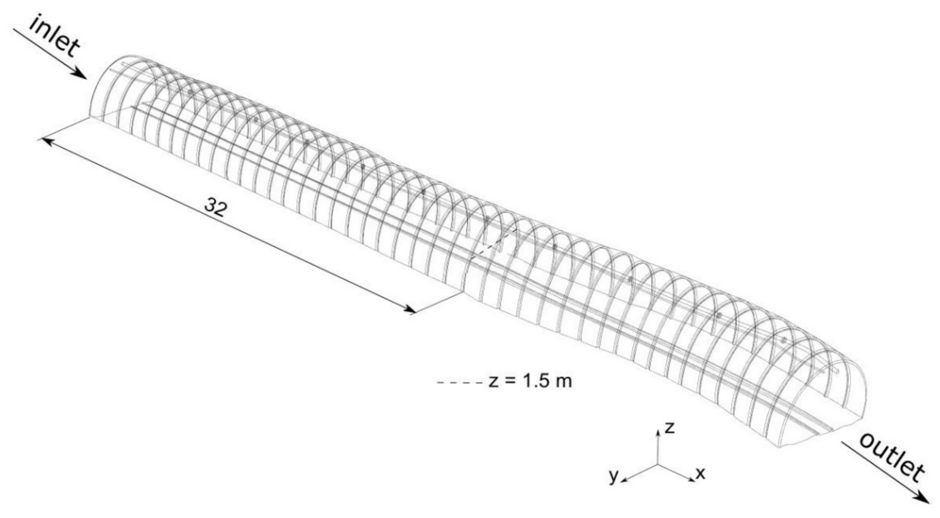
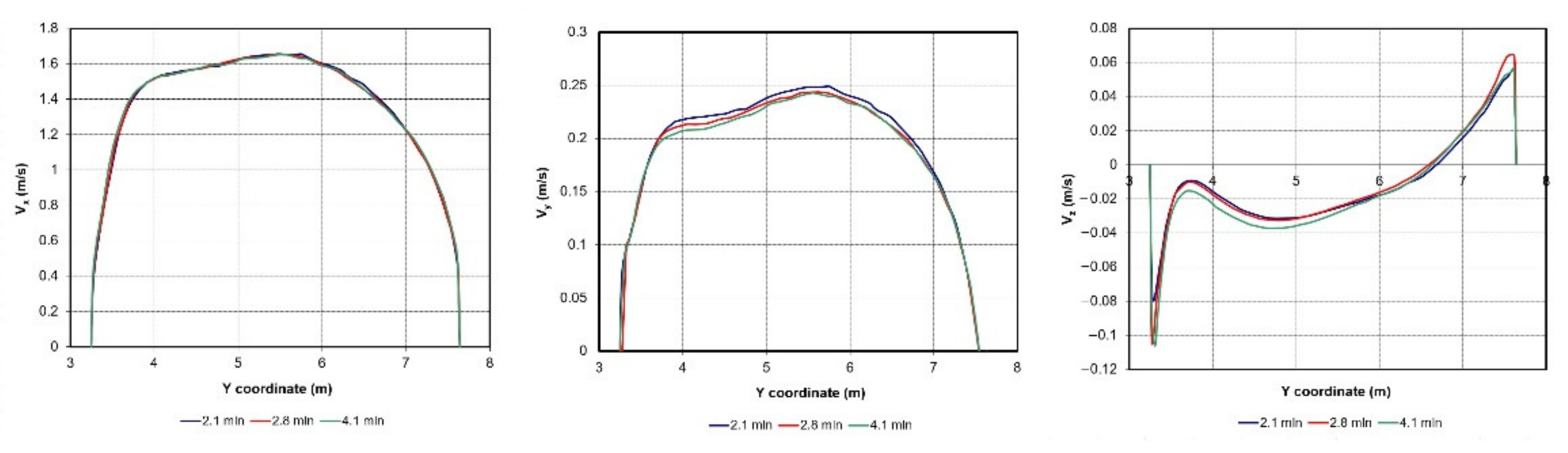
For the grid sensitivity study, a shorter section of the gallery, containing the first 32 m plus a 17 m long part-length of the bend, was considered. This section had properties that were representative of the whole domain, but was considerably shorter, which facilitated the denser grid calculations. The coarser grid model consisted of 9.7 million tetrahedral cells, and after conversion to a polyhedral grid, the number of cells went down to 2.1 million. The second model consisted of 13 million tetrahedral cells; after conversion, there were 2.8 million polyhedral cells. The third grid model consisted of 22.2 million tetrahedral cells, and after conversion, there were 4.1 million polyhedral cells. The velocity components V_x, V_y and V_z at the measuring line at height z = 1.5 m were used for the comparison of solutions. The measuring line was situated 32 m behind the inlet to the numerical model, at the place of installation of measuring Position II (Figure 9).

An example of the velocity comparison is shown in Figure 10 The low differences of values for the 4.1 million and 2.8 million cell models justify the selection of the second model’s grid density.

5. Comparison of Numerical Simulation Results with Results of Velocity Profile Shape Measurements

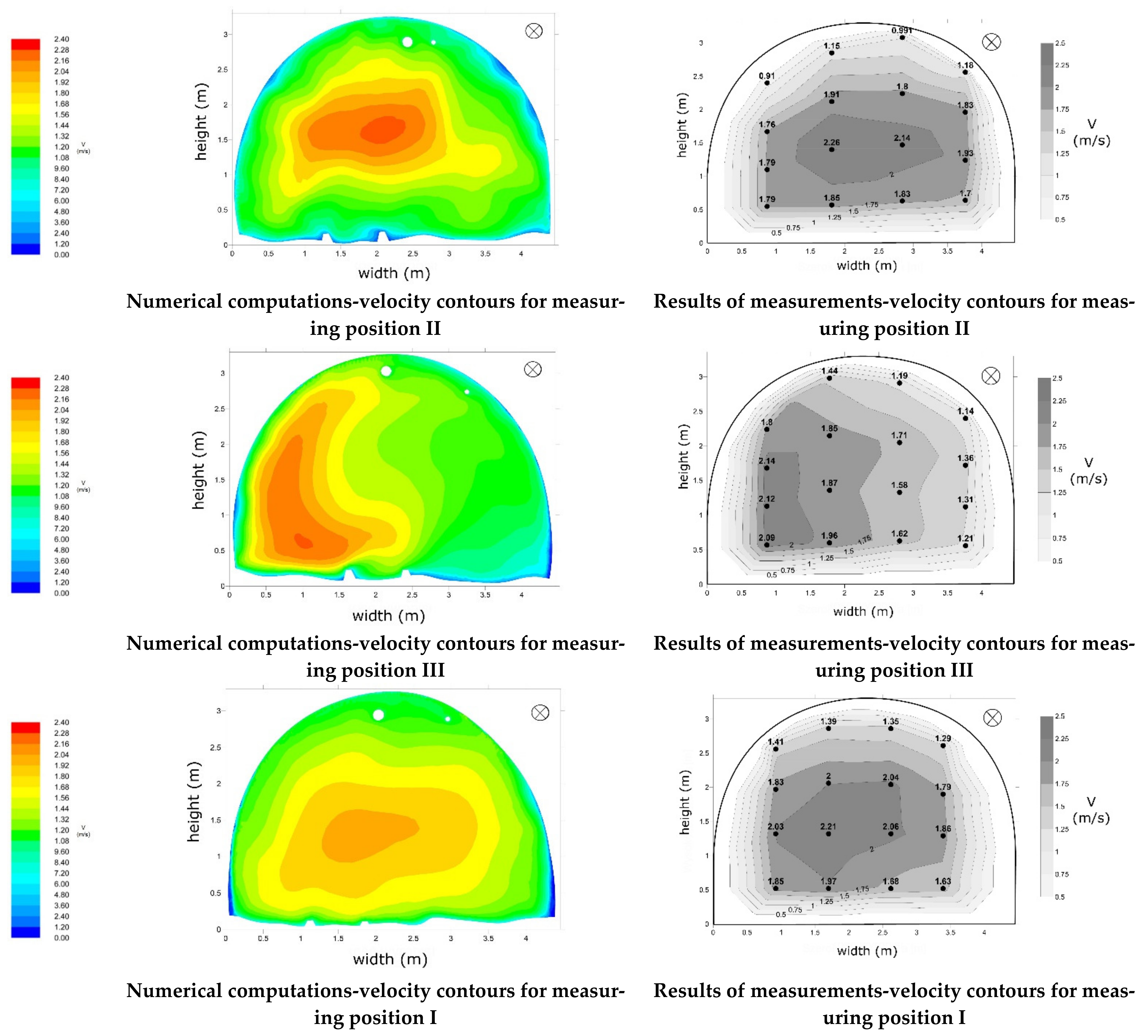
The obtained results of numerical computations and the results of measurements in the mine gallery are presented in the form of velocity profile contours for individual measuring positions. In addition, the values of average velocities (obtained from measurements and CFD computations) are presented in a tabular form for each measuring point (corresponding to the anemometer position in the measuring cross-section) for individual measuring positions.

To present a quantitative assessment of the precision measure of the numerical simulations, a decision was made to use a relative error measure [22]:

$$\delta =\frac{\Delta x}{x}\cdot 100\%=\frac{\left|x-x_0\right|}{x}\cdot 100\%$$

(8)

where:

• x—measured quantity;
• x₀—quantity computed numerically.

An average relative error for the entire measuring cross-section is calculated as a sum of relative errors at individual measuring points divided by the number of measuring points:

$${\delta }_{śr}=\frac{1}{n}{\displaystyle {\sum }_{i=1}^n\frac{\left|x-x_0\right|}{x}}\cdot 100\%$$

(9)

where:

• n—number of measuring points in the cross-section.

The results of numerical computations show a high qualitative and quantitative convergence as compared with the measurement results for all three measuring cross-sections.

The recorded values of average air flow velocities at measuring Position II present a developed velocity profile, which is confirmed by the velocity profile obtained by means of numerical computations (Figure 11). The mean relative error, being a comparison of measurement results with numerical computations, for measuring Position II is 14.85% (Table 2).

For measuring Position III, situated behind the bend, the air flow due to the action of inertial force sticks to the outer wall of the bend, resulting in the origination of vortices and flow recirculation zones at the opposite wall (Figure 11). Because of this, in both the measurement results and the numerical computation results, it is possible to observe the location of the highest velocities, situated approx. 1 m from the left wall. The obtained mean value of relative error for measuring Position III is 10.93% (Table 2).

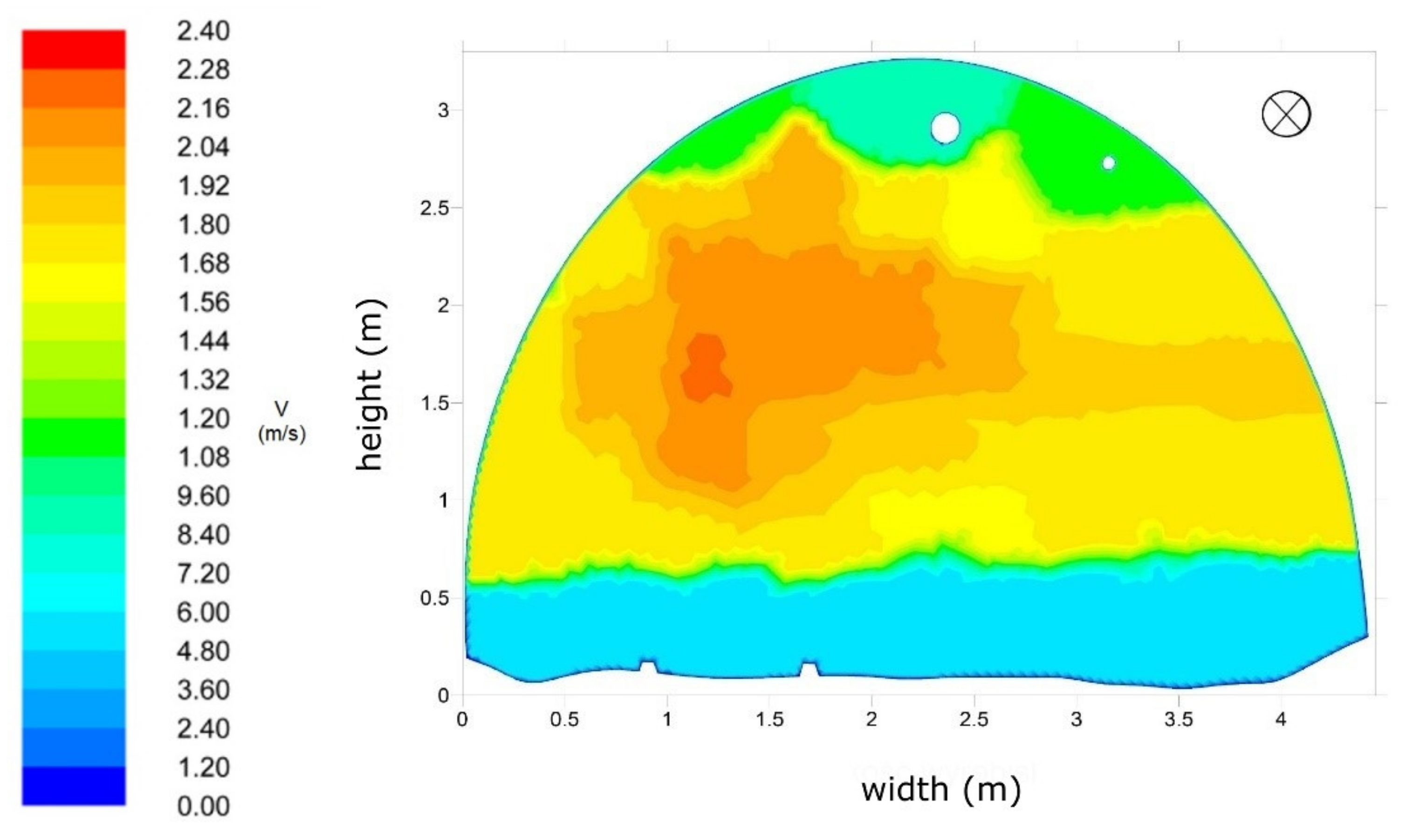
In the case of Position I, the velocity contours obtained from numerical computations are made in the cross-section plane situated 56.0 m behind the bend outlet. The analysis of the measurement results shows a reshaping of the velocity profile, but the effect of the bend in the form of a slight asymmetry is still visible. The largest velocity range was recorded in the central part of the gallery cross-section (Figure 11). The results of numerical simulation reflect the shape of the velocity profile, which is also confirmed by a mean relative error equal to 9.73% (Table 2).

6. Conclusions and Discussion

The paper presents a broad range of performed work aimed at the numerical modelling of turbulent air flow in a section of a mine gallery. This comprised air flow velocity measurements in the mine gallery and the use of modern measuring techniques to accurately represent the shape of the gallery. All of the undertaken actions led to the most precise possible acquisition of the information that was necessary to carry out numerical simulations in a mine environment.

Measuring data acquired from the Multi-Point Velocity Field Measurement System (SWPPP), allowing simultaneous measurement of flow velocity at sixteen measuring points of a mine gallery cross-section, were used to determine boundary conditions and to verify simulations. The database was acquired in this way, containing results of instantaneous measurements and of average air flow velocities at individual measuring points for three measuring positions, as well as velocity profiles obtained through estimation.

In addition, to design an accurate representation of the shape of the mine gallery in which the flow velocity measurements were carried out, a decision was made to use the laser scanning technique. Based on the performed measurements of the shape of the mine gallery, a geometrical model was designed, with this being a copy of the actual model, taking into consideration the existence of a hydraulic pipe and a pipeline in the vicinity of the roof, floor unevenness, and deformations of individual arches of the support.

A numerical model for the simulation of non-stationary turbulent air flow was developed based on the obtained data. The finite volume method was used in simulations. Target simulations were preceded with a grid sensitivity study. A sequence of case studies used several turbulence models, starting from the classical k-e, through k-w SST, and ending with the SAS model, which provided the best fit to the field measurements. The obtained results of numerical computations show a high qualitative and quantitative convergence as compared with measurement results. The obtained velocity profiles for all three measuring positions represent the shape of profiles obtained by means of vane anemometers. A quantitative analysis—the analysis of the results of the average air flow velocity measurements for measuring points—shows a small mean error. The highest mean error between the measurement and numerical computation results is 14.85%, while the smallest is 9.73%. Discrepancies are comparable with the velocity measurement uncertainty, estimated at approx. 10% for flows featuring such significant fluctuations.

The results presented in this paper provided a point of reference for studies carried out by J. Janus [23] on the influence of simplifications of geometrical representation of the computational area on the precision of simulation results. In particular, it turned out that the impact of neglecting the presence of pipelines, floor unevenness and cross-section fluctuations causes a dozen or so percent deterioration of the accuracy of the obtained results. Determination of the velocity profile at the inlet is more important for simulation accuracy. This issue will be the subject of further analyses.

A 3D scanner was used to generate a cloud of points determining the shape of gallery walls. Hand-held scanners may be used for this, which substantially accelerate and simplify the scanning. However, the problem of point cloud conversion into a shape that is useful for computational grid generators remains. A computational grid with centimeter sizes corresponds to the flow conditions in galleries. The data from the point cloud should be filtered, removing details that are insignificant for the flow modelling. So far, the presence of support ribs has practically made automation of this process impossible. This issue requires further work, perhaps with the use of artificial intelligence to distinguish the ribs.

Data on a single velocity component at a few dozen points were obtained in field measurements. These provide a rough outline of velocity profiles. They do not, however, provide sufficient information about fluctuation components and flow phenomena in the vicinity of walls. These issues are the subject of a separate study using hot wire probes for the velocity vectors and fluctuation component measurements [24]. Implementation of their results may further improve the quality of numerical modelling.

The point cloud data may also be used for building scale models with additive manufacturing technologies (3D printing). These models may be used for laboratory experiments. In laboratory conditions, far more informative PIV velocity field measurement methods may be applied [25].

References

- De Souza, A. How to—Understand Computational Fluid Dynamics Jargon; NAFEMS Ltd.: Hamilton, UK, 2005. [Google Scholar]
- Wala, M.A.; Vytla, S.; Taylor, C.D.; Huang, G. Mine face ventilation: A comparison of CFD results against benchmark experiments for the CFD code validation. Min. Eng. 2007, 59, 49–55. [Google Scholar]
- Ren, T.; Balusu, R. The Use of CFD modelling as a tool for solving mining health and safety problems. In Proceedings of the 10th Underground Coal Operators’ Conference, Sydney, Australia, 23–24 November 2010. [Google Scholar]
- Wang, Z.; Ren, T.; Ma, L.; Zhang, J. Investigations of Ventilation Airflow Characteristics on a Longwall Face—A Computational Approach. Energies 2018, 11, 1564. [Google Scholar] [CrossRef] [Green Version]
- Luo, Y.; Zhao, Y. Field and experimental research on airflow velocity boundary layer in coal mine roadway. Arch. Min. Sci. 2020, 65, 255–270. [Google Scholar] [CrossRef]
- Branny, M.; Karch, M.; Wodziak, W.; Jaszczur, M.; Nowak, R.; Szmyd, J. An experimental validation of a turbulence model for air flow in a mining chamber. J. Phys. Conf. Ser. 2014, 530, 012029. [Google Scholar] [CrossRef] [Green Version]
- Wierzbiński, K. Wpływ geometrii chodnika wentylacyjnego i sposobu jego likwidacji na rozkład stężenia metanu w rejonie wylotu ze ściany przewietrzane sposobem U w świetle obliczeń numerycznych CFD. Zesz. Nauk. Inst. Gospod. Surowcami Miner. Energią Pol. Akad. Nauk 2016, 94, 217–228. [Google Scholar]
- Janus, J. Construction the numerical models geometry by using terrestrial laser scanning. In Selected Issues Related to Mining and Clean Coal Technology; AGH: Kraków, Poland, 2016; pp. 235–242. [Google Scholar]
- Janus, J. Assessment of the possibilities of using laser scanning for numerical models constructions. Trans. Strat. Mech. Res. Inst. 2016, 18, 27–34. [Google Scholar]
- Warneke, J.; Dwyer, J.G.; Orr, T. Use of a 3-D scanning laser to quantify drift geometry and overbreak due to blast damage in underground manned entries. Presented at the 1st Canada—U.S. Rock Mechanics Symposium, Vancouver, BC, Canada, 27–31 May 2007. [Google Scholar]
- Bouchiba, H.; Santoso, S.; Deschaud, J.-E.; Rocha-Da-Silva, L.; Goulette, F.; Coupez, T. Computational fluid dynamics on 3D point set surfaces. J. Comput. Phys. X 2020, 7, 100069. [Google Scholar] [CrossRef]
- Menter, F.R.; Egorov, Y. A scale adaptative simulation model using two equations models. In Proceedings of the 43 AIAA Aerospace Sciences Meeting and Exhibit, Reno, NV, USA, 10–13 January 2005. [Google Scholar]
- Walentek, A. Analysis of the applicability of the convergence control method for gateroad design based on conducted underground investigations. Arch. Min. Sci. 2019, 64, 765–783. [Google Scholar] [CrossRef]
- Sokoła-Szewioła, V.; Wiatr, J. Application of laser scanning method for the elaboration of digital spatial representation of the shape of underground mining excavation. Przegląd Górniczy 2013, 8, 206–211. [Google Scholar]
- Krach, A.; Krawczyk, J.; Kruczkowski, J.; Pałka, T. Variable of the Velocity Field and Volumetric Flow Rate in Air Ways of Underground Mines. Arch. Min. Sci. 2006, 1. [Google Scholar]
- Martikainen, A.L.; Dougherty, H.N.; Taylor, C.D.; Mazzella, A.L. Sonic anemometer airflow monitoring technique for use in underground mines. In Proceedings of the 13th U.S./North American Mine Ventilation Symposium, Sudbury, ON, Canada, 13–16 June 2010; pp. 217–224. [Google Scholar]
- Kruczkowski, J.; Ostrogórski, P. Metanoanemometr SOM 2303: Nowoczesne Metody Zwalczania Zagrożeń Aerologicznych w Podziemnych Wyrobiskach Górniczych; GIG: Katowice, Poland, 2015; pp. 117–127. [Google Scholar]
- Cardwell, N.D.; Vlachos, P.P.; Thole, K. Developing and fully developed turbulent flow in ribbed channels. Exp. Fluids 2011, 50, 1357–1371. [Google Scholar] [CrossRef]
- Ansys Inc. Ansys Fluent Theory Guide; Ansys Inc.: Canonsburg, PA, USA, 2019. [Google Scholar]
- Ligęza, P.; Poleszczyk, E.; Skotniczny, P. Method and the system of spatial measurement of velocity field of air flow in a mining heading. Arch. Min. Sci. 2009, 54, 419–440. [Google Scholar]
- Skotniczny, P.; Ostrogórski, P. Three-dimensional air velocity distributions in the vicinity of a mine heading’s sidewall. Arch. Min. Sci. 2018, 63, 335–352. [Google Scholar] [CrossRef]
- Roszkowski, W.; Trutwin, W.; Wacławik, J. Mine Ventilation Measurements; Wydawnictwo “Śląsk”: Katowice, Poland, 1992. [Google Scholar]
- Janus, J. Numerical Modeling of Flow Phenomena in Mine Drifts Using the Results of Terrestrial Laser Scanning. Ph.D. Thesis, Strata Mechanics Research Institute of the Polish Sciences Academy, Kraków, Poland, 2018. [Google Scholar]
- Skotniczny, P.; Ostrogórski, P.; Krawczyk, J.; Janus, J. Determination and acquisition of parameters which characterize the turbulent flow in vicinity of sidewall in deep coal mine. Trans. Strat. Mech. Res. Inst. 2018, 21, 61–73. [Google Scholar]
- Kumar, A.; Arya, S.; Wedding, W.C.; Novak, T. Examination of Capture Efficacies of a Shearer Mounted Flooded Bed Dust Scrubber Using Experiments and Computational Fluid Dynamics (CFD) Modelling on a Reduced Scaled Model. In Proceedings of the 16th North American Mine Ventilation Symposium, Golden, CO, USA, 17–22 June 2017; pp. 20-1–20-8. [Google Scholar]