Applying Endogenous Learning Models in Energy System Optimization

Abstract

Conventional energy production based on fossil fuels causes emissions that contribute to global warming. Accurate energy system models are required for a cost-optimal transition to a zero-emission energy system, which is an endeavor that requires a methodical modeling of cost reductions due to technological learning effects. In this review, we summarize common methodologies for modeling technological learning and associated cost reductions via learning curves. This is followed by a literature survey to uncover learning rates for relevant low-carbon technologies required to model future energy systems. The focus is on (i) learning effects in hydrogen production technologies and (ii) the application of endogenous learning in energy system models. Finally, we discuss methodological shortcomings of typical learning curves and possible remedies. One of our main results is an up-to-date overview of learning rates that can be applied in energy system models.

1. Introduction

It is by now well known that conventional energy production based on fossil fuels cause problematic CO₂ emissions that contribute to global warming. (Herein, we take energy production to mean the conversion of primary energy sources—potential energy in oil or uranium, kinetic energy in wind, etc.—into energy carriers that are convenient for storage or transport—electricity, hydrogen, etc. Similarly, energy consumption refers to the utilization of these carriers—to power electronics, transport people and goods, etc.) Avoiding a climate crisis requires a worldwide effort to reduce such greenhouse gas emissions, and the EU has set its target to be net-zero emissions by 2050 [1]. Since the energy system accounts for approximately 80% of the greenhouse gas emissions in the EU [2], most of this burden falls to the energy sector. Some reduction is expected from energy efficiency increases and the circular economy, but the majority must likely come from investments in novel energy technologies: renewable electricity, biofuels, hydrogen as an energy carrier, carbon capture and storage, etc. In this context, energy system models, which attempt to forecast and optimize the entire energy system in, e.g., the EU, are powerful tools for guiding policymakers and minimizing transition costs. Moreover, their cost predictions can be useful for analyzing the competing technologies within a sector. As examples, the TIMES model generator [3] is used globally in providing guidance regarding future policies, while the PRIMES model [4] is used by the European Commission in long-term strategies such as “A Clean Planet for all” [5].

One fundamental challenge for such energy system models is that one requires estimates for the costs of every relevant energy technology within the investigated timeframe. However, the investment required to, e.g., build and operate one new power plant can change drastically from 2020 to 2050: costs typically decrease as a new technology matures and becomes more widely deployed, but they can also increase due to changes in raw materials or regulations resulting in more stringent safety protocols. These costs are especially important for renewable energy technologies, as their cost of electricity is dominated by the capital costs and are not affected by fossil fuel prices. Samadi [6] provides a broad overview of the factors that typically influence the costs of electricity generation. He groups these into four main clusters: learning and technological improvements, economies of scale, changes in input factor prices, and social and geographical factors. Within the context of energy system models, the first two clusters are especially important as these can be directly affected by variables in the model.

Changes in technology costs due to learning effects can be implemented either exogenously [7] or endogenously [8] in an energy system model [9]. Exogenous learning means that one models the technology cost purely as a function of time, independent of any investment choices made during the energy system optimization. In other words, the technology cost forecast can be regarded as an input to the model. They are frequently obtained from in-depth analysis of the individual energy technologies. Conversely, endogenous learning means that the costs are assumed to be some function of the prior investments, and they change dynamically as the energy system optimization routine explores different investment choices. Thus, the technology cost forecast is an output from the energy system optimization. This is clearly a more realistic scenario, and it avoids some pitfalls associated with the exogenous learning models. For instance, in the exogenous case, an investment algorithm may choose to delay all investments for a decade, since the technology cost will have decreased by then, while in the endogenous case, the costs of a new technology do not decrease unless someone invests in the technology. The main drawback of this strategy is that endogenous learning causes the optimization problem to become nonlinear, requiring more advanced and computationally expensive solution algorithms than exogenous learning. Furthermore, problems may arise with learning occurring outside the investigated bounds of the energy system models, resulting in higher costs within the model than in reality. This necessitates adjustments of the learning rates.

To provide a realistic pathway to a zero-emission future, energy system modeling including learning effects can be a useful planning tool. Moreover, hydrogen is increasingly considered as an important part of such a zero-emission energy system, assuming that hydrogen is produced via a process with no or low greenhouse gas emissions. However, there is currently a lack of reviews that summarize the available research on learning effects in hydrogen production, presenting a difficulty for incorporating these effects into energy system models. The aim of this publication is precisely to investigate learning rates for hydrogen production and to focus on the implementation and implications of the endogenous learning approach in energy system models. The review is structured as follows. We provide a conceptual introduction to endogenous learning models in Section 2, focusing on learning-by-doing and learning-by-research effects in particular. In Section 3, we present the results of a thorough literature review, where we investigated what learning rate data for energy technologies are publicly available. A key focus in this area is to also include technologies outside the typical electricity generation technologies. Finally, we conclude with a discussion of problems with endogenous cost reductions in Section 4.

2. Cost Development in Technologies

There exist different strategies for estimating the future costs of a technology [10]. These can broadly be categorized as “bottom–up estimates”, based on state-of-the-art research and engineering combined with detailed domain knowledge for the calculation of an n’th-of-a-kind (NOAK) plant; “top–down estimates”, based on extrapolating purely empirical trends; as well as combinations of these, as suggested by Rubin [10] and discussed by Roussanaly et al. [11]. The following sections provide an overview of the mathematical concept of top–down estimates via learning curves.

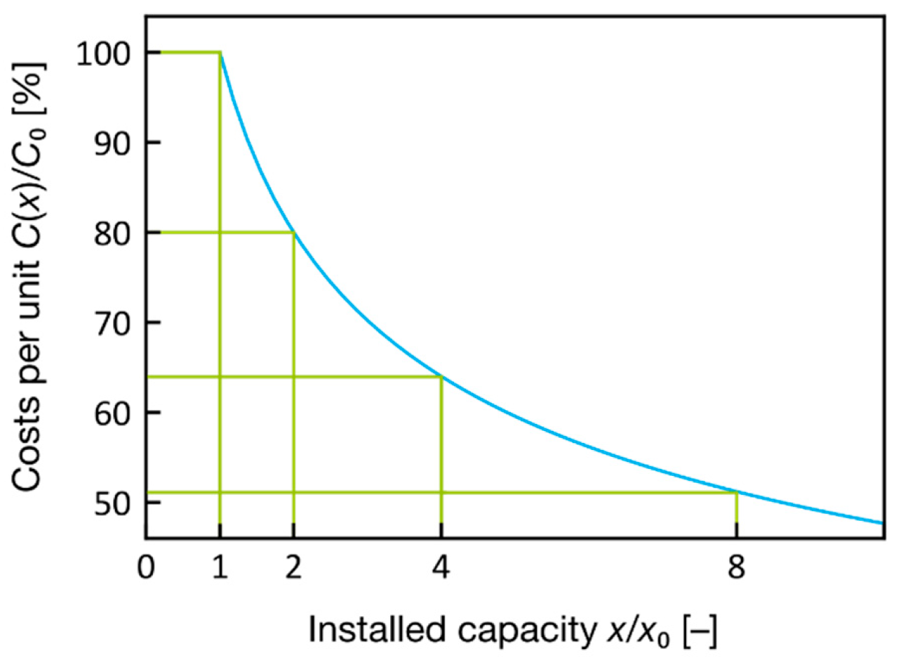
Introduction to Learning Curve Models

The concept of a learning curve or experience curve was originally introduced by Wright [12]. He observed that every time the total number of aircraft that had been produced doubled, the number of person-hours needed to produce one more aircraft had decreased by 20%. This effect is now known as learning-by-doing (LBD) in economics. The same trend was later found to hold not just within one company but for entire industries, and not just in manufacturing, but also for other industries such as energy production [13].

The method originally introduced by Wright is now known as the one-factor learning curve model. Mathematically, it is formulated as follows [14]:

$$C\left(x\right)=C_0{\left(\frac{x}{x_0}\right)}^{b_{\mathrm{lbd}}}.$$

(1)

In Wright’s example, $C\left(x\right)$ measured the cost of producing one airplane after a total of $x$ airplanes have been produced, while $C_0$ and $x_0$ were the corresponding values at some earlier reference time $t_0$. The exponent $b_{\mathrm{lbd}}$ is usually parametrized via a learning rate $\mathrm{LR}=1-2^{b_{\mathrm{lbd}}}$, which describes the cost reduction obtainable by doubling $x$. (If we have an initial capacity $x_0$, and double this $n$ times to get $x=2^n{x}_0$, then a one-factor learning curve yields $C=C_0{\left(x/x_0\right)}^{b_{\mathrm{lbd}}}=C_0{\left(2^n\right)}^{b_{\mathrm{lbd}}}=C_0{(2^{b_{\mathrm{lbd}}})}^n.$ Substituting in the definition $2^{b_{\mathrm{lbd}}}=1-\mathrm{LR}$, we obtain $C=C_0{\left(1-\mathrm{LR}\right)}^n$. This shows that the cost indeed decreases by a fraction $\mathrm{LR}$ for each of the $n$ doublings in capacity that occurs.) In Wright’s example, $\mathrm{LR}=20\%$; generally, it is determined by fitting historical data to Equation (1). See Figure 1 for a visualization of this one-factor learning curve. Note that this learning curve is only valid for technologies that have already been commercialized; until that point, the cost does not generally follow this curve, and it may initially even increase with time [10,11]. To remedy this, some sources use a constant estimate $C\left(x\right)=C_0$ when modeling capacities $x<x_0$ [15], where $x_0$ is an estimated production threshold before learning starts.

The simple one-factor approach outlined above may result in the incorporation of factors independent of the installed capacities into the learning rates (LRs). This may result in both over- and underestimation of the associated LRs. For a concrete example: both private companies and public institutions spend a lot of resources on research and development (R&D), which should reduce technology costs over time. This is often called learning-by-research (LBR) and is a distinct effect from the LBD effect discussed above [9], as it scales with the research budget and not the production or capacity. However, if one fits a one-factor model to the historical cost development, then all cost reductions due to R&D investments will be attributed to LBD in the model, resulting in an overestimation of the LBD effect. If the research budget and production rate are strongly correlated, this is mainly a philosophical issue; in that case, the one-factor model would retain its predictive power as one extrapolates from empirical data. However, if the research budget and production rate change differently with time, one might expect more accurate predictions if the LBD and LBR effects are modeled separately. Such an extended two-factor model can be expressed as [9]:

$$C\left(x, y\right)=C_0{\left(\frac{x}{x_0}\right)}^{b_{\mathrm{lbd}}}{\left(\frac{y}{y_0}\right)}^{b_{\mathrm{lbr}}}$$

(2)

where $y$ corresponds to the R&D spending and $b_{\mathrm{lbr}}$ represents the corresponding LBR parameter. Rubin et al. [9] concluded based on a literature review that R&D can significantly reduce the costs in all stages of technology development. Following the same pattern as above, one can continue to extend the learning curve concept to an arbitrary multi-factor model with independent LRs for each factor included. While multi-factor models are theoretically appealing, in practice, one-factor learning curves are more used due to a lack of available data [9].

Both the one-factor and two-factor learning curves can be generalized to component-based learning curves, also known as composite learning curves. In these models, a “unit” is decomposed into its constituent parts, and then, each of these parts is allowed to evolve according to a different LR. As an example, consider hydrogen production using natural gas reforming with carbon capture and storage. The overall system consists of a reforming section, a hydrogen purification section, a CO₂ capture and processing section, a CO₂ transport section, and a CO₂ storage section. Each section has its own maturity and potential cost reductions through increasing the production capacity. This can either be solved using a composite LR, where the learning associated with each component is aggregated into a single effective LR, or by using individual LRs. The former may result in wrong assumptions on the overall LR through an omitted variable bias [16]. The latter requires the utilization of composite learning curves, which for a one-factor model is [9,17]:

$$C\left(x_1, \dots ,x_N\right)={\displaystyle \sum }_{n=1}^N{C}_n\left(x_n\right)={\displaystyle \sum }_{n=1}^N{C}_{0,n}{\left(\frac{x_n}{x_{0,n}}\right)}^{b_{\mathrm{lbd},n}}$$

(3)

where $C$ is the total cost, $C_n$ is the cost of the n’th component, and $x_n$ is a corresponding production or capacity. This approach also makes it possible to model spillovers from other technologies, by referring to the same component $x_n$ in multiple cost calculations. One example of such spillovers is given by fuel cell electric vehicles and electric vehicles where battery and electric drive train costs are common in both type of vehicles [18]. Another relevant example is photovoltaics, where much of the historical improvements can be attributed to technology spillover from the semiconductor electronics industry.

The simplest version of the component approach discussed above is to only distinguish between components with significant learning effects ($b_{\mathrm{lbd},n}\gg 0$) and negligible learning effects ($b_{\mathrm{lbd},n}\approx 0$). Then, the former is used to calculate a composite LR $b_{\mathrm{lbd}}$ for the fraction $\alpha$ of the initial costs that have significant learning effects. The remaining fraction $1-\alpha$ of the initial costs will remain constant and thus over time become the dominant contribution to the total cost. Mathematically, such a model can be written as:

$$C\left(x\right)=C_0\left[\left(1-\alpha \right)+\alpha {\left(\frac{x}{x_0}\right)}^{b_{\mathrm{lbd}}}\right]$$

(4)

In general, a combination of multi-component and multi-factor analyses yields a sum over contributions from different components, where the cost of each component is now a product of cost-decreasing factors [19]. Each of these factors (LBD, LBR, etc.) has a separate LR that must be estimated based on data. Estimating the uncertainty can also become more complex, since the LRs are often correlated and not independent. Thus, a key problem of both composite learning curves and multi-factor approaches is the availability of data that can be used for obtaining these learning parameters without overfitting as well as the quality of the available data.

A recent review paper by Thomassen et al. [20], which focused on using learning curves for technology assessment and how to incorporate environmental concerns in these models, also touched upon multi-component multi-factor learning curves. They formulated a set of recommendations for how to best apply such learning curves in practice. These included the following suggestions: combining LRs at the component and product levels; combining extrapolated empirical data with expert estimates; and using a tier-based method with quality criteria to evaluate the learning curves.

There are many ways to define $C$ and $x$ in Equation (1). In the context of energy system modeling, the cost variable $C$ usually refers to a relative cost (e.g., €/kW or €/unit) or levelized cost of energy (LCOE), while the experience variable$x$ refers to installed capacity (GW), installed number (units), or total production (TWh of energy production). Learning curves are also used to describe other developments, such as operating efficiency [21] and consumption of individual input factors in production [22]; however, this study is limited to the cost-related applications of learning curves due to their prevalence in energy system models.

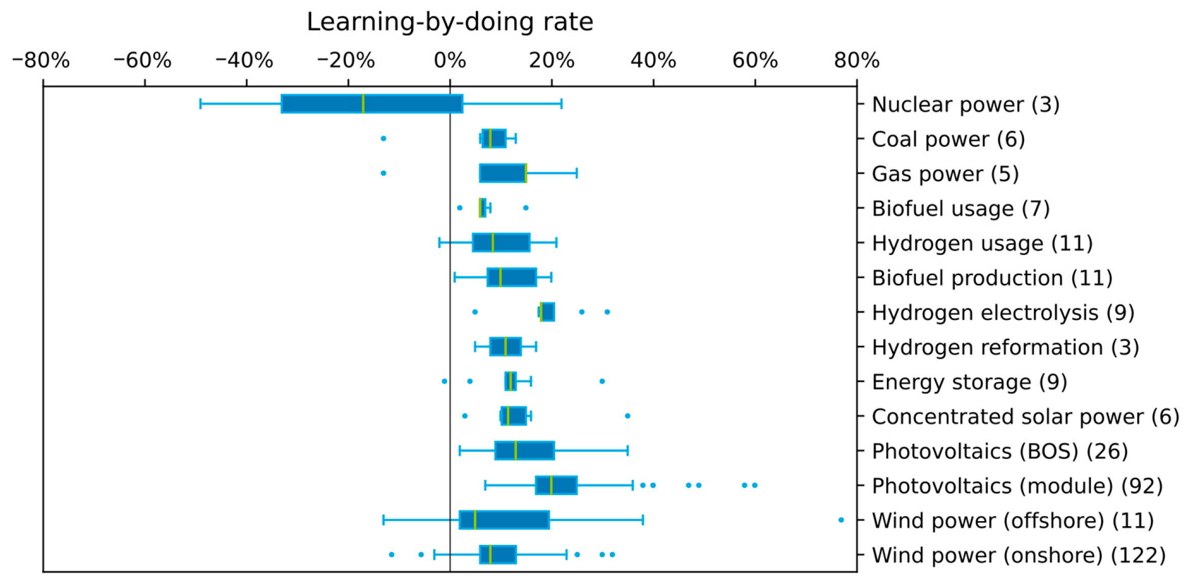
3. Literature Review Related to Learning-by-Doing

LBD effects have been extensively studied for the technologies present in an energy system. It is not surprising that especially onshore wind and solar photovoltaics have received significant attention due to their importance in a low-carbon energy system and their high growth rate in recent years. Figure 2 provides an overview of LBD LRs collected in the current review. As the figure illustrates, there is a significant spread between LRs reported in the literature, although statistical analysis narrows down the intervals. This holds even if there are a large number of publications analyzing a specific technology. Even so, the uncertainty in LR can often be as large as the value of LR, which can have drastic effects on energy system models given that LR affects the learning curve exponent.

There are several reasons for the high spread in LRs. One is that different studies may use different experience variables (e.g., cumulative capacity vs. cumulative production), different cost variables (e.g., plant costs vs. levelized costs), or correct for different confounding variables (e.g., plant locations, plant sizes, material prices). Another is that LRs may inherently differ between geographical regions and time periods, for example due to different regulations. Therefore, it is important that the modeler is aware of these factors and picks the data that most closely corresponds to their chosen scenario. In the tables of Appendix C, the data behind Figure 2 is listed in more detail, including what cost variables, experience variables, regions, and time periods correspond to which individual data points, along with literature references. The remaining uncertainty in LRs should ideally be handled via sensitivity analysis. For instance, it is possible to use the first and third quartiles of the LR distribution as “pessimistic” and “optimistic” sensitivities around the appropriate base case (e.g., the median LR). Related discussions of sensitivity analysis in the context of energy systems and learning curves can be found in Refs. [11,23].

Note that one-factor learning curves do not just pick up actual learning but aggregate everything that historically influenced costs during capacity expansions. This gives rise to some perhaps surprising results, such as negative LRs for nuclear energy in Figure 2. Typically, negative LRs signify changing technology requirements [11], which for nuclear energy can be attributed to e.g., increased safety requirements during its period of rapid capacity doubling in the 1970s [6,16]. It is also worth noting that these numbers are for industry-wide LRs, which tend to be high for small, mass-produced units (e.g., photovoltaics and onshore wind) and low for large, custom-built units (e.g., nuclear power and offshore wind) [11,16]. When the analysis is restricted to nuclear reactors of similar design that are constructed by the same engineer–architect [24], the firm-level LR can increase to 10–12% [16], emphasizing the benefit of reactor standardization. For a more in-depth discussion of negative learning effects, see e.g., Refs. [11,16].

In the rest of this section, we summarize the results of the literature review, focusing on LRs in (i) hydrogen production technologies and (ii) their application in energy system models. A more in-depth discussion of the literature on electricity-related energy technologies and carbon capture and storage, which expand upon previous reviews by Samadi and Rubin by adding newer references, is delegated to Appendix A and Appendix B.

3.1. Learning-by-Doing in Hydrogen Production

Hydrogen is increasingly considered to be an important energy carrier in a low-carbon energy system [25,26]. Hence, it is important to also include hydrogen production with learning effects in an energy system model to avoid a potential bias. Most studies on learning effects in hydrogen production focus on electrolysis due to its low deployment to date. Hence, significant cost reductions can be expected with increased deployment.

Learning effects for hydrogen production from natural gas have been less investigated. One reason is that much of this hydrogen goes to refineries, ammonia production facilities, and methanol production facilities [27]. In these processes, hydrogen is directly utilized, while the composition of the feedstock may vary. These production processes differ significantly, making it complicated to obtain reasonable LRs. For instance, methanol plants do not maximize their hydrogen yield, as the ideal ratio between hydrogen and carbon monoxide is two for methanol synthesis [27]. The challenges of estimating learning effects for such hydrogen production processes are elaborated in Rubin et al. [28]. They note that complicating factors include differences in feedstocks, plant size, desired hydrogen purity, the possibility of steam export, and economic factors.

One source that did study learning rates for hydrogen production from natural gas was the work by Rubin et al. [15,28]. They considered the process known as steam–methane reforming (SMR), whereby steam and methane undergo a catalyzed reaction at high temperatures to form a mixture of hydrogen and carbon monoxide. Combined with carbon capture and storage (CCS), this process provides one pathway to producing clean hydrogen. Rubin et al. considered such combinations of SMR units with carbon capture and estimated the SMR LR using the hydrogen price as a cost variable C and the globally produced hydrogen as an experience variable x. They assumed that the ratios between energy input, capital charges, and operation and maintenance (O&M) remained constant, while the annual natural gas consumption reduction was 1.1%. Their study concluded with an LR of 27% both for the capital charges and O&M costs.

In another study, Schoots et al. [29] investigated learning effects with respect to hydrogen production technologies. Their study used cost data that goes back to the 1940s and focused on SMR, coal gasification, and alkaline electrolysis. The partial oxidation of oil and naphtha was not included due to limited data quality and the large variety of feedstock. The production capacity was scaled to avoid confusing LBD and economy of scale. They found significant LRs of 11 ± 6% and 18 ± 13% for the investment costs of SMR and electrolysis, respectively. Important factors preventing even higher LRs were improved energy efficiency, stricter environmental regulations, and potentially stricter hydrogen purity requirements. All these effects increase capital costs. However, the production costs were insensitive to learning effects, as most of the production costs are related to energy input in the form of natural gas, coal, or electricity. Further variable costs such as insurance or personnel do not show learning at all. These results cannot directly be compared to the results by Rubin et al., as the basis for the LR is different, and the study accounted for the economy of scale in hydrogen production.

Schmidt et al. [30] performed an expert elicitation study for the future costs of electrolysis and compared the potential future costs proposed by domain experts to the ones obtained via learning curves. They investigated alkaline electrolysis (AEC), proton exchange membrane electrolysis (PEMEC), and solid oxide electrolysis (SOEC). They used an LR of 18% from proton exchange membrane fuel cells for PEMEC due to a lack of data. Similarly, solid oxide fuel cells with an LR of 28% were used as surrogates for SOEC. The reason for using LRs for fuel cells was their similarity to electrolyzers. With two different deployment scenarios, they analyzed the future cost predictions by the experts. These were mostly in line with the LRs and their uncertainties—except for the AEC, where the experts predicted lower costs.

Böhm et al. [19] analyzed electrolyzers via composite learning curves—specifically, via a modified version of Equation (3). Furthermore, spillover effects between electrolyzer types were included for power electronics and gas conditioning. Their analysis showed that a component-based approach reduced the LR as production increased. This was because the initially most expensive components also had the highest LRs, so increased production shifted the cost distribution toward components with lower learning potential. For example, bipolar plates with an LR of 18% represented 51% of the initial cost of a PEMEC; but after 1000 times more cells had been produced, this share had dropped to 24%. The LRs reported for AEC, PEMEC, and SOEC were 19.5%, 17.5%, and 20.5%, respectively at the first stage of deployment. Except for SOEC, these values are similar to the ones reported by Schmidt et al. [30]. Krishnan et al. [31] reported an LR of 16 ± 6% for AEC, which is also similar to the other values.

Haltiwanger et al. [32] investigated a different production route through a Zn/ZnO thermochemical cycle and concentrated solar power (CSP). As there exists no reliable cost data for the reactor for the cycle, SMR data from Rubin et al. [15] were used as a surrogate. The data for the CSP section were obtained by splitting the cost for a CSP plant into a steam cycle section and the solar components. The cumulated LR was calculated as 13–23% with the levelized cost of hydrogen as the cost basis and the cumulative hydrogen production as the capacity basis. This study was later extended to compare the solar thermochemical cycle to photovoltaic with electrolysis with composite LRs allowing different growth rates in photovoltaics and electrolyzers, as well as the Zn/ZnO cycle and the CSP plant [17]. In this study, the thermochemical cycle was modeled with an LR of 19 ± 8%. This was based on a prior study of 108 different data sets from 22 industrial sectors [33], which concluded that the LR was normally distributed with a mean of 19% and standard deviation of 8%.

3.2. Application of Learning-by-Doing in Energy System Models

As shown in Section 2, LBD requires the implementation of nonlinear, nonconvex functions. Most energy system models are either formulated as linear problems or mixed-integer linear problems. The former formulation does not allow learning curves and must rely on exogenous learning approaches. Mixed-integer linear problems allow implantation through an approximation as piecewise linear functions for the cumulative cost as is the case, e.g., in the Endogenous Technological Learning (ETL) extension for the TIMES model [3]. Using the cumulative investment costs furthermore avoids problems with bilinear terms in the objective function. However, this translates the original linear problem into a mixed-integer linear problem, which drastically increases the computational complexity. Therefore, in general, LBD is only implemented in models focusing on specific sections of the energy system, e.g., the power supply section without geographical scope or simple technologies with geographical scope, and not in models focusing on the overall energy system such as TIMES. For an overview of the individual models, we refer to Junginger et al. [34] and Heuberger et al. [14]. From here on, we focus on the impact of endogenous learning on the energy system model results.

Heuberger et al. [14] developed a power capacity expansion model with endogenous learning called ESO-XEL. Technology learning was implemented in the mixed-integer linear programming (MILP) framework as piecewise linear functions via the cumulative cost and not the unit cost, as described in detail by Gómez [35]. MILP refers to optimization problems where (i) all requirements are represented as linear relationships and (ii) optimization is performed with respect to both discrete and continuous variables. This distinction is important, as different classes of optimization problems require different algorithms and computation time. The utilization of cumulative costs avoids nonlinearities in the cost function. The aim of the paper is to analyze capacity expansion in the United Kingdom for a reduction of CO₂ emissions by 2050. The simultaneous global expansion of generation technologies was identified as a problem with a local capacity expansion model using endogenous learning. Hence, they modified the LR to account for the forecasted capacity expansion on a global level. This is especially important for offshore wind expansion due to high initial costs preventing its widespread implementation. However, in general, the installed capacity also depends on the LR. Specifically, assuming learning for carbon capture increased the deployment of fossil power plants with carbon capture compared to the approach with constant prices. This was mostly due to the low installed numbers to date, counterweighing the smaller LR. Heuberger et al. [14] also included a constraint on the maximum capacity expansion for a technology per year, i.e., an implementation speed constraint. This approach avoids an issue where a model may choose an unrealistically large investment in a single technology to minimize costs.

Daggash and Mac Dowell [36] utilized the ESO-XEL model for analyzing how net-negative emissions can be achieved in the power system and what the most cost-effective approach was. To this end, CO₂ direct air capture (DAC) was included with an assumed LR of 9%. Despite having a moderate LR and low existing capacity, which should imply a large potential for LBD, DAC was only utilized in net-negative scenarios when biomass with carbon capture and storage (CCS) was insufficient to remove CO₂ from the atmosphere. Here, the high learning effects did not outweigh the high operational and investment costs of direct air capture. Chen et al. [37] used a similar approach to analyze the impact of bioenergy with CCS in the United Kingdom. As they had a geographically discretized model, more knowledge related to transport chains could be incorporated. Their subsequent sensitivity analysis showed that the LR had a significant impact on the costs of removing CO₂ from the atmosphere. However, due to the focus on biomass supply chains and inclusion of only two technologies, it was not possible to distinguish the results from simulations without learning except for the costs.

Handayani et al. [38] implemented endogenous learning in the LEAP model for analyzing the capacity expansion for the Java–Bali system in Indonesia. Contrary to Heuberger et al. [14], they found that learning was reduced over the course of the model in fixed time frames. In the renewable energy scenario, the maximum amount of fossil energy used was limited. This implied a constraint on how much low-carbon technologies must be included as a minimum. Utilizing LBD influenced the distribution of technologies, but not the total amount of low-carbon energy sources, as coal without carbon capture was still cheaper than renewable energies. Hence, their model selected the minimum allowed number of low-carbon energy sources.

Cerniauskas et al. [39] investigated a supply chain for hydrogen from electrolysis with utilization in both transport and industry in Germany. LRs were assumed for both the electrolyzers (20%, derived from several literature sources, among others Refs. [29,30]), and the hydrogen refueling station (LR of 6%, based on data from AirLiquide). However, the LRs only affected the overall costs, as there was no comparison with different technologies. Hence, conclusions about the effect of LRs with respect to which technology is favorable could not be drawn.

The National Energy Modeling System (NEMS) [40] uses endogenous learning with different learning stages [41]. They differentiated between a revolutionary stage (up to three doublings in capacity), evolutionary stage (three to eight doublings in capacity), and a conventional stage (after eight doublings). Each subsequent stage had a reduction in LR due to the maturity of the technology. Unfortunately, it is not possible to investigate the impact of the implementation on the results of the system, as there is no study analyzing the development of the energy system with and without endogenous cost reductions. Similarly, the Regional Model of Investments and Development (REMIND) [42] used endogenous learning curves in a nonlinear model, although only for solar photovoltaic (PV), concentrated solar power (CSP), wind power, a generalized storage unit, as well as hybrid, electric, and fuel cell vehicles. When comparing different integrated assessment models, it was highlighted that the usage of learning curves resulted in different primary energy usage [43]. However, due to the limitation to certain technologies, it may also have included a bias for the technologies with learning.

The Horizon 2020 project REFLEX [44] implemented LBD within three different models to analyze the development of the future European energy system. Within the model FORECAST, LRs for heating applications showed reduced costs, but its influence on the installation rate was limited, highlighting alternative reasons for choosing specific heating solutions [45]. Contrary, within the model PowerACE, LRs affected the investment in flexible power generators, resulting in a switch from gas turbines and compressed air storage to batteries if the LR for batteries was increased. Similarly, the model ELTRAMOD reduced the installed capacity for gas power with CCS if it was assumed that the CCS components did not experience learning.

4. Discussion of the Implementation of Learning-by-Doing in Energy System Models

Despite their advantages for improving capacity expansion and energy system models, both learning curves in general and LBD in particular face criticism. Samadi [16] divides this criticism into three categories: criticism of the theoretical approach, criticism of the empirical data used, and criticism of the use of LRs.

Criticisms of the theoretical concept refers to the intrinsic limitations of Equation (1). As discussed in Section 2, a one-factor learning curve is precisely that: it attributes all cost reduction to a single factor, LBD. In practice, other sources of cost changes—including learning by research, spillover from experience gained with related technologies, economies of scale, and not least government regulation—may have a major influence on the overall cost of a technology. Thus, due to omitted variable bias, one-factor learning curves tend to exaggerate the importance of experience. In addition, some costs are not necessarily captured in the learning curve data; for instance, technological improvements may reduce pollution or improve energy quality, which may not be reflected in $/kW. Finally, being a top–down empirical method, learning curves are sometimes criticized for being opaque with respect to the underlying mechanisms driving the observed cost reductions.

Criticisms of the empirical data refer to the data sets themselves. Firstly, due to a lack of data availability, price is often used as a surrogate for cost. Although many argue that these should be strongly correlated in a competitive market, this may not always be the case. Moreover, it can often be difficult to discover cost data from a technology that was first deployed. Since this is the phase when most capacity doublings occur, which correspondingly has a strong effect on the empirical learning rate, this may distort results.

Criticisms of the use of learning rates refers to a skepticism of extrapolating past learning rates into the future. Notably, future technology breakthroughs may cause unanticipated periods of rapid learning, while fundamental physical limits on, e.g., material requirements or energy efficiencies may prevent learning past a certain limit. Another point is that learning rate uncertainties are often neglected when applying learning rates in energy system models, while a sensitivity analysis may often be pertinent.

To add to the criticisms above, the following section discusses the form of learning curves and how implementation speed limitations may affect technology selection.

4.1. Unconventional Learning Curves

All publications reviewed so far on LRs and their implementation in energy system models used conventional learning curves, by which we mean that they are treated using one-factor learning curves [Equation (1)] with constant learning rates. However, Yeh and Rubin [13] argue that these learning curves may not accurately model the costs of new technologies. Using as examples flue gas desulfurization and selective catalytic reduction in coal power plants, they show that learning curves behave differently in the early stage. Due to an accelerated deployment of these technologies, the improvements by LBD were reduced in this stage followed by an increase in the LR in subsequent capacity expansion. This would result in an S-shaped curve for the LR. For these two technologies, we can furthermore observe a price increase in the early stage due to problems in scaling up new technologies and wrong estimates. This is irrelevant for commercialized technologies such as wind power and photovoltaics, which already have a high existing capacity. However, it may result in difficulties estimating the real cost for, e.g., large-scale hydrogen production technologies, as both natural gas reforming with CCS and large-scale electrolyzer deployment can be expected to still be in this pre-commercial phase.

A second aspect of S-shaped learning curves is that the LRs level off at a high installed capacity. This seems logical, as prices cannot decrease indefinitely, in which case they would eventually approach zero. Narbel and Hansen [46] utilize a reduction in the LR based on the installed capacity. This is modeled as

$$\mathrm{LR}\left(x\right)={\mathrm{LR}}_0{\left(1-d\right)}^{{\log }_2\left(x/x_0\right)}$$

(5)

where $d$ corresponds to a diminishing rate defined exogenously. This function accounts for reduced learning in future implementations. They use this approach to estimate the costs of different energy scenarios. Correspondingly, the overall costs depend on the chosen diminishing rate. The resulting learning effect may be more reasonable as infinite learning would be unrealistic. On the other hand, the diminishing factor is an additional uncertain model parameter as it is a priori hard to know how much learning is ultimately achievable. Their approach is similar to NEMS [41], where the LR is assumed to be ∼20% for the first three capacity doublings (revolutionary stage), ∼10% for the next five doublings (evolutionary stage), and ∼1% for any further capacity expansions (mature stage).

As outlined in Section 3.1, Böhm et al. [19] used a component learning curve approach that resulted in diminishing electrolyzer LRs as the capacity increased. Intuitively, this occurs because the components with a large LR must diminish in cost fastest, causing technologies with lower LRs to become a larger fraction of the total cost. Figure 3 shows this reduction in the overall LR for the electrolyzer cell stacks. The advantage of the bottom–up modeling from components is a better description of the future costs through accounting for the different LRs in the individual components. Compared to the approach of Narbel and Hansen [46], no assumption for the reduction in learning is applied. This corresponds to the composite learning curve described in Equation (3). However, this approach requires detailed knowledge of both the cost distribution for a technology and the corresponding LRs and still allows a continuous reduction in costs. A similar approach was chosen by Elshurafa et al. [47] for calculating LRs for solar PV systems, as historical data showed a shift in the contribution of the balance of system and the module price on the total price of PV systems.

In their analysis of the Java–Bali electricity system, Handayani et al. [38] considered four ten-year time periods and assumed different LRs for each period. They considered three different scenarios with different assumptions for these LRs; however, they did not compare the study outcome to cases with constant LR across all time periods. The chosen scenario influenced the distribution between the different renewable energy technologies. However, this approach may result in more errors as the prediction of the reduction in the LR is uncertain. Note that the concept itself is similar to the one utilized in NEMS [41]. However, a key difference is that NEMS implements a reduction based on the installed capacity and not the time.

As costs cannot fall indefinitely, another approach is to define a minimum cost to which the learning curve is assumed to converge. The motivation is that material and production costs will at one point be the limit. For instance, Viebahn et al. [48] assume a minimum price for the power block in a CSP plant. A similar approach is taken by Schmidt et al. [30] to calculate the minimum prices of electrical energy storage. Similarly to the previously mentioned problems, the exact value of the minimum cost value is difficult to estimate and may lead to wrong interpretations of the results of an energy system model.

In some cases, there is an inherent uncertainty in the learning curve, which may be difficult to impossible to foresee a priori. One example from Ref. [11] is the case of ethanol production, where the LR appeared to abruptly change from 7% to 29% in 1985, resulting in a piecewise-constant LR providing the best fit to the historical data.

4.2. Implementation Speed Constraints

An implementation speed constraint refers to a maximum capacity expansion per time unit. A physical analogy is the maximum production capacity of, e.g., batteries. LBD favors early cost reductions through investing heavily in technologies with a large LR and a low installed capacity [14]. Hence, it may result in unrealistic composition of the energy system if the implementation speed is not restricted. The estimation of the implementation speed for the foreseeable future is possible due to the knowledge of investment in production capacities and the knowledge of current production capacities. The estimation of the implementation speed in, e.g., the 2040s, is on the other hand difficult due the potential accumulation of production capacities and a correspondingly high uncertainty. This is a common issue with endogenous learning models: one may end up replacing an exogenous cost with an exogenous capacity expansion constraint, thus substituting one exogenous assumption or prediction for another. This is also pointed out by Lolou et al. [3], who mentions that frequently, this bound is an active constraint, raising questions around the advantages of endogenous compared to exogenous learning.

Heuberger et al. [14] estimated the implementation speed as a building rate from historic data showing how fast technologies can be implemented. The building rates of technologies not deployed on a large scale in the UK were estimated from comparable European countries. Due to the uncertainty associated with the building rates, scenarios were conducted with high and low building rates. These scenarios show the impact of the chosen rates on the final power generation and have a significant impact on the cumulative total system cost. The other studies in Section 3.2 do no not mention such a constraint. This can be potentially explained by the limited number of technologies utilized, hence avoiding overinvestment in a single technology for satisfying demand constraints.

5. Conclusions

We have reviewed the available data on LRs for technologies that are expected to be important in future energy systems. Compared to existing reviews, our focus has been on hydrogen production technologies, how endogenous learning models are applied in energy system models, and how the utilization of endogenous learning may affect the model results. Current implementation of endogenous learning models largely focuses on models representing the power sector for individual countries. Certain publications narrow the focus further down to individual value chains. Here, the key aim of endogenous learning is to improve future cost estimates.

However, the application of endogenous learning is still limited in energy system models. Some notable challenges to incorporating endogenous learning in such models include the uncertainty in the LR values, how to include global cost reductions within a local model, and obtaining reasonable estimates for the implementation speed. Considering all these factors, the advantage of using the more realistic approach of endogenous cost reduction may not always outweigh the associated computational costs.

References

1. Von der Leyen, U. A Union that Strives for More: My Agenda for Europe; European Commission: Brussels, Belgium, 2019. [Google Scholar] [CrossRef]
2. Pilzecker, A.; Fernandez, R.; Mandl, N.; Rigler, E. Annual European Union Greenhouse Gas Inventory 1990–2018 and Inventory Report 2020; European Commission: Brussels, Belgium; DG Climate Action: Auderghem, Belgium; European Environment Agency: Copenhagen, Denmark, 2020; p. 997.
3. Lolou, R.; Goldstein, G.; Kanuda, A.; Lettila, A.; Remme, U. Documentation of the TIMES Model—Part 1; IEA Energy Technology Systems Analysis Programme: Helsinki, Finland, 2016; p. 151. [Google Scholar]
4. E3MLab/ICCS. PRIMES MODEL—Detailed Model Description; National Technical University of Athens: Athens, Greece, 2013–2014. [Google Scholar]
5. European Commission. A Clean Planet for All—A European Long-Term Strategic Vision for a Prosperous, Modern, Competitive and Climate Neutral Economy; European Commission: Brussels, Belgium, 2018. [Google Scholar]
6. Samadi, S. A Review of factors influencing the cost development of electricity generation technologies. Energies 2016, 9, 970. [Google Scholar] [CrossRef] [Green Version]
7. Solow, R.M. A Contribution to the Theory of Economic Growth. Q. J. Econ. 1956, 70, 65–94. [Google Scholar] [CrossRef]
8. Romer, P.M. Increasing Returns and Long-Run Growth. J. Political Econ. 1986, 94, 1002–1037. [Google Scholar] [CrossRef] [Green Version]
9. Rubin, E.S.; Azevedo, I.M.L.; Jaramillo, P.; Yeh, S. A review of learning rates for electricity supply technologies. Energy Policy 2015, 86, 198–218. [Google Scholar] [CrossRef]
10. Rubin, E.S. Improving cost estimates for advanced low-carbon power plants. Int. J. Greenh. Gas Control. 2019, 88, 1–9. [Google Scholar] [CrossRef]
11. Roussanaly, S.; Rubin, E.S.; Spek, M.v.d.; Booras, M.; Berghout, G.; Fout, N.; Garcia, T.; Gardarsdottir, M.; Kuncheekanna, S.; Matuszewski, V.N.; et al. Towards improved guidelines for cost evaluation of carbon capture and storage. Zenodo 2021. [Google Scholar] [CrossRef]
12. Wright, T.P. Factors Affecting the Cost of Airplanes. J. Aeronaut. Sci. 1936, 3, 122–128. [Google Scholar] [CrossRef]
13. Yeh, S.; Rubin, E.S. A review of uncertainties in technology experience curves. Energy Econ. 2012, 34, 762–771. [Google Scholar] [CrossRef]
14. Heuberger, C.F.; Rubin, E.S.; Staffell, I.; Shah, N.; Dowell, N.M. Power Generation Expansion Considering Endogenous Technology Cost Learning. Comput. Aided Chem. Eng. 2017, 40, 2401–2406. [Google Scholar] [CrossRef]
15. Rubin, E.S.; Yeh, S.; Antes, M.; Berkenpas, M.; Davison, J. Use of experience curves to estimate the future cost of power plants with CO2 capture. Int. J. Greenh. Gas Control. 2007, 1, 188–197. [Google Scholar] [CrossRef] [Green Version]
16. Samadi, S. The experience curve theory and its application in the field of electricity generation technologies—A literature review. Renew. Sustain. Energy Rev. 2018, 82, 2346–2364. [Google Scholar] [CrossRef] [Green Version]
17. Nicodemus, J.H. Technological learning and the future of solar H2: A component learning comparison of solar thermochemical cycles and electrolysis with solar PV. Energy Policy 2018, 120, 100–109. [Google Scholar] [CrossRef]
18. Anandarajah, G.; McDowall, W.; Ekins, P. Decarbonising road transport with hydrogen and electricity: Long term global technology learning scenarios. Int. J. Hydrog. Energy 2013, 38, 3419–3432. [Google Scholar] [CrossRef]
19. Böhm, H.; Goers, S.; Zauner, A. Estimating future costs of power-to-gas—A component-based approach for technological learning. Int. J. Hydrog. Energy 2019, 44, 30789–30805. [Google Scholar] [CrossRef]
20. Thomassen, G.; Passel, S.v.; Dewulf, J. A review on learning effects in prospective technology assessment. Renew. Sustain. Energy Rev. 2020, 130. [Google Scholar] [CrossRef]
21. International technology roadmap for photovoltaic (ITRPV). Results 2018 including Maturity Report 2019; Allen Institute For AI location: Washington, DC, USA, 2019. [Google Scholar]
22. Görig, M.; Breyer, C. Energy learning curves of PV systems. Environ. Prog. Sustain. Energy 2016, 35, 914–923. [Google Scholar] [CrossRef]
23. Zwaan, B.v.d. Endogenous learning in climate-energy-economic models—An inventory of key uncertainties. Int. J. Energy Technol. Policy 2004, 2, 130–141. [Google Scholar] [CrossRef]
24. Berthélemy, M.; Rangel, L.E. Nuclear reactors’ construction costs. Energy Policy 2015, 82, 118–130. [Google Scholar] [CrossRef] [Green Version]
25. European Commission. A hydrogen strategy for a climate-neutral Europe; European Commission: Brussels, Belgium, 2020. [Google Scholar]
26. Panos, E.; Kober, T. Report on Energy Model Analysis of the Role of H2-CCS Systems in Swiss Energy Supply and Mobility with Quantification of Economic and Environmental Trade-Offs, Including Market Assessment and Business Case Drafts; Paul Scherrer Institute: Villigen, Switzerland, 2020. [Google Scholar]
27. IEA. The Future of Hydrogen; IEA: Paris, France, 2019. [Google Scholar]
28. Rubin, E.S.; Yeh, S.; Antes, M.; Berkenpas, M. Estimating the Future Trends in the Cost of CO2 Capture Technologies; 2006/6; IEA Greenhouse Gas R&D Programme (IEAGHG): Cheltenham, UK, 2006. [Google Scholar]
29. Schoots, K.; Ferioli, F.; Kramer, G.J.; van der Zwaan, B.C.C. Learning curves for hydrogen production technology: An assessment of observed cost reductions. Int. J. Hydrog. Energy 2008, 33, 2630–2645. [Google Scholar] [CrossRef]
30. Schmidt, O.; Gambhir, A.; Staffell, I.; Hawkes, A.; Nelson, J.; Few, S. Future cost and performance of water electrolysis: An expert elicitation study. Int. J. Hydrog. Energy 2017, 42, 30470–30492. [Google Scholar] [CrossRef]
31. Krishnan, S.; Fairlie, M.; Andres, P.; de Groot, T.; Jan Kramer, G. Chapter 10—Power to gas (H2): Alkaline electrolysis. In Technological Learning in the Transition to a Low-Carbon Energy System; Junginger, M., Louwen, A., Eds.; Academic Press: Cambridge, MA, USA, 2020; pp. 165–187. [Google Scholar]
32. Haltiwanger, J.F.; Davidson, J.H.; Wilson, E.J. Renewable hydrogen from the Zn/ZnO solar thermochemical cycle: A cost and policy analysis. In Proceedings of the ASME 2010 4th International Conference on Energy Sustainability, ES 2010, Phoenix, AZ, USA, 17–22 May 2010; pp. 115–124. [Google Scholar]
33. Dutton, J.M.; Thomas, A. Treating Progress Functions as a Managerial Opportunity. Acad. Manag. Rev. 1984, 9, 235–247. [Google Scholar] [CrossRef] [Green Version]
34. Junginger, M.; Hittinger, E.; Williams, E.; Wiser, R. Chapter 6—Onshore wind energy. In Technological Learning in the Transition to a Low-Carbon Energy System; Junginger, M., Louwen, A., Eds.; Academic Press: Cambridge, MA, USA, 2020; pp. 87–102. [Google Scholar]
35. Gómez, T.L.B. Technological Learning in Energy Optimisation Models and Deployment of Emerging Technologies; Eidgenössische Technische Hochschule Zürich: Zürich, Switzerland, 2001. [Google Scholar]
36. Daggash, H.A.; Mac Dowell, N. The implications of delivering the UK’s Paris Agreement commitments on the power sector. Int. J. Greenh. Gas Control. 2019, 85, 174–181. [Google Scholar] [CrossRef]
37. Chen, H.; Gao, X.-Y.; Liu, J.-Y.; Zhang, Q.; Yu, S.; Kang, J.-N.; Yan, R.; Wei, Y.-M. The grid parity analysis of onshore wind power in China: A system cost perspective. Renew. Energy 2020, 148, 22–30. [Google Scholar] [CrossRef]
38. Handayani, K.; Krozer, Y.; Filatova, T. From fossil fuels to renewables: An analysis of long-term scenarios considering technological learning. Energy Policy 2019, 127, 134–146. [Google Scholar] [CrossRef]
39. Cerniauskas, S.; Grube, T.; Praktiknjo, A.; Stolten, D.; Robinius, M. Future hydrogen markets for transportation and industry: The impact of CO2 taxes. Energies 2019, 12, 4707. [Google Scholar] [CrossRef] [Green Version]
40. U.S. Energy Information Administration. The National Energy Modeling System: An Overview 2018; U.S. Department of Energy: Washington, DC, USA, 2019.
41. Gumerman, E.; Marnay, C. Learning and Cost Reductions for Generating Technologies in the National Energy Modeling System (NEMS); LBNL-52559; Berkeley Lab.: Berkeley, CA, USA, 2004. [Google Scholar]
42. Luderer, G.; Leimbach, M.; Bauer, N.; Kriegler, E.; Baumstark, L.; Bertram, C.; Giannousakis, A.; Hilaire, J.; Klein, D.; Levesque, A.; et al. Description of the REMIND Model (Version 1.6); Potsdam Institure for Climate Impact Research: Potsdam, Germany, 2015; p. 44. [Google Scholar]
43. Evans, S.; Hausfather, Z. Q&A: How ‘Integrated Assessment Models’ Are Used to Study Climate Change. Available online: https://www.carbonbrief.org/qa-how-integrated-assessment-models-are-used-to-study-climate-change (accessed on 31 August 2020).
44. REFLEX EU. Available online: http://reflex-project.eu/ (accessed on 26 May 2021).
45. Louwen, A.; Schreiber, S.; Junginger, M. Chapter 3—Implementation of experience curves in energy-system models. In Technological Learning in the Transition to a Low-Carbon Energy System; Junginger, M., Louwen, A., Eds.; Academic Press: Cambridge, MA, USA, 2020; pp. 33–47. [Google Scholar]
46. Narbel, P.A.; Hansen, J.P. Estimating the cost of future global energy supply. Renew. Sustain. Energy Rev. 2014, 34, 91–97. [Google Scholar] [CrossRef] [Green Version]
47. Elshurafa, A.M.; Albardi, S.R.; Bigerna, S.; Bollino, C.A. Estimating the learning curve of solar PV balance–of–system for over 20 countries: Implications and policy recommendations. J. Clean. Prod. 2018, 196, 122–134. [Google Scholar] [CrossRef]
48. Viebahn, P.; Lechon, Y.; Trieb, F. The potential role of concentrated solar power (CSP) in Africa and Europe—A dynamic assessment of technology development, cost development and life cycle inventories until 2050. Energy Policy 2011, 39, 4420–4430. [Google Scholar] [CrossRef] [Green Version]
49. D’Errico, M.C. Bayesian Estimation of the Photovoltaic Balance-of-System Learning Curve. Atl. Econ. J. 2019, 47, 111–112. [Google Scholar] [CrossRef]
50. Mauleón, I.; Hamoudi, H. Photovoltaic and wind cost decrease estimation: Implications for investment analysis. Energy 2017, 137, 1054–1065. [Google Scholar] [CrossRef]
51. Duke, R.; Williams, R.; Payne, A. Accelerating residential PV expansion: Demand analysis for competitive electricity markets. Energy Policy 2005, 33, 1912–1929. [Google Scholar] [CrossRef]
52. Chen, Y.; Altermatt, P.P.; Chen, D.; Zhang, X.; Xu, G.; Yang, Y.; Wang, Y.; Feng, Z.; Shen, H.; Verlinden, P.J. From Laboratory to Production: Learning Models of Efficiency and Manufacturing Cost of Industrial Crystalline Silicon and Thin-Film Photovoltaic Technologies. IEEE J. Photovolt. 2018, 8, 1531–1538. [Google Scholar] [CrossRef]
53. Kim, H.; Cheon, H.; Ahn, Y.-H.; Choi, D.G. Uncertainty quantification and scenario generation of future solar photovoltaic price for use in energy system models. Energy 2019, 168, 370–379. [Google Scholar] [CrossRef]
54. Bhandari, R. Riding through the experience curve for solar photovoltaics systems in Germany. In Proceedings of the 2018 7th International Energy and Sustainability Conference (IESC), Cologne, Germany, 17–18 May 2018; pp. 1–7. [Google Scholar]
55. Reichelstein, S.; Sahoo, A. Relating Product Prices to Long-Run Marginal Cost: Evidence from Solar Photovoltaic Modules. Contemp. Account. Res. 2018, 35, 1464–1498. [Google Scholar] [CrossRef]
56. Ding, H.; Zhou, D.Q.; Liu, G.Q.; Zhou, P. Cost reduction or electricity penetration: Government R&D-induced PV development and future policy schemes. Renew. Sustain. Energy Rev. 2020, 124. [Google Scholar] [CrossRef]
57. Candelise, C.; Winskel, M.; Gross, R.J.K. The dynamics of solar PV costs and prices as a challenge for technology forecasting. Renew. Sustain. Energy Rev. 2013, 26, 96–107. [Google Scholar] [CrossRef] [Green Version]
58. Zhou, Y.; Gu, A. Learning Curve Analysis of Wind Power and Photovoltaics Technology in US: Cost Reduction and the Importance of Research, Development and Demonstration. Sustainability 2019, 11, 2310. [Google Scholar] [CrossRef] [Green Version]
59. Louwen, A.; van Sark, W. Chapter 5—Photovoltaic solar energy. In Technological Learning in the Transition to a Low-Carbon Energy System; Junginger, M., Louwen, A., Eds.; Academic Press: Cambridge, MA, USA, 2020; pp. 65–86. [Google Scholar]
60. Williams, E.; Hittinger, E.; Carvalho, R.; Williams, R. Wind power costs expected to decrease due to technological progress. Energy Policy 2017, 106, 427–435. [Google Scholar] [CrossRef] [Green Version]
61. Wiser, R.; Bolinger, M.; Lantz, E. Assessing wind power operating costs in the United States: Results from a survey of wind industry experts. Renew. Energy Focus 2019, 30, 46–57. [Google Scholar] [CrossRef]
62. Tu, Q.; Betz, R.; Mo, J.; Fan, Y.; Liu, Y. Achieving grid parity of wind power in China—Present levelized cost of electricity and future evolution. Appl. Energy 2019, 250, 1053–1064. [Google Scholar] [CrossRef]
63. Odam, N.; de Vries, F.P. Innovation modelling and multi-factor learning in wind energy technology. Energy Econ. 2020, 85. [Google Scholar] [CrossRef]
64. Junginger, M.; Faaij, A.; Turkenburg, W.C. Cost Reduction Prospects for Offshore Wind Farms. Wind. Eng. 2004, 28, 97–118. [Google Scholar] [CrossRef]
65. Junginger, M.; Louwen, A.; Gomez Tuya, N.; de Jager, D.; van Zuijlen, E.; Taylor, M. Chapter 7—Offshore wind energy. In Technological Learning in the Transition to a Low-Carbon Energy System; Junginger, M., Louwen, A., Eds.; Academic Press: Cambridge, MA, USA, 2020; pp. 103–117. [Google Scholar]
66. Bauer, C.; Hirschberg, S.; Bäuerle, Y.; Biollaz, S.; Calbry-Muzyka, A.; Cox, B.; Heck, T.; Lehnert, M.; Meier, A.; Prasser, H.-M.; et al. Potential, Costs and Environmental Assessment of Electricity Generation Technologies; PSI, WSL, ETHZ, EPFL: Villigen, Switzerland, 2017; p. 783. [Google Scholar]
67. Lacal Arantegui, R.; Jaeger-Waldau, A.; Vellei, M.; Sigfusson, B.; Magagna, D.; Jakubcionis, M.; Perez Fortes, M.D.M.; Lazarou, S.; Giuntoli, J.; Weidner Ronnefeld, E.; et al. ETRI 2014—Energy Technology Reference Indicator Projections for 2010–2050; Joint Research Centre: Ispra, Italy, 2014. [Google Scholar]
68. Schmidt, O.; Hawkes, A.; Gambhir, A.; Staffell, I. The future cost of electrical energy storage based on experience rates. Nat. Energy 2017, 2, 17110. [Google Scholar] [CrossRef]
69. Lohwasser, R.; Madlener, R. Relating R&D and investment policies to CCS market diffusion through two-factor learning. Energy Policy 2013, 52, 439–452. [Google Scholar] [CrossRef]
70. Upstill, G.; Hall, P. Estimating the learning rate of a technology with multiple variants: The case of carbon storage. Energy Policy 2018, 121, 498–505. [Google Scholar] [CrossRef]
71. Guo, J.-X.; Huang, C. Feasible roadmap for CCS retrofit of coal-based power plants to reduce Chinese carbon emissions by 2050. Appl. Energy 2020, 259, 114112. [Google Scholar] [CrossRef]
72. de Wit, M.; Junginger, M.; Lensink, S.; Londo, M.; Faaij, A. Competition between biofuels: Modeling technological learning and cost reductions over time. Biomass Bioenergy 2010, 34, 203–217. [Google Scholar] [CrossRef] [Green Version]
73. Rivera-Tinoco, R.; Schoots, K.; van der Zwaan, B. Learning curves for solid oxide fuel cells. Energy Convers. Manag. 2012, 57, 86–96. [Google Scholar] [CrossRef] [Green Version]
74. Deng, X.; Lv, T. Power system planning with increasing variable renewable energy: A review of optimization models. J. Clean. Prod. 2020, 246, 118962. [Google Scholar] [CrossRef]
75. Daugaard, T.; Mutti, L.A.; Wright, M.M.; Brown, R.C.; Componation, P. Learning rates and their impacts on the optimal capacities and production costs of biorefineries. Biofuels Bioprod. Biorefining 2015, 9, 82–94. [Google Scholar] [CrossRef]
76. Staffell, I.; Scamman, D.; Velazquez Abad, A.; Balcombe, P.; Dodds, P.E.; Ekins, P.; Shah, N.; Ward, K.R. The role of hydrogen and fuel cells in the global energy system. Energy Environ. Sci. 2019, 12, 463–491. [Google Scholar] [CrossRef] [Green Version]
77. Wei, M.; Smith, S.J.; Sohn, M.D. Experience curve development and cost reduction disaggregation for fuel cell markets in Japan and the US. Appl. Energy 2017, 191, 346–357. [Google Scholar] [CrossRef] [Green Version]
78. Staffell, I.; Green, R. The cost of domestic fuel cell micro-CHP systems. Int. J. Hydrog. Energy 2013, 38, 1088–1102. [Google Scholar] [CrossRef] [Green Version]
Figure 1. Conceptual illustration of a standard one-factor learning curve. As for Wright’s airplanes, we assume a learning rate LR = 20 % . The blue curve shows how the unit cost decreases as a function of installed capacity, while the green lines emphasize that the cost C is reduced by 20% after successive doublings of capacity x .
Energies 14 04819 g001
Figure 2. Statistical box plot showing the distribution of LBD rates uncovered by our literature review. Green lines show the median ( Q 2 ) and surrounding blue boxes the interquartile range ( IQR = Q 3 Q 1 ), where Q n refers to the n’th quartile. The remaining data are classified as regular data or outliers, depending on whether they are within [ Q 1 1.5 IQR ,     Q 3 + 1.5 IQR ] . The distribution of the remaining regular data is shown as whiskers and the outliers are shown as blue dots. See Appendix C for a tabular listing of the data and references used for this figure.
Energies 14 04819 g002
Figure 3. Diminishing learning rates for electrolyzer stacks as a function of capacity. Reproduced with permission from Böhm et al. [19].
Energies 14 04819 g003
Publisher’s Note: MDPI stays neutral with regard to jurisdictional claims in published maps and institutional affiliations.