Robust μ-Controller for Hydraulic Spool Valve, Pilot Operated with Switching Micro Valves

Abstract

Hydraulic spool valve, pilot operated with bi-state switching micro valves is a low-cost alternative to the conventional proportional and high-response valves. However, high-frequency switching causes variations in the control flow which limits achievable spool tracking error. This paper presents the design of a robust $\mu$-controller for the spool position reference tracking synthesized with D-K iterative procedure. Furthermore, in order to reduce wind-up effects in the closed-loop, the $\mu$-controller is decomposed to a canonical observer and state feedback components which allows explicit introduction of the saturated control signal in the controller equations. The uncertainty model required for the $\mu$-synthesis is inferred from the nonlinear hydraulic model by identification of a Box–Jenkins model set characterized by its parameter covariance matrix. The regulator is implemented in a 32-bit programmable logic controller (PLC) and its performance is experimentally verified on a laboratory test bench of electro-hydraulic power steering system.

1. Introduction

A well-recognized benefit of using fluid power actuators compared to electrical actuators is the fast response time over large bandwidth, ability to produce extremely high forces or torques, high power density, relatively small and compact dimensions, and high reliability and durability. There are numerous applications fields for the hydraulic actuators such as in automotive, aerospace and manufacturing. Work of the authors is mainly focused on the electro-hydraulic steering units for low speed mobile machines. The steering unit is essentially a hydraulic servo system which demands fast and precise reference tracking of the machine operator commands.

The classical design of the hydraulic servo units is as a direct or pilot operated proportional spool valve. The position of the spool valve is sensed by a linear transnational differential transducer and manipulated with the help of a proportional solenoid [1]. However, this classical design is more expensive solution, due to the inherent nonlinearities in the electrical and mechanical components. A modern alternative to the direct operated spool valve are pilot operated valves with switching micro valves. There are well-known examples of such practically applied digital hydraulic solutions in the steering of different types of mobile machines [2].

The most obvious disadvantage of the digital valves is the excitation of small oscillations of the flow rate which limits the achievable accuracy of the spool valve positioning [3]. This is a fundamental limitation of every closed loop control system where the control signal is executed by a switching device. Consequently, the primary task of the control system design is to minimize the amplitude and the frequency of the oscillations around the commanded spool position [4,5].

Figure 1 represents a hydraulic circuit diagram of the proportional spool valve, pilot operated by four switching micro valves. The spool valve is designed with four flow channels and three positions [1,6]. The input signal from the controller is denoted as $u\left(t\right)$. The sign of the control signal determine the direction of the spool opening, thus, the motion of the main steering cylinder piston as follows:

• if $u\left(t\right)>0$—the micro valves in the left side of the valve bridge switch on, the spool translate to the right,
• if $u\left(t\right)>0$—the micro valves in the right side of the valve bridge switch on, the spool translate to the left,
• if $u\left(t\right)=0$—the micro valves are switched off, no flow is supplied to the cylinder chambers.

The implemented digital controller is denoted as $K\left(s\right)$ in Figure 1. It reads the calculated or operator supplied reference spool position denoted as $r\left(t\right)$. The spool valve used in our experiments includes two load-sensing ports, which are also presented in the Figure 1 with a dashed line [2]. Figure 2 shows the geometric model of the manufactured spool valve block according to the presented hydraulic diagram. To investigate the dynamics of the valve block, and its sensitivity to the various constructive parameters, we relied on the Simscape^TM language and its numerical implementation in the Simulink^® environment.

The hydraulic spool valve, pilot operated with switched micro valves should be approached as a switched dynamical system [7] which is usually specified by—a set of models, an event-based scheduler selecting a single model from this set and a continuous transition between final state of the previous model to the initial state of the present model. The control of switched systems is a wide topic with many acceptable strategies—switched PID control [8], sliding-mode control [9], model-predictive control [10], etc. However, the stability of the closed-loop switched system is analytically assessed mainly through the Lyapunov method which may become difficult for the case of high order systems. In mass produced industrial devices like the spool valves the uncertainty in the model parameters should be also considered. Therefore, robust stability and robust performance of the closed-loop control system become important as well.

The number of physical parameters in the nonlinear model is considerable, preventing their direct measurement or estimation. Model uncertainty effects on the stability should be evaluated with the structural singular value $\mu$ [11] measuring the smallest uncertainty set which would lead closed-loop to instability or degraded performance. A well-known disadvantage of the $\mu$-synthesis is the relatively high order of the resultant controller. This was a problem in the past due to limited computational capacity but with the modern microcontrollers and digital signal processors it is not. Moreover, in many cases the high order of the $\mu$-controller can be reduced through examination of its balanced state-space realization and Hankel singular values without degradation of closed-loop robustness. The approach for $H_{\infty }$ norm minimization also happens to produce robust controller which order is equal to the extended open-loop model and it is quite successful in the practical experiments mainly because an analytical suboptimal solution can be obtained. The $\mu$-synthesis as a min-max optimization problem that leads to a local solution which is further complicated by the numerical search for a D-scaling transfer matrix aiming to maximize the upper $\mu$ bound. The first iteration in the $\mu$-synthesis is actually an $H_{\infty }$-controller which is consequently optimized with respect to the uncertainty. Thus, essentially the $\mu$-controller can be taught as a more robust version of this $H_{\infty }$ controller.

The purpose of the article is to design a $\mu$-controller for the spool position tracking of a proportional spool valve, pilot operated by switching micro valves such that closed-loop control system to ensure robust stability and robust performance in presence of uncertain dynamic response of the spool model. After a short presentation of the physical spool valve its “black-box” identification is presented in Section 2. Section 3 is about the $\mu$-synthesis of the controller where the closed-loop response is investigated in simulation too. In order to further enhance the performance of the position tracking, the synthesized $\mu$-controller is modified with explicit introduction of saturated control signal into it which is detailed in Section 4. The modified controller is embedded in a 32-bit PLC and experimentally evaluated on a laboratory test bench of electro-hydraulic steering system in Section 5.

2. Uncertain Linear Time Invariant Model Identification

There are various identification approaches to electro-hydraulic systems [12,13]. However, the design of linear $\mu$-regulators requires explicit specification of the uncertain parameters and their structure in the plant’s model [11,14]. Most physical systems are nonlinear but if their states vary over a restricted neighborhood on a smooth manifold linearization around operating point is possible. According to the works in [15,16], the output $y\left(j\omega \right)$ of a linear system with internal parameters $\theta$ is a linear combination of its past input values and a residual signal $e\left(j\omega \right)$

$$y\left(j\omega \right)=G(j\omega ,\theta )u\left(j\omega \right)+H(j\omega ,\theta )e\left(j\omega \right)$$

(1)

Here, the transfer functions G and H are of some parametrized set, and it is assumed that for each experimentally measured pair of signals (data-set) $(u,y)$, we can find the corresponding triplet of $(G,H,e)$ such that Equation (1) is valid for all $\omega \in \left[{\omega }_{min},{\omega }_{max}\right]$. Or here we assume the existence of a map $\pi :{\mathbb{R}}^{2N}\to {\mathbb{C}}^{2N}\times {\mathbb{R}}^N$, where N is the length of the measured data. Several classes of uncertain model sets arise from the estimation of $\theta$ as $\widehat{\theta }=Argmi{n}_{\theta \in {\mathcal{D}}_{\theta }}J\left(\theta \right)$, where $J\left(\theta \right)$ is loss function accounting for the prediction error $\epsilon \left(t\right)$ in temporal domain as $J\left(\theta \right)={\sum }_{t=0}^N{(y\left(t\right)-\widehat{y}(t,\theta ))}^2.$ where $t=k{T}_S$, with $k\in \mathbb{N}$ and $T_S>0$ is the sampling time. The term $\widehat{y}\left(t\right)=E\left[y\left(t\right)\left|\right(u\left(\tau \right),y\left(\tau \right)),\tau <t\right]$ is one-step predicted estimate of the output in the instant $t\le N$ as a linear function on the values $u\left(\tau \right)$ and $y\left(\tau \right)$ which precede t. If we assume that residual error $e\left(t\right)$ is as small as prediction error $\epsilon \left(t\right)$ at least in a quadratic sense then the optimal prediction $\widehat{y}\left(j\omega \right)=H{\left(j\omega \right)}^{-1}G\left(j\omega \right)u\left(j\omega \right)+(1-H{\left(j\omega \right)}^{-1})y\left(j\omega \right)$.

The finite length N of an identification data set and the random choice of input signal $u\in {\mathcal{L}}_2$ make parameter estimates ${\theta }_N$ to behave as a random vector with probability density function $f_{\theta }:D_{\theta }\to [0,1]$ over parameter domain $D_{\theta }$. Based on the covariance matrix $C_{\theta }$ of the multivariate normal distribution of parameters ${\theta }_N$ one could determine a high-probability subset $S_{\theta }\subset D_{\theta }$ in terms of standard deviation $\sigma$ such that the current model parameters ${\theta }_0\in S_{\theta }$ or ${\int }_{S_{\theta }}{f}_{\theta }\left(x\right)dx>1-ϵ$. Therefore, the identification result is a model set ${\mathcal{M}}_{est}=\left\{\left(G\right(j\omega ,\theta ),H(j\omega ,\theta \left)\right)\right\}$ parametrized by some transfer functions $G(j\omega ,\theta )$ and $H(j\omega ,\theta )$ with condition $\frac{exp\left(-\frac{1}{2}{(\theta -{\theta }_N)}^T{C}_{\theta }^{-1}(\theta -{\theta }_N))\right)}{\sqrt{{\left(2\pi \right)}^{n}det{C}_{\theta }}}>{\delta }_m\left(ϵ\right)$, such that output signal is a linear combination of past input and noise values.

When the closed-loop control system is robust in stability and performance for the whole set of possible models then the current model as being part of it will lead to stability and performance. As $G(j\omega ,{\theta }_0)=G(j\omega ,{\theta }_N)+\tilde{G}(j\omega ,{\theta }_0-{\theta }_N)$ and $H(j\omega ,{\theta }_0)=H(j\omega ,{\theta }_N)+\tilde{H}(j\omega ,{\theta }_0-{\theta }_N)$ the output signal $y\left(j\omega \right)$ is $y\left(j\omega \right)=(G+\tilde{G})u\left(j\omega \right)+(H+\tilde{H})e\left(j\omega \right)$, with $|\tilde{G}|\le c\left({\delta }_m\right){\sigma }_{\left|G\right|}$, $|\tilde{H}|\le c\left({\delta }_m\right){\sigma }_{\left|H\right|}$, where ${\sigma }_{\left|G\right|}(j\omega ,C_{\theta })$ and ${\sigma }_{\left|H\right|}(j\omega ,C_{\theta })$ are standard deviations in amplitude frequency responses determined from parameter covariance. Assuming that $e\left(t\right)=\epsilon \left(t\right)$, $e\left(t\right)$ is white noise with dispersion ${\lambda }_0^2$.

The set ${\mathcal{M}}_{est}$ is related to several causes—the uncertainty $\tilde{G}$ in G, the uncertainty $\tilde{H}$ in H, unmeasurable noise $e\left(t\right)$. We can look for a covering of ${\mathcal{M}}_{est}$ with more simple parametrization. There are possible two alternative representations—signal-based uncertainty representation

$${\mathcal{M}}_{sig}=\left\{G(j\omega ,{\theta }_N)U\left(j\omega \right)+H(j\omega ,{\theta }_N)Z\left(j\omega \right)\right\},$$

(2)

with $Z\left(j\omega \right)\in \mathcal{Z}$ or input multiplicative uncertainty representation

$${\mathcal{M}}_{mul}=\left\{G(j\omega ,{\theta }_N)U\left(j\omega \right)(1+W_m\left(j\omega \right)\mathsf{\Delta }\left(j\omega \right))\right\},$$

(3)

where $\left|\mathsf{\Delta }\right|\le 1$.

Following theorem gives relationship between defined model sets ${\mathcal{M}}_{est}$, ${\mathcal{M}}_{sig}$, and ${\mathcal{M}}_{mul}$.

Theorem 1.

Let ${\mathcal{M}}_{est}$, ${\mathcal{M}}_{sig}$, and ${\mathcal{M}}_{mul}$ be defined as above. Then, the following relations are satisfied:

1.

There exists a frequency dependent bound on the external signal $Z\left(j\omega \right)$ such that ${\mathcal{M}}_{est}\subset {\mathcal{M}}_{sig}$

2.

${\mathcal{M}}_{est}\subset {\mathcal{M}}_{mul}$

3.

${\mathcal{M}}_{sig}\subseteq {\mathcal{M}}_{mul}$

Proof. 

In Appendix A. □

The choice of a structure for the model set ${\mathcal{M}}_{est}$ in System Identification is a difficult issue, but ultimately several classes of discrete-time linear time invariant model structures are commonly employed. The quality of parameter estimates is judged in terms of confidence for them and by the various output and residual dynamics tests.

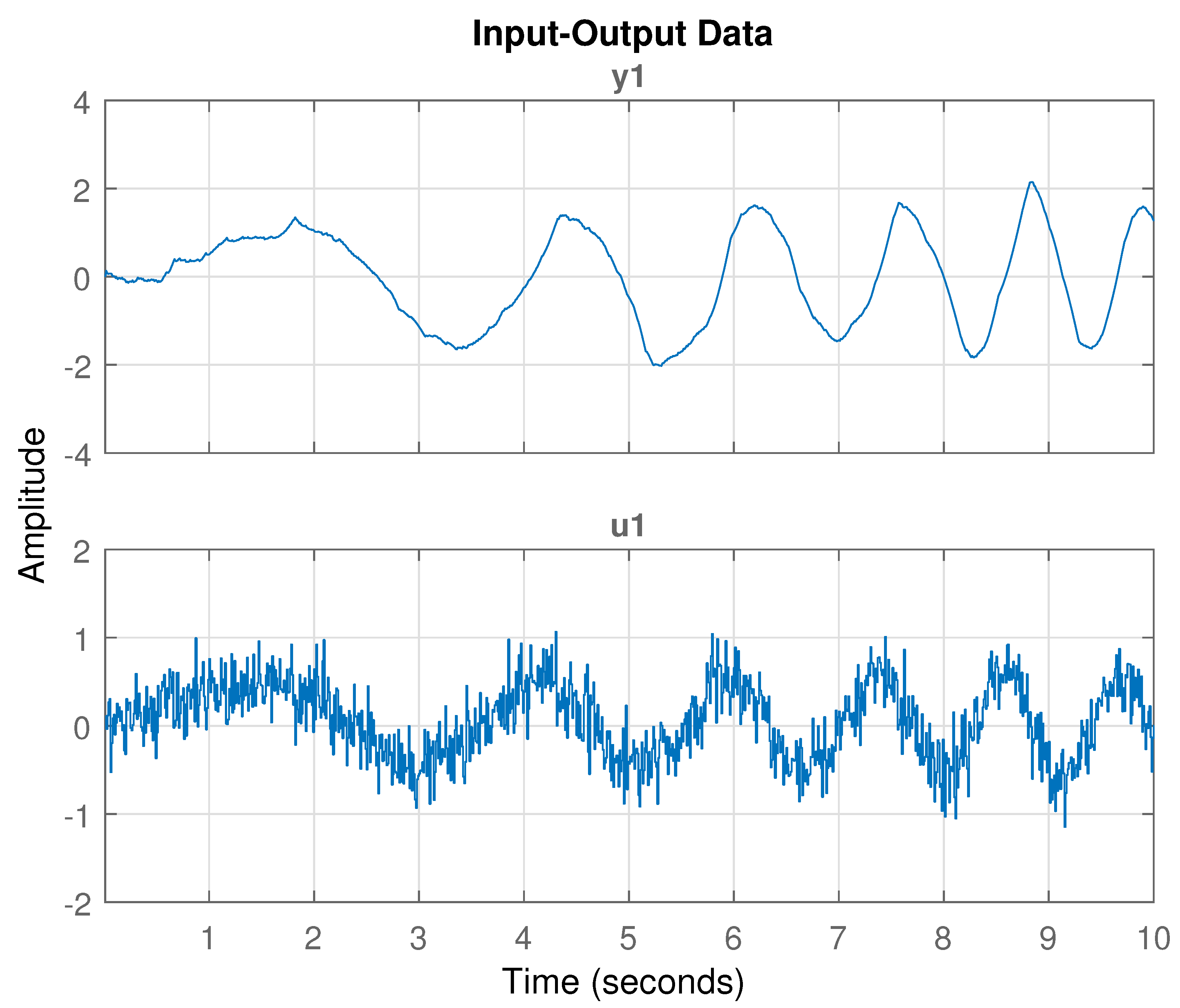
The structure of the data-set used in identification is determined by the type and parameters of the input excitation signal during the experiment. A commonly used input type when there is little or no a priori information about dynamic system is the frequency sweep [17], which is a continuous sinusoidal signal with increasing with time frequency in required band $\left[{\omega }_0,{\omega }_1\right]$ defined as $u\left(t\right)=sin({\omega }_{0}t+0.5({\omega }_1-{\omega }_0)t^2/T)+\eta \left(t\right)$, where T is the duration of the experiment. Models identified from frequency sweeps typically have good prediction capability and they are often applied in identification of hydraulically actuated aircraft during flight [18]. The application of such signal to the nonlinear model of the electro-hydraulic transducer and the recorded output response is presented on the Figure 3. Sample time for measuring the data and for the following models is $T_S=0.01s$ and the highest frequency from the sweep ${\omega }_1<2\pi /T_S$. Furthermore, a Gaussian random signal $\eta \left(t\right)$ is additively inserted in the excitation signal in order to account for the frequencies in the range $\left[{\omega }_1,2\pi /T_S\right]$.

The data from the Figure 3 are used only to calculate the estimates of the model parameters. A separate validation data-set is used to assess the quality of the estimated model through various test. The excitation signal for the validation is defined by generating another independent sample from the additive noise $\eta \left(t\right)$. After comparison of data-set to various possible model structures Box–Jenkins structure is selected as appropriate which fully decouples G and H transfer functions according to

$$y\left(z\right)=\frac{B\left(z^{-1}\right)}{F\left(z^{-1}\right)}u\left(z\right)+\frac{C\left(z^{-1}\right)}{D\left(z^{-1}\right)}e\left(z\right),$$

(4)

where $z=e^{j\omega T_S}$ and the polynomial $B\left(z^{-1}\right)={\sum }_{i=1}^8{b}_i{z}^{-1}$, $F\left(z^{-1}\right)=1-{\sum }_{i=1}^8{f}_i{z}^{-1}$, $C\left(z^{-1}\right)=1-{\sum }_{i=1}^2{c}_i{z}^{-1}$ and $D\left(z^{-1}\right)=1-{\sum }_{i=1}^8{d}_i{z}^{-1}$. The orders of the polynomials are chosen to minimize the variance of the parameter estimates, to achieve maximal fit to the data-set and to minimize the correlation $E\left[e\left(t\right)e(t-\tau )\right]$. Parameters $\theta ={(b_1,\dots ,b_8,c_1,c_2,d_1,\dots ,d_8,f_1,\dots ,f_8)}^T$, are estimated with prediction error method with initial conditions defined from previously estimated initial auto regressive model. The structure of the initial autoregressive model is selected from a set of other 1000 autoregressive models with various structure parameters according to the Akaike information criterion. Therefore the initial Box–Jenkins model used in estimation is corresponding to the initial auto regressive model in the following way

$$y\left(z\right)=\frac{{\sum }_{i=1}^8{b}_{i,init}{z}^{-i}}{1+{\sum }_{i=1}^8{a}_{i,init}{z}^{-i}}u\left(z\right)+\frac{1+{\sum }_{i=1}^2{c}_{i,init}{z}^{-i}}{1+{\sum }_{i=1}^8{a}_{i,init}{z}^{-i}}e\left(z\right),$$

(5)

where $b_{i,init}$ and $a_{i,init}$ are the coefficients of the numerator and the denominator polynomials from the initial autoregressive model. The prediction error method also calculates the covariance matrix $C_{\theta }=E\left(\theta {\theta }^T\right)$ which in turn is used in estimation of confidence ranges of the model frequency response. The estimated variance of the residual $E\left[e{\left(t\right)}^2\right]=1.8739\times {10}^{-4}$.

The comparison between the output of the linear Box–Jenkins model $y_m\left(t\right)$ and validation data-set $y\left(t\right)$ is in Figure 4, and the achieved level of fit is $J_{fit}=65.31\%$, where

$$J_{fit}=\frac{{\sum }_{k=0}^N{\left(y\left(k{T}_S\right)-y_m\left(k{T}_S\right)\right)}^2}{{\sum }_{k=0}^N{\left(y\left(k{T}_S\right)-{\sum }_{k=0}^{N}y\left(k{T}_S\right)\right)}^2}\times 100$$

(6)

When the comparison is with identification data-set which is used for calculation of parameter estimates the fit is higher $J_{fit}=73.45\%$ as expected. Residual correlation test for validation data set is presented in Figure 5 and indicates that parameter estimates are unbiased. Autocorrelation function of the signal $e\left(t\right)$ and the cross-correlation function between $e\left(t\right)$ and $u\left(t\right)$ are calculated with confidence level at $99\%$.

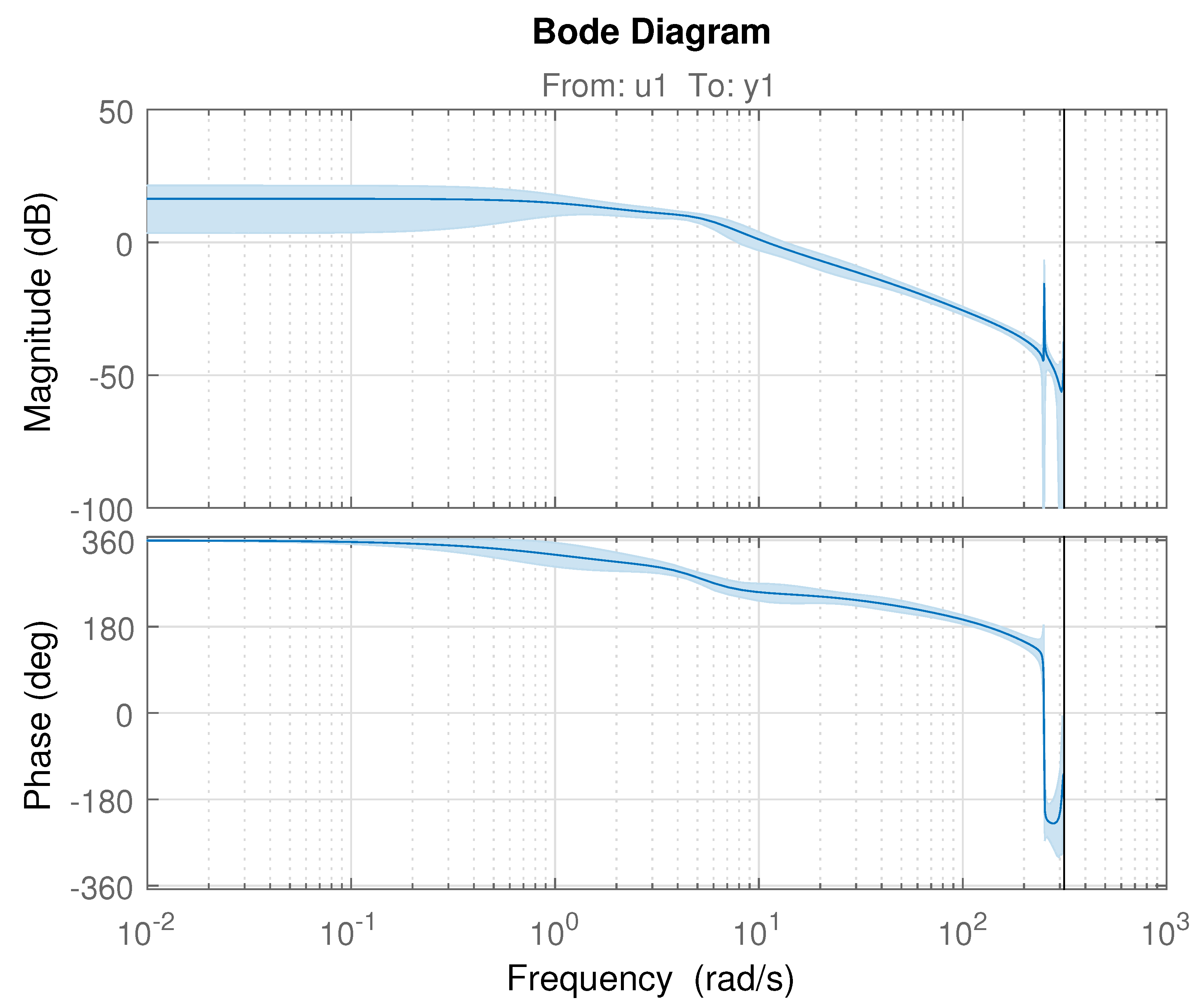
Covariance matrix of parameters $C_{\theta }$ contains the information about possible variations in the model parameters which as a consequence affects the frequency response of the model $G(j\omega ,\theta )$ and $H(j\omega ,\theta )$. As this dependence is explicit through the chosen model structure but nonlinear it can be simplified by employing Euler approximation formula in complex domain and to calculate standard deviation and confidence range of the frequency responses (Figure 6).

In accordance with Theorem 1 the confidence intervals for the $G(j\omega ,\theta )$ can define the multiplicative uncertainty filter $W_M\left(j\omega \right)$ in the model

$$G(j\omega ,\theta )=(1+W_M\left(j\omega \right)\mathsf{\Delta }(j\omega ,\theta ))G(j\omega ,E\left(\theta \right)),$$

(7)

where $∥\mathsf{\Delta }(j\omega ,\theta )∥\le 1$. However, to use $W_M\left(j\omega \right)$ for controller design it has to be parametrized as rational transfer function $B_M\left(j\omega \right)/A_M\left(j\omega \right)$

$$W_M\left(z\right)=\frac{{\sum }_{i=0}^7{b}_{i,m}{z}^{7-i}}{1+{\sum }_{i=0}^6{a}_{i,m}{z}^{6-i}}$$

(8)

Parametrization is calculated by fixing the order of numerator and denominator polynomials in $W_M\left(j\omega \right)$ and forming a system of linear equations for the magnitude response. This system has more equations than variable so the result is a solution in a least-squares sense. Figure 7 shows the correspondence between non-parametric and parametrized versions of $W_M\left(j\omega \right)$. The estimated noise variance for the initial auto regressive model is $E\left[e{\left(t\right)}^2\right]=2.1663\times {10}^{-4}$. The parametrization of $W_M\left(j\omega \right)$ allows to formalize the multiplicative uncertainty model in (7).

3. $\mathbf{\mu }$-Synthesis of Position Controller

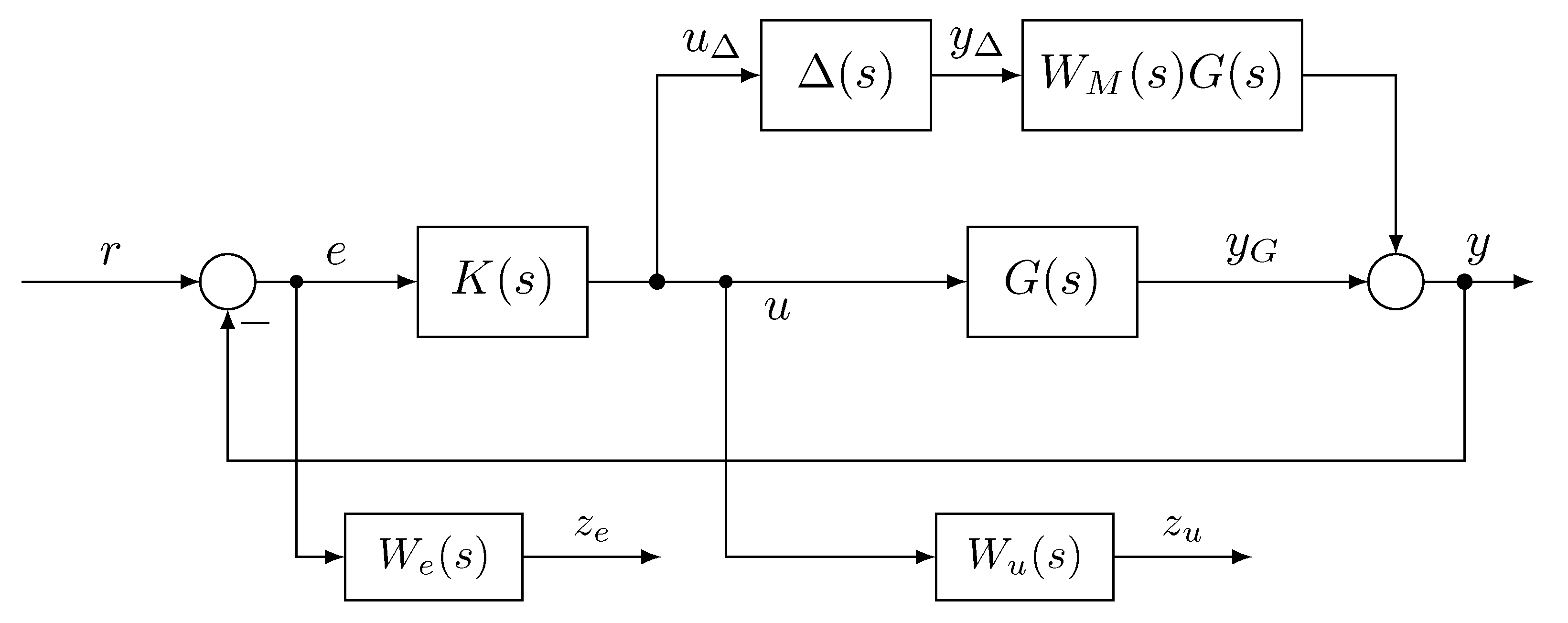
The aim of the $\mu$-regulator is to ensure robust stability and robust performance of spool position tracking in presence of unmodelled dynamics due to nonlinear part of the physical model. The closed-loop system for spool position control that includes the uncertain linear model, the controller and weighting functions reflecting the performance requirements is presented in Figure 8. The transfer function G is the nominal linear model of the electro-hydraulic transducer and $\mathsf{\Delta }$ is bounded uncertain transfer function. The controller output $u\in \left[-1,1\right]$ is the duty cycle of the pulse width modulated signals applied to the bridge of switching microvalves. The weighted closed-loop system outputs ($z_e$ and $z_u$) and the input to uncertain element ($u_{\mathsf{\Delta }}$) are related to the reference signal r and disturbance $y_{\mathsf{\Delta }}$ as

$$\left(\begin{array}{c}{u}_{\mathsf{\Delta }}\\ z_e\\ z_u\end{array}\right)=\left(\begin{array}{cc}KS{W}_{M}G& KS\\ -W_{S}S{W}_{M}G& W_{e}S\\ W_{u}KS{W}_{M}G& W_{u}KS\end{array}\right)\left(\begin{array}{c}{y}_{\mathsf{\Delta }}\\ r\end{array}\right)$$

(9)

where $S={(I+GK)}^{-1}$ is the output sensitivity function and $KS$ is the input sensitivity function.

The $\mu$-synthesis is based on iterative $H_{\infty }$ optimization which is easy to solve in continuous time when $D_{12}\ne 0$ and $D_{21}\ne 0$. As the resultant uncertain linear time invariant model is represented in discrete time and the following developments of the $\mu$-controller is in continuous time the plant model is approximated by using the inverse Tustin formula $z\mapsto \frac{1+s{T}_S/2}{1-s{T}_S/2}$.

The control problem is to select a regulator $K\left(s\right)$ such that transfer function from the exogenous input signal r to the output signals $z_e$ and $z_u$ to be small in the sense of H-infinity norm for all possible uncertain plant models represented with $\mathsf{\Delta }$. The transfer functions $W_e$ and $W_u$ express the relative importance of the performance in the various frequency ranges. The output sensitivity weighting $W_e\left(s\right)=\frac{1000}{(40s+1)(0.1s+1)}$ is selected such that low frequency errors to be minimized and closed-loop bandwidth to be at $0.025s^{-1}$. Further, after $10s^{-1}$ weight is further relaxed as such frequencies are beyond switching period of the micro valves. The input sensitivity weighting $W_u\left(s\right)=1.1\frac{0.02s+1}{0.2s+1}$ is tuned to keep the manipulated variable u in its predefined bounds and in its effective frequency range of action. Too fast rates of u cannot be accepted by the physical model again due to switching nature of actuation. The closed-loop system should remain stable for all ${∥\mathsf{\Delta }∥}_{\infty }<1$ and in addition the performance criteria

$${∥\left(\begin{array}{c}{W}_{e}S\\ W_{u}KS\end{array}\right)∥}_{\infty }<1$$

(10)

to be satisfied too. Let us define the uncertain matrix ${\mathsf{\Delta }}_{perf}=\left(\begin{array}{ccc}\mathsf{\Delta }& 0& 0\\ 0& {\mathsf{\Delta }}_e& 0\end{array}\right)$. The first block of the matrix ${\mathsf{\Delta }}_{perf}$ corresponds to the input multiplicative uncertainty from the physical model. The second and the third blocks—${\mathsf{\Delta }}_e$ is a fictitious uncertainty block used to include the performance requirements into the $\mu$-synthesis framework. The input to this block is the weighted tracking error signal $z_e$ and the output is the reference signal r. The aim of the $\mu$-synthesis is to find a stabilizing controller $K\left(s\right)$ such that at each frequency $\left[0,\pi T_S\right]$ the structured singular value satisfies the condition

$${\mu }_{{\mathsf{\Delta }}_{perf}}\left(\left[\begin{array}{cc}KS{W}_{M}G& KS\\ -W_{S}S{W}_{M}G& W_{e}S\\ W_{u}KS{W}_{M}G& W_{u}KS\end{array}\right]\right)<1$$

(11)

which guarantees that performance requirement (10) for the closed-loop too. The minimization is achieved by an approximate procedure—so-called D-K Iteration based on the upper bound ${\mu }_{\mathsf{\Delta }}\left(M\right)<{∥D_{L}M{D}_R∥}_{\infty }$, where $D_L$ and $D_R$ are minimum phase scaling matrices and M is the lower fractional transform of the controlled plant [19]. Therefore, the following suboptimal problem is solved for each $\omega$

$$\underset{K}{min}\underset{D_L,D_R\in {\mathcal{H}}_{\infty }}{inf}{∥D_{L}M{D}_R∥}_{\infty }$$

(12)

The magnitude frequency response of the synthesized $\mu$-controller (Figure 9) indicates an integrating effect in the low frequency range which is necessary for reference trajectory tracking. The achieved $\mu$ value of 0.974 means that the uncertain system can tolerate all of the modeled uncertainty. The controller is from 28th order.

Sensitivity functions of the closed-loop system with the controller and for various randomly taken values for the uncertain element are presented in Figure 10 and Figure 11. On the figures are also shown the inverses of the weighting functions $W_e$ and $W_u$, which specify the performance requirements for the loop. As can be seen the disturbance attenuation at low frequency is about 1000 times and the closed-loop keep its prescribed performance in presence of uncertainty.

Figure 11 shows the influence of the references and disturbances on the control action. In high frequency range the measurement noise is slightly amplified. Depending on position sensor characteristics the noise influence on the control may be decreased at the expense of smaller disturbance attenuation.

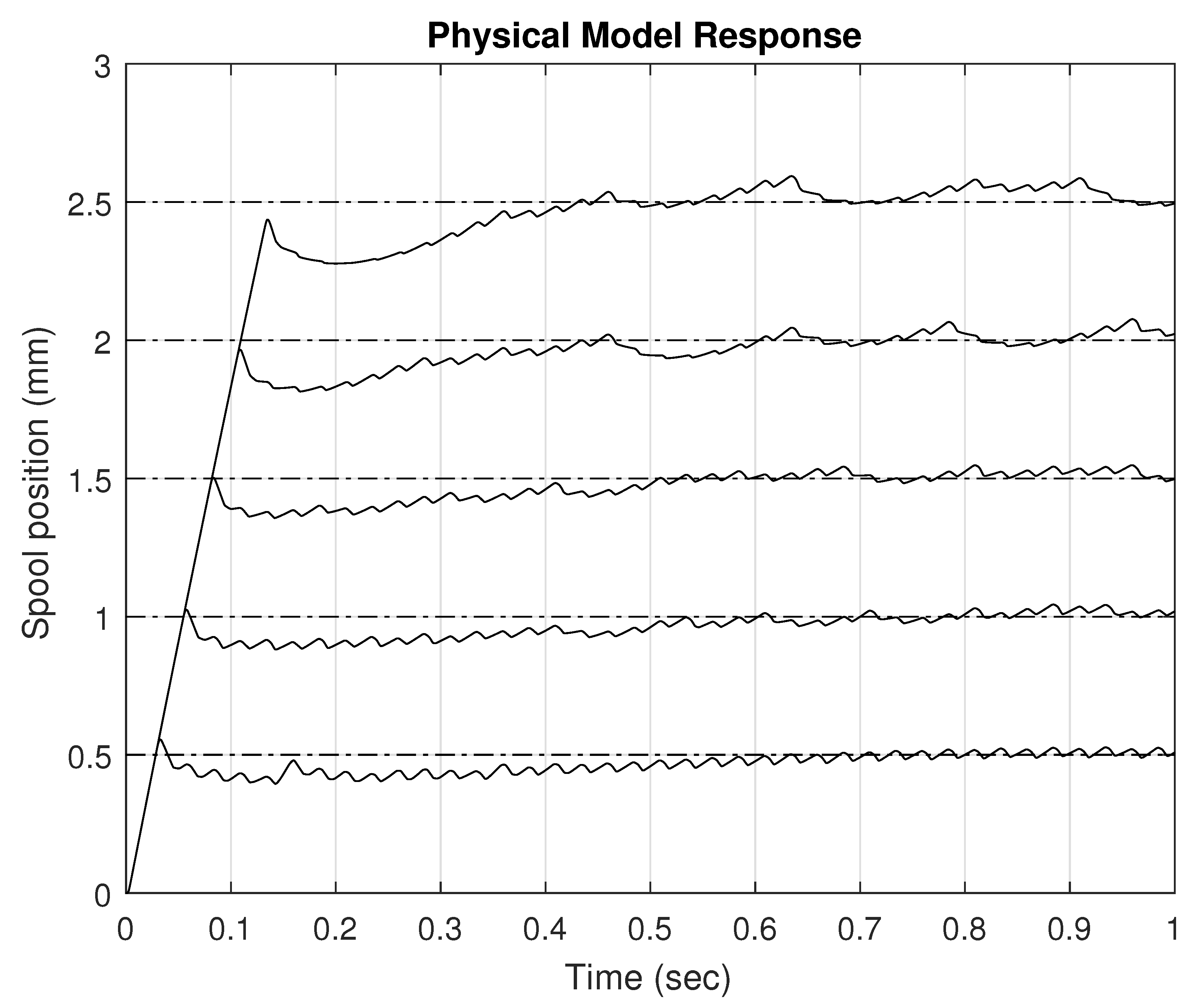
To further investigate the performance of the controller it is tested with the nonlinear physical model of the electro-hydraulic actuator. There the model parameters are fixed but the plant model is nonlinear and the control action is constrained $u\in \left[-1,1\right]$. These results are presented in Figure 12 for step reference signal and in Figure 13 for band-limited reference signal. During the step reference signal there is overshot in the position response which is increasing with the amplitude of the reference—for $0.5$ mm the overshot is $0\%$ but for $2.5$ mm it is almost $20\%$. Obviously this is due to the nonlinearity in the system and look like a wind-up effect. Therefore, we make the following assumption.

Assumption 1.

The cause for the overshot in the step response of the nonlinear closed-loop system with the linear μ-controller is the saturation of the control signal u.

For now the supporting argument for such a claim is apparent integral nature of the controller (Figure 9) and the observed saturation of the control action during the rising period of the output signal (Figure 14). In addition, if the reference trajectory is with limited bandwidth, such as in Figure 13, then the overshot disappears. The remaining oscillation comes from high-frequency switching of the micro valves and cannot be compensated.

4. Controller Modification for Anti Wind-Up

In order to attenuate observed wind-up effect we decided to exploit the structure of the $\mu$-controller by explicitly introducing the saturated control action. For the following analysis $u_{sat}\in \left[-1,1\right]$ denote the saturated control, and $u=K(r-y)$ denote the unsaturated output of the controller K. Furthermore, $\xi =u_{sat}-u$ denote an input disturbance signal. The input to the linear plant model becomes $u_{sat}=u+\xi$. The aim here is to construct a modified controller $K_{mod}\left(s\right)$ which calculates a control action $u_{mod}$ as

$$u_{mod}=K_{mod}\left(s\right)\left(\begin{array}{c}{u}_{sat}\\ r-y\end{array}\right),$$

(13)

such that $u_{mod}\left(t\right)=u\left(t\right)$ if and only if $u\left(t\right)=u_{sat}\left(t\right)$, $\forall t>T_{sat}$, where $T_{sat}>0$ is the duration of the saturation period.

According to (12) the $\mu$-controller can be regarded as a $H_{\infty }$-controller for a scaled plant $D_{L}M{D}_R$

$$D_{L}M{D}_R=\left(\begin{array}{ccc}A& B_1& B_2\\ C_1& D_{11}& D_{12}\\ C_2& D_{21}& D_{22}\end{array}\right)$$

(14)

and the matrix D in our case is

$$D=\left(\begin{array}{ccc}0& 0& 0.01358\\ -3\times {10}^{-4}& -1\times {10}^{-4}& {10}^{-6}\\ 0& 0& 0.08526\\ 2.941& 1& 0.01375\end{array}\right)$$

(15)

and assume that $D_{11}\approx 0$. It has been verified that such a change does not account for any significant effect in the controller frequency response or closed-loop dynamics. However, it simplifies the analytic form of the controller. The controller K is calculated from the solution of the Riccati equations corresponding to the controllability and the observability Hamiltonians. The bound for $\gamma =0.974$ is fixed according to

Table 1. A summary of the DK-iterative procedure.

Iteration	1	2	3	4	5
Controller Order	24	28	28	28	28
D-Scale Order	6	10	10	10	10
Achieved $\gamma$	2.309	1.043	0.974	0.977	0.981
Peak $\mu$	2.192	1.038	0.974	0.977	0.981

such that ${∥D_{L}M{D}_R∥}_{\infty }<\gamma$.

Then, the regulator takes the form

$$K\left(s\right)=\left(\begin{array}{cc}{A}_K& -H_2{r}_{21}\\ r_{12}{F}_2{Z}_{\infty }& 0\end{array}\right)$$

(16)

where $r_{12}$ and $r_{21}$ are from singular value decomposition of the matrices $D_{12}$ and $D_{21}$ in order for their normalization to a standard form, $Z_{\infty }$ is the product of the solutions of the controllability and observability Riccati equations, H is the observer gain partitioned as

$$p=\left(\begin{array}{ccc}{H}_{11}& H_{12}& H_2\end{array}\right)\left(\begin{array}{c}\left(\begin{array}{c}{u}_{\mathsf{\Delta }}\\ z_e\end{array}\right)\\ z_u\\ y\end{array}\right)$$

(17)

The state feedback gain F is partitioned as

$$\left(\begin{array}{c}{y}_{\mathsf{\Delta }}\\ r\\ u\end{array}\right)=\left(\begin{array}{c}{F}_{11}\\ F_{12}\\ F_2\end{array}\right)p$$

(18)

Here, $p\left(t\right)$ is a vector of internal state variables of the controller $K\left(s\right)$. The matrix $A_K$ for the the case of $D_{11}=0$ is

$$\begin{array}{c}{A}_K=A+HC+{\widehat{B}}_2{\widehat{C}}_1-\tilde{B}\left((I-M){\tilde{D}}^{-1}\right)\tilde{C}=\hfill \\ A+HC+(B_2+H_{12}-m{r}_{21}{H}_2)F_2{Z}_{\infty },\hfill \end{array}$$

(19)

where ${\widehat{B}}_2=B_2+H_{12}$, ${\widehat{C}}_1=F_2{Z}_{\infty }$,

$$\tilde{B}=\left(\begin{array}{cc}-H_2{r}_{21}& {\widehat{B}}_2\end{array}\right),\tilde{C}=\left(\begin{array}{c}{r}_{12}{F}_2{Z}_{\infty }\\ -(C_2+F_{12})Z_{\infty }\end{array}\right),$$

(20)

$M={(I+{\tilde{D}}_{22}\tilde{D})}^{-1}=\left(\begin{array}{cc}1& m\\ 0& 1\end{array}\right)$ is a term related to the value of $D_{22}\ne 0$, where

$$\tilde{D}=\left(\begin{array}{cc}0& r_{12}\\ r_{21}& 0\end{array}\right),{\tilde{D}}_{22}=\left(\begin{array}{cc}0.01375& 0\\ 0& 0\end{array}\right)$$

(21)

Let us examine the matrix $A_K$ defined with (19), and noting that $u=C_{k}p=r_{12}{F}_2{Z}_{\infty }$, we can possibly substitute the term $F_2{Z}_{\infty }$ with $u_{sat}/r_{12}$ in order to introduce some information about control saturation into controller. The following theorem gives conditions about when such a substitution would lead to attenuation of the input disturbance $\xi$.

Theorem 2.

Let the controller $K\left(s\right)$ is of the form (16) and $(\exists M)(A_K={\overline{A}}_K+M{C}_K)$. Moreover, let the controller $K_{mod}\left(s\right)$ is defined by the substitution $C_{K}p\left(t\right)\mapsto u_{sat}\left(t\right)$. Then, $\left|\right|u_{mod}{\left|\right|}_2{<\left|\right|u\left|\right|}_2$ for every $r\in {\mathcal{L}}_2$ if $\left(B_K^T{B}_K\right)B_K^{T}M>0$.

Proof. 

In Appendix A. □

The expression (19) for the matrix $A_K$ offers seven choices for the matrix M which are summarized in the

Table 2. Selection of the anti wind-up gain.

Choice for ${\mathit{r}}_{12}\mathit{M}$	$\mathit{max}\left(\mathit{Re}\mathit{\lambda }({\mathit{A}}_{\mathit{K}}-{\mathit{C}}_{\mathit{K}}\mathit{M})\right)$	$\left({\mathit{B}}_{\mathit{K}}^{\mathit{T}}{\mathit{B}}_{\mathit{K}}\right){\mathit{B}}_{\mathit{K}}^{\mathit{T}}\mathit{M}$
$B_2+H_{12}-m{r}_{21}{H}_2$	$-0.025$	0.0043
$B_2+H_{12}$	$-1.1487$	0.0181
$H_{12}-m{r}_{21}{H}_2$	$0.1608$	−0.0137
$B_2-m{r}_{21}{H}_2$	$-0.025$	0.0043
$B_2$	$-1.1487$	0.0181
$H_{12}$	$-0.025$	$4\times {10}^{-20}$
$-m{r}_{21}{H}_2$	$0.1608$	−0.0137
0	$-0.025$	0

. It can be observed that they lead to various damping rates which are characterized by the minimal real part of the eigenvalues of the matrix $A_K-C_{K}M$. Two of the choices would make the closed-loop even unstable. Therefore, in order to achieve the faster convergence we have selected $M=B_2+H_{12}$.

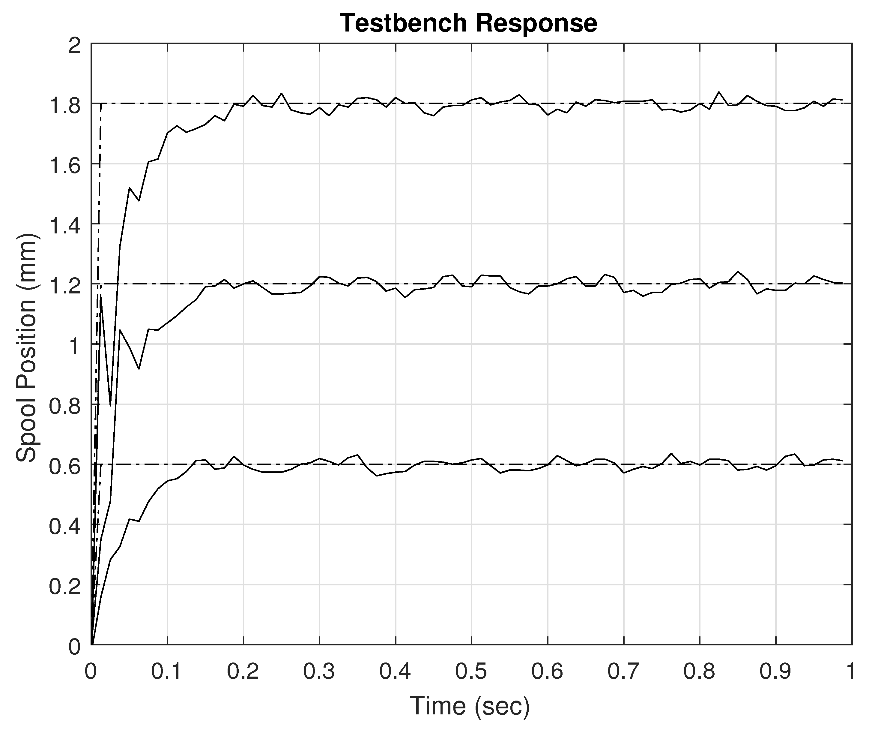
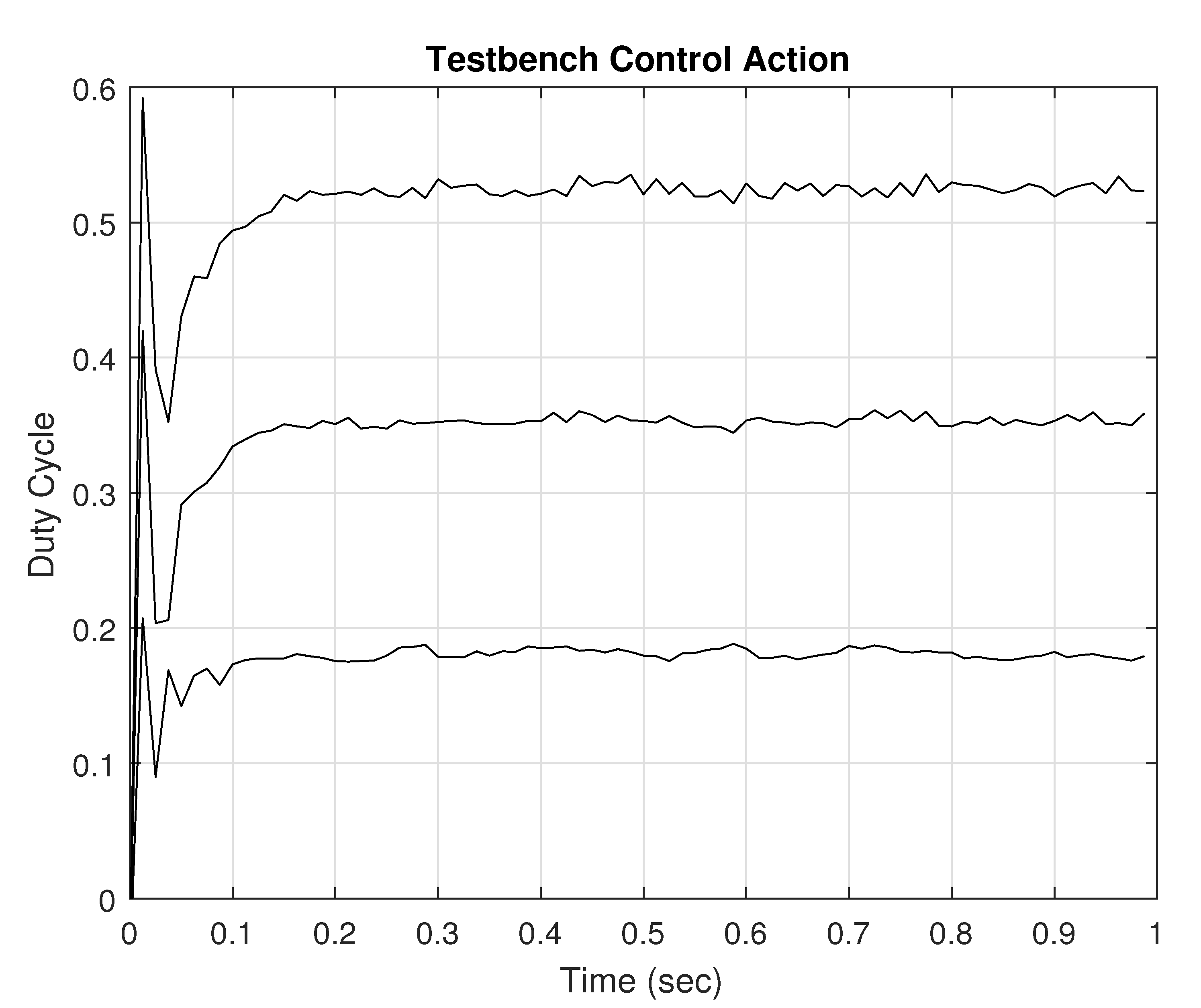
The controller is then applied to the nonlinear physical model. The results for spool position responses are presented in Figure 15 and the corresponding control actions are in the Figure 14. The modified controller successfully attenuates the wind-up effects observed on the Figure 12.

5. Experimental Results

We have constructed a laboratory hydraulic test equipment for an electro-hydraulic steering unit with load-sensing RM technology (OSPEC200), complying with the current electro-hydraulic power steering systems requirements. The implemented test rig layout includes a MC012-022 microcontroller, a programmable joystic (JS6000) for supplying operator commands, and the spool valve, pilot operated with switching micro valves, which drives a hydraulic servo cylinder. The position of the cylinder piston is obtained with the resistive position sensor. The $\mu$-controller algorithm, which is originally designed as a Simulink model is translated to structured text language (according to IEC 61131-3) by employing automatic code generation through the Simulink PLC Coder.

Figure 16 shows a picture of the laboratory test bench with its main components highlighted. Figure 17 presents the measured spool position step response for various amplitudes, and in Figure 18 is the corresponding control signal.

6. Conclusions

The main contribution of the article is successful design and application of a high-order robust controller to control the position of a spool valve through switching digital valves. The implemented $\mu$-controller guarantees robust stability and robust performance analyzed through examination of the structured singular value of the uncertain closed-loop system. The robust performance practically means that system will keep its tracking accuracy even in presence of relatively large parameter variations or strong external disturbances.

Another contribution is in the propose anti-windup modification of the standard $\mu$-controller. In addition, such an approach can be used to control of other electro-hydraulic drive systems with complex dynamics. The classical approach for such situations is optimal selection of anti-windup compensator $R\left(s\right)$. However, we investigate an alternative approach which modifies the internal structure of the controller. In future investigation, we will try to connect the proposed approach in the unified coprime-factorization framework as in the works of Morari. Alternatively, the use of a pre-filter on the reference signal may improve the tracking performance of the closed-loop system but it should be tuned with respect to some optimization criteria as well. Results before and after the anti wind-up scheme are presented when the nonlinear simulation model is utilized. However the controller without anti-windup modification is not tested experimentally because a large overshoot at the end of spool range may cause some mechanical damage.

A critical component for the successful design and implementation of the robust embedded controller is the availability of an accurate linearized dynamical model of the controlled system. From the nonlinear analytic model of the hydraulic spool valve we know that the nonlinearity is mainly in the the low frequency range and can be represented by smooth functions. Another nonlinearity in the high frequencies is the discontinuity due to switching behavior. Determining a model-parameter subset with “high probability” from the covariance matrix can be questioned for the nonlinear models because such covariance matrix lies on the assumption of normally-distributed white-noise disturbance input and model being “in the model class”. However, it is clear that switching dynamics of the micro valve bridge can be equivalently represented in the model by its averaged pressure–flow characteristic acting upon the spool. The other nonlinear terms in the analytical model are monotone (products, squares, powers) and not periodic functions. The whole system is constructed by design to behave as a monotone or linear-like, meaning that an increase in the input variable will lead to a proportional as a scale increase in the output variable. That is because the spool response has to mimic a steering wheel if a human operator directly manipulates it. Therefore, the role of the nonlinearity in the model can be considered as a disturbance upon the valve response caused by an inherent properties of the fluid equations which cannot be compensated with the valve geometry design. Therefore, should exists a reasonable linear approximation $G\left(j\omega \right)$ to the system dynamics (obtained for example with Taylor linearization around the neutral valve position), of course coming with a respective output disturbance (higher Taylor series terms), which eventually will be accounted in the residual $e\left(k{T}_S\right)$. Thus, the model belonging to the model class is actually the Taylor approximation $G\left(j\omega \right)$, which is guaranteed to exist for the case of our model. The only problem here is how to choose the model class to make sure that $G\left(j\omega \right)$ will belong to it and the solution is to select a higher order of the model structure with independent noise dynamics (like the Box-Jenkins from the 8th order utilized in the article).

The assumption of normally-distributed white-noise disturbance $e\left(k\right)$ is a prerequisite for almost any statistical method. Moreover, if $e\left(k\right)$ is not normally-distributed or not white-noise then there exists a Gaussian approximation process $v\left(k\right)$ such that $E\left(v\right(k\left)\right)=E\left(e\right(k\left)\right)$ and $E\left(v2\right(k\left)\right)=E\left(e2\right(k\left)\right)$. The higher moments $E\left(en\right(k\left)\right)$, $n>2$, which describe the statistics of $e\left(k\right)$ will not be captured by the $v\left(k\right)$ but both signals will eventually span a same range of values which is practically acceptable for a random variable. In conclusion we will get more conservative results if we approximate a non-Gaussian process with a Gaussian one but the model will be still correct, despite conservative or with larger covariance of parameters.