
Calculation of the Shading Factors for Solar Modules with MATLAB


Abstract
:1. Introduction
2. The Shading Factors
2.1. Direct Irradiance Shading Factor
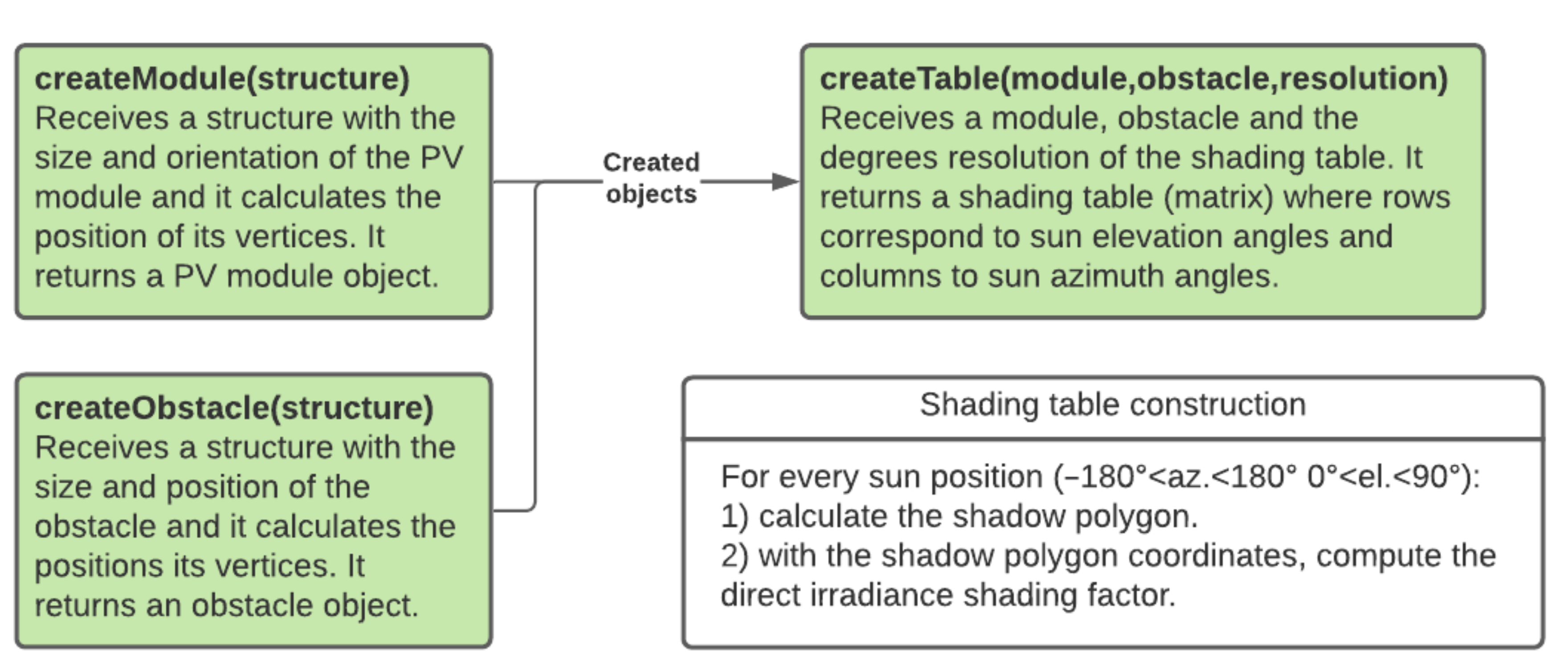
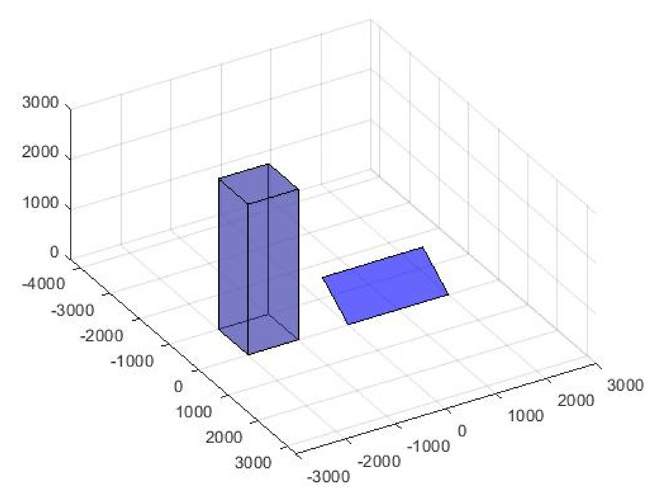
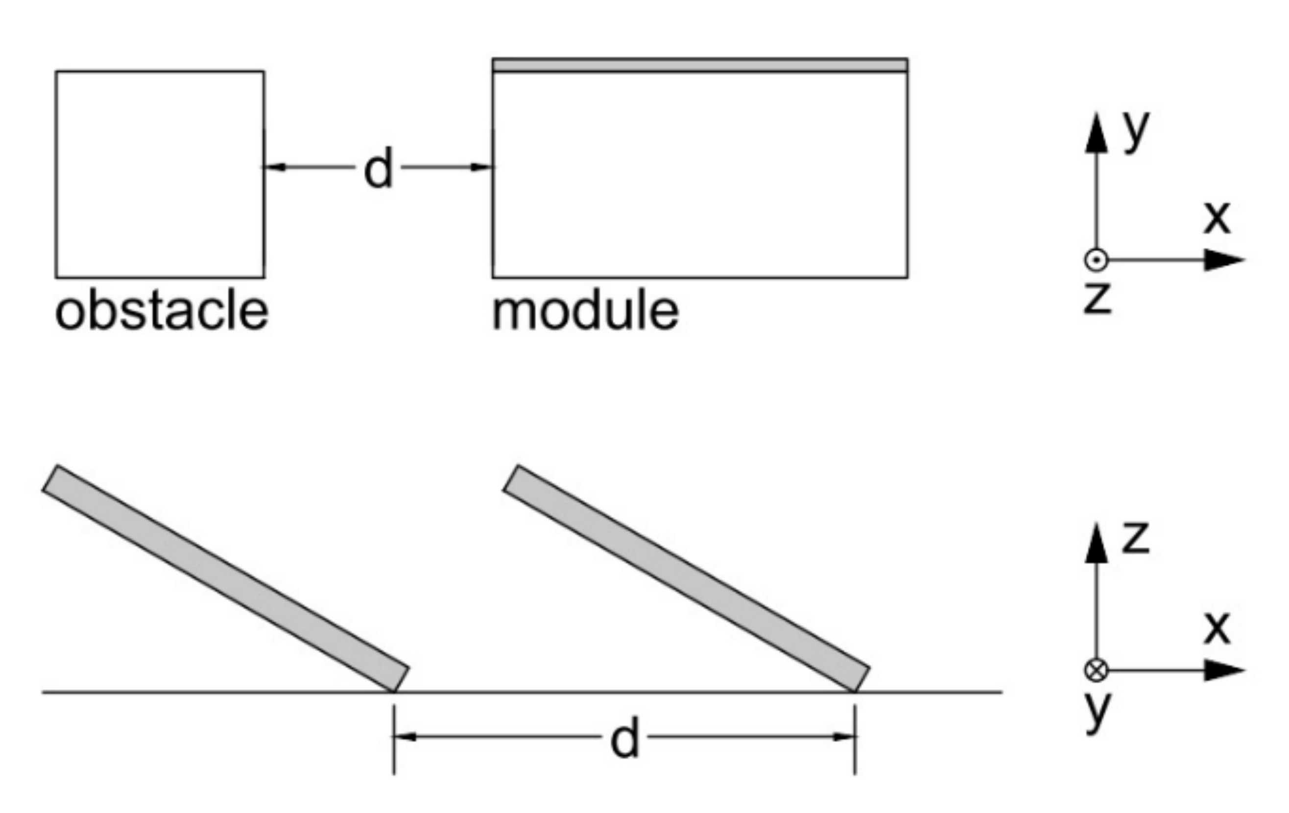
2.1.1. Module Geometry Definition
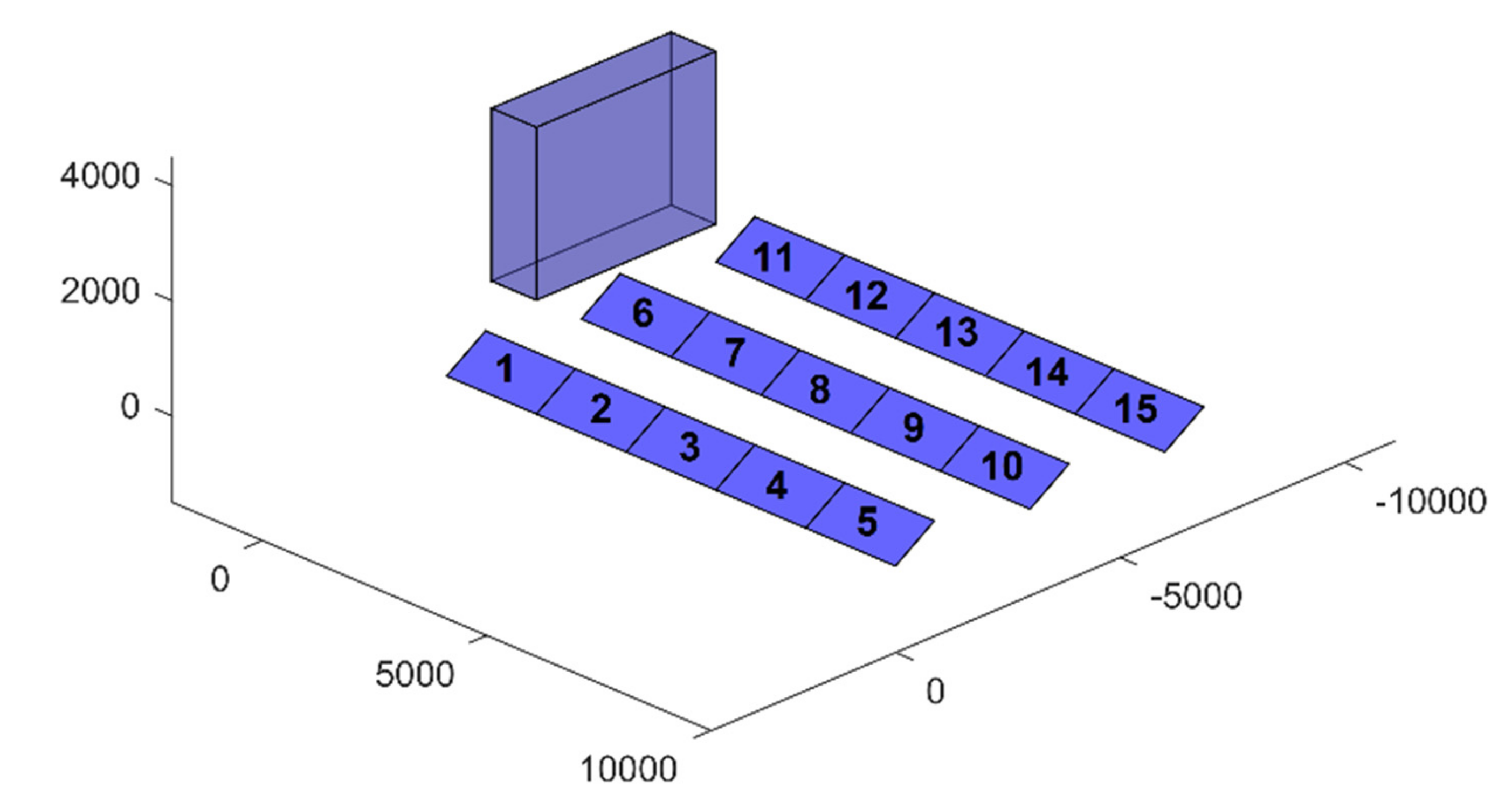
2.1.2. Obstacle Geometry Definition
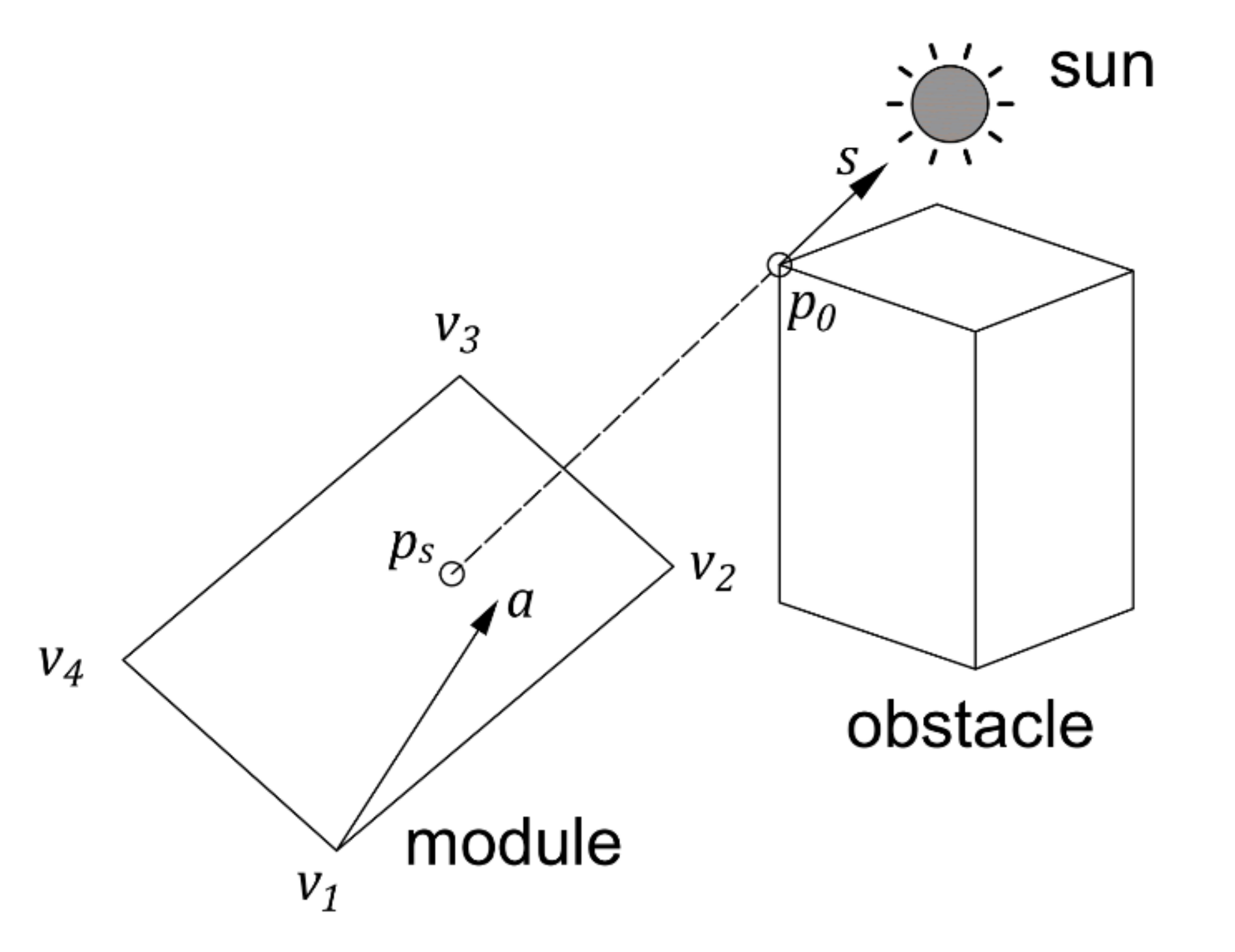
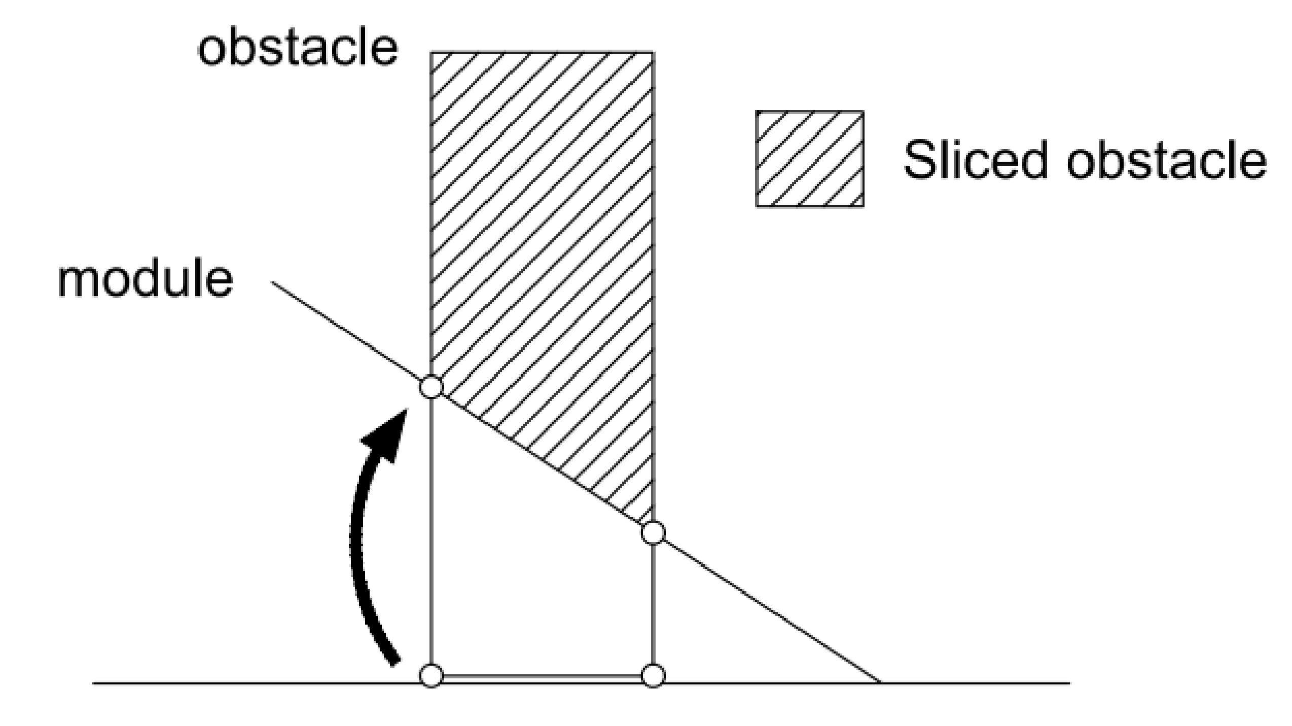
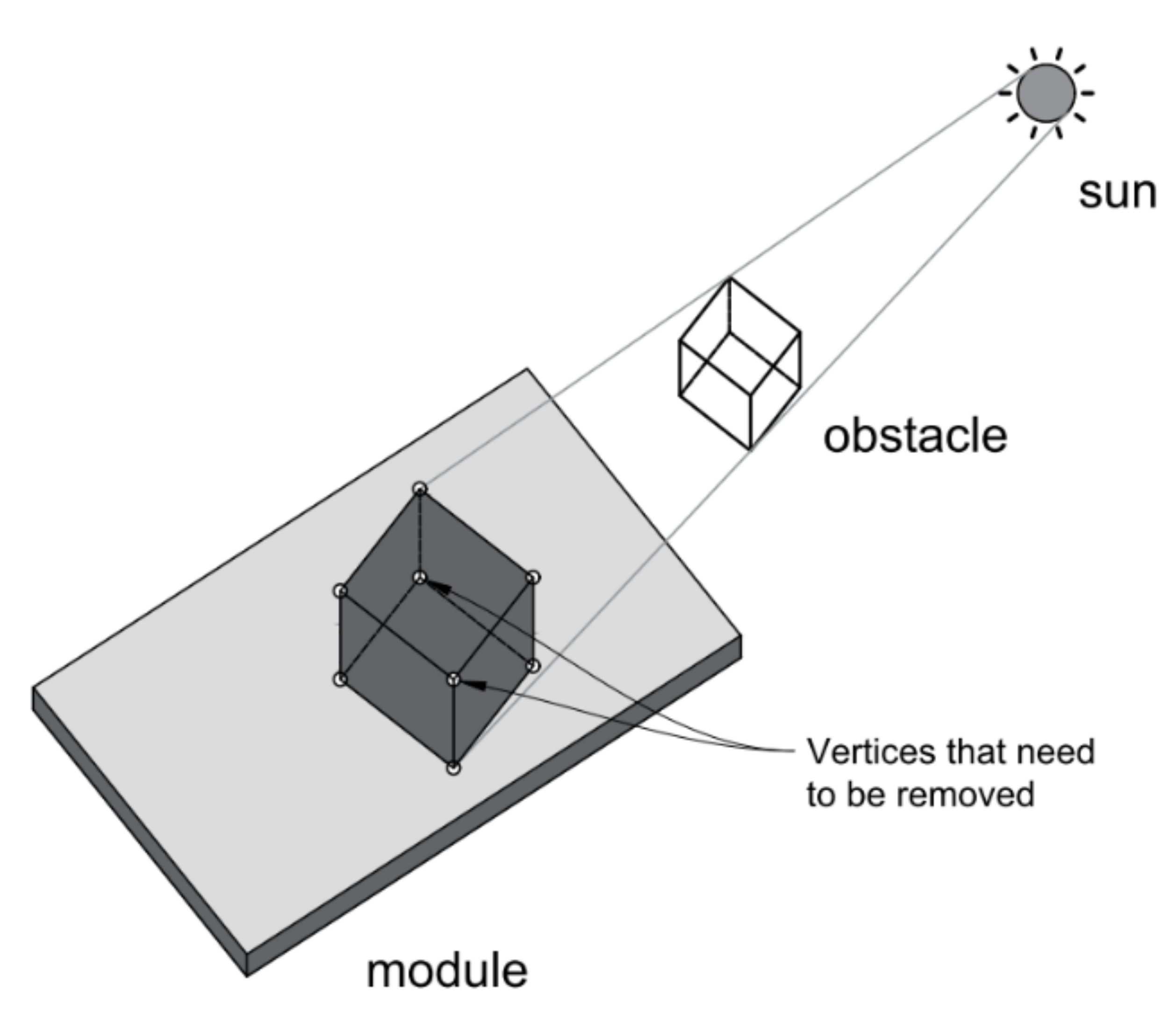
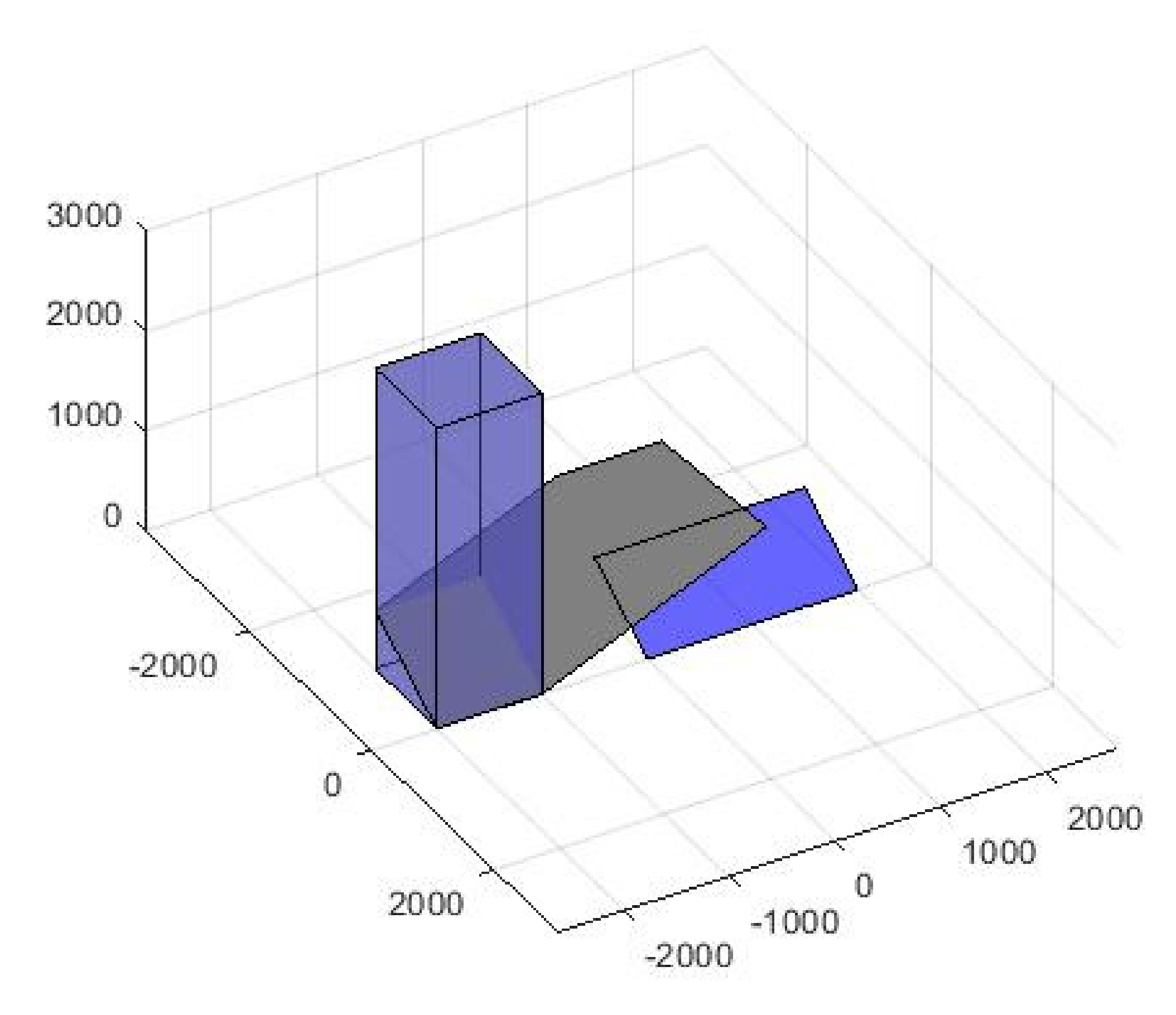
2.1.3. Shadow Calculation Procedure
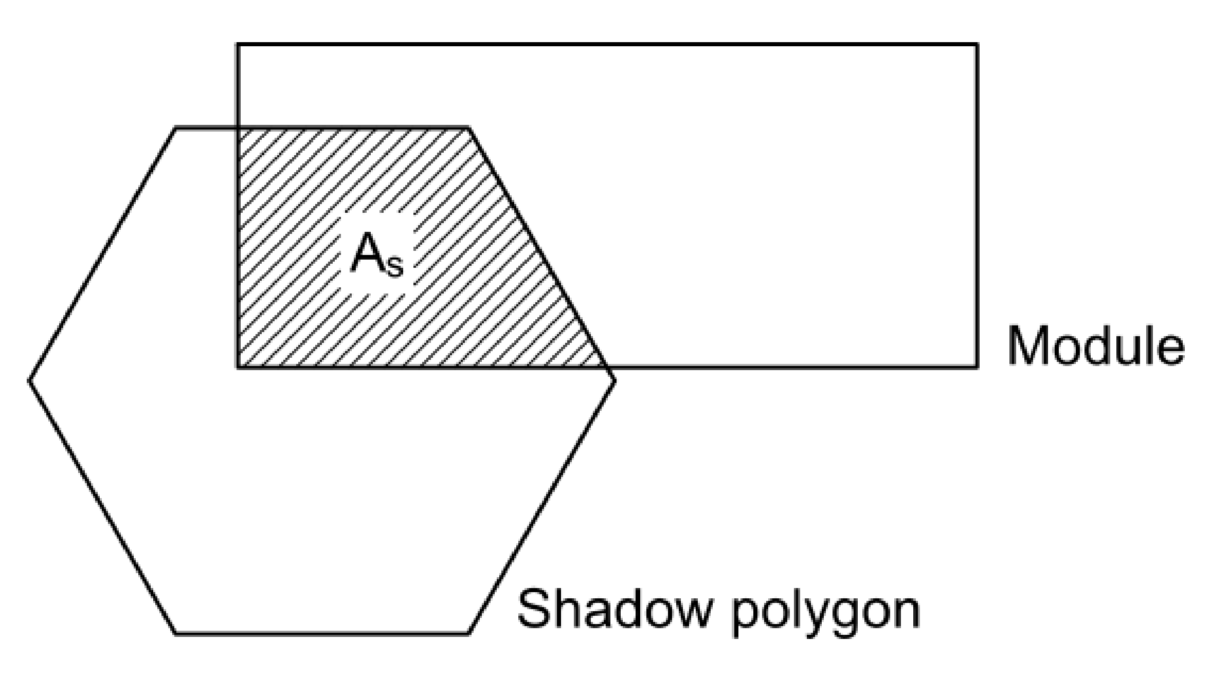
2.1.4. Shading Factor Calculation
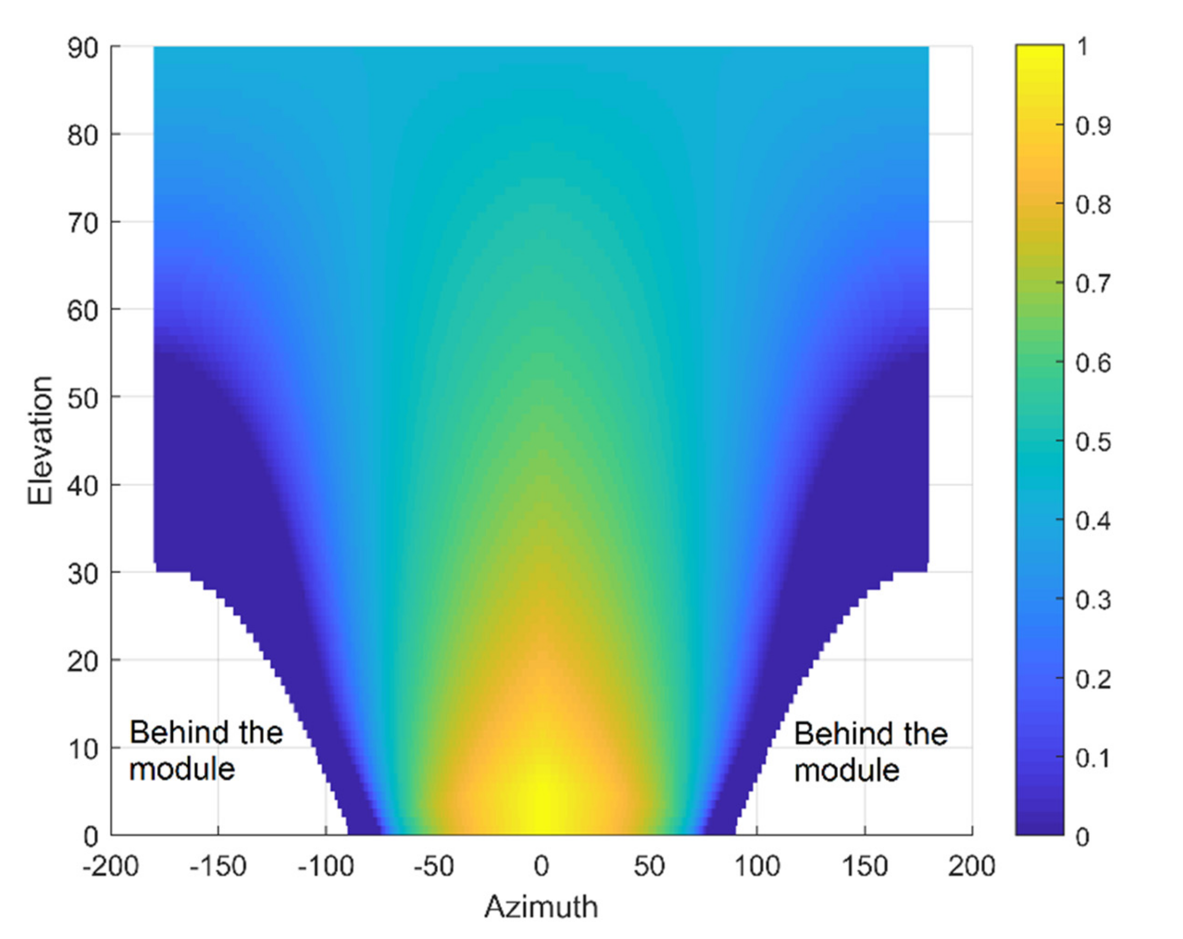
2.1.5. Shading Table
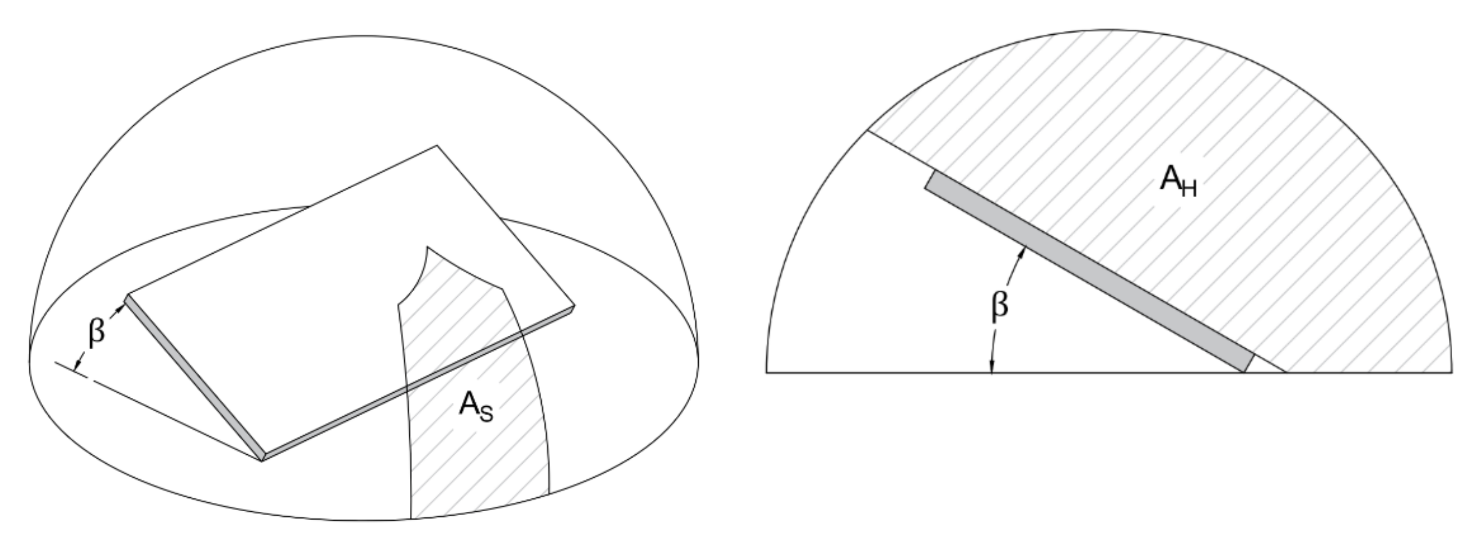
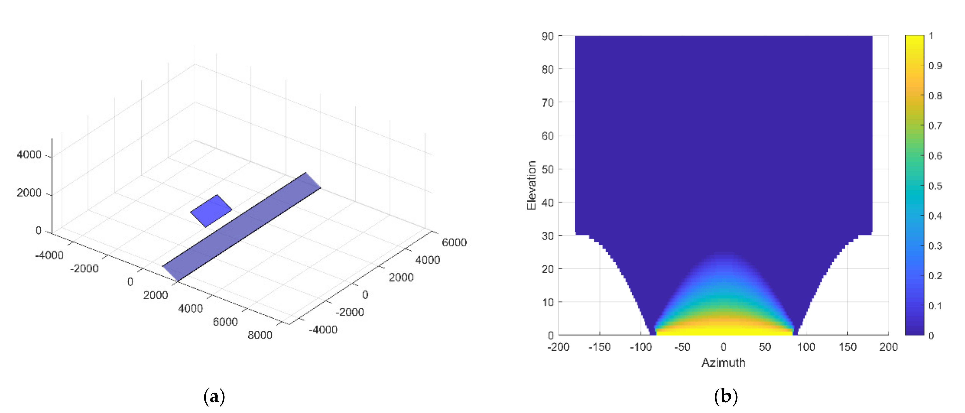
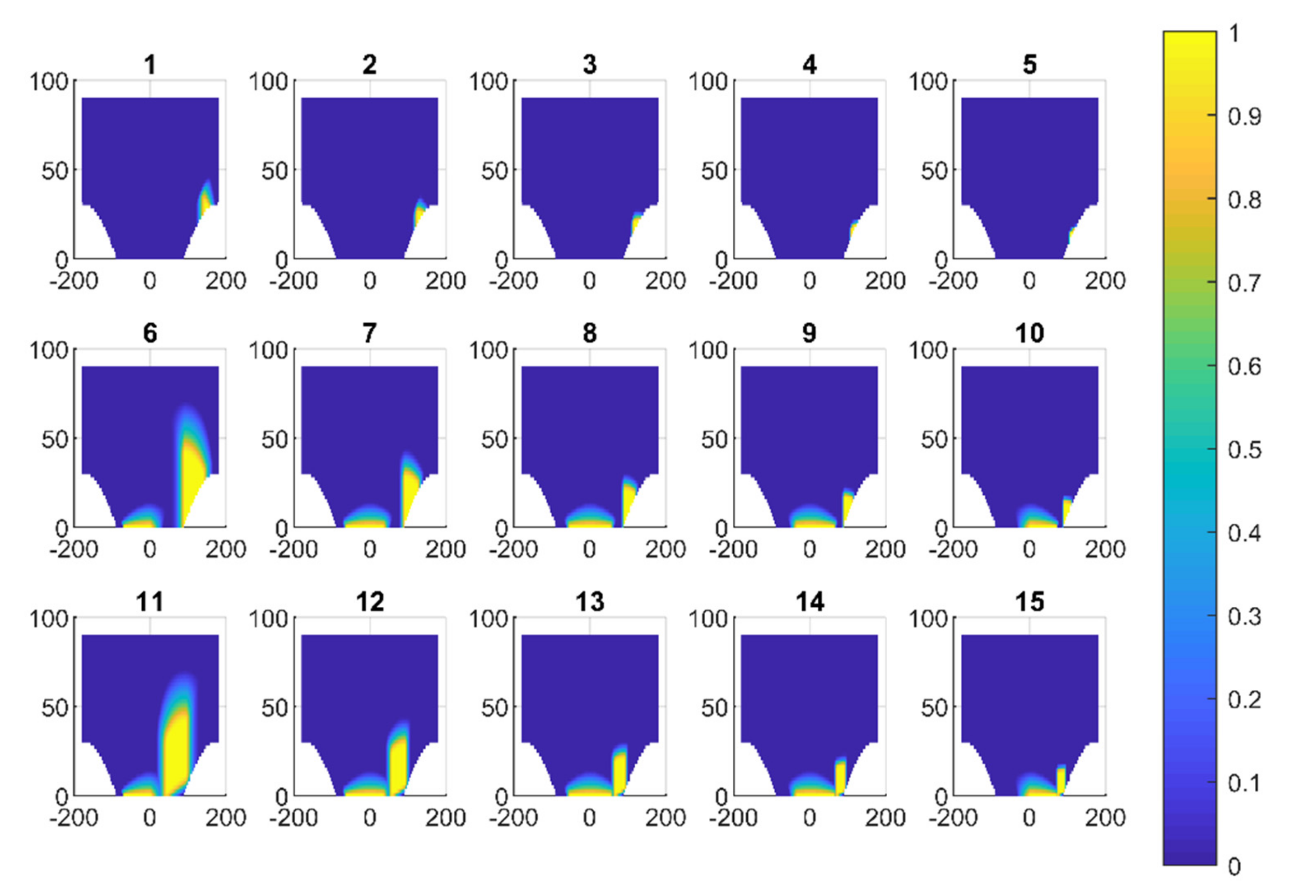
2.2. Diffuse Shading Factor
2.3. PV Array Class
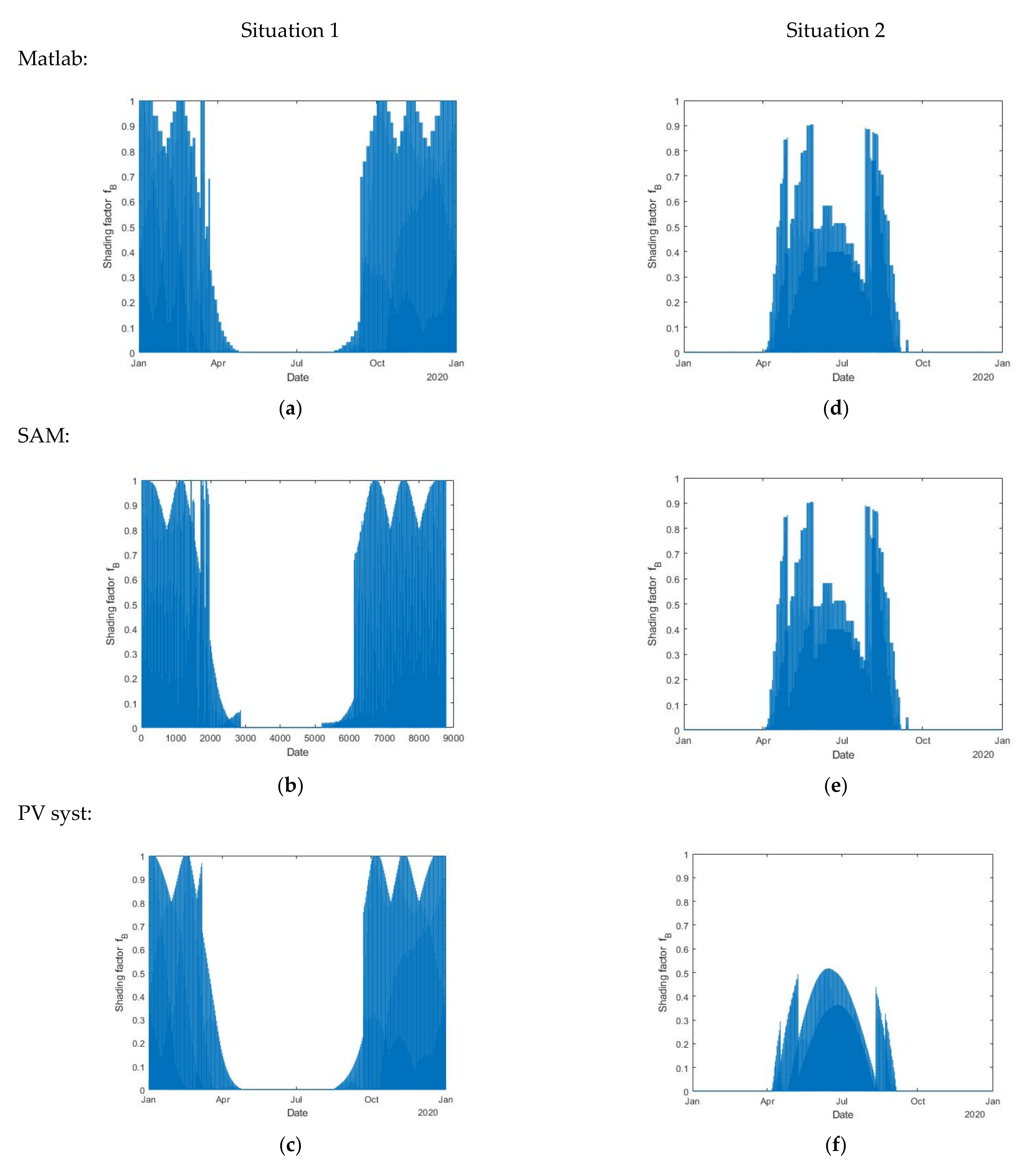
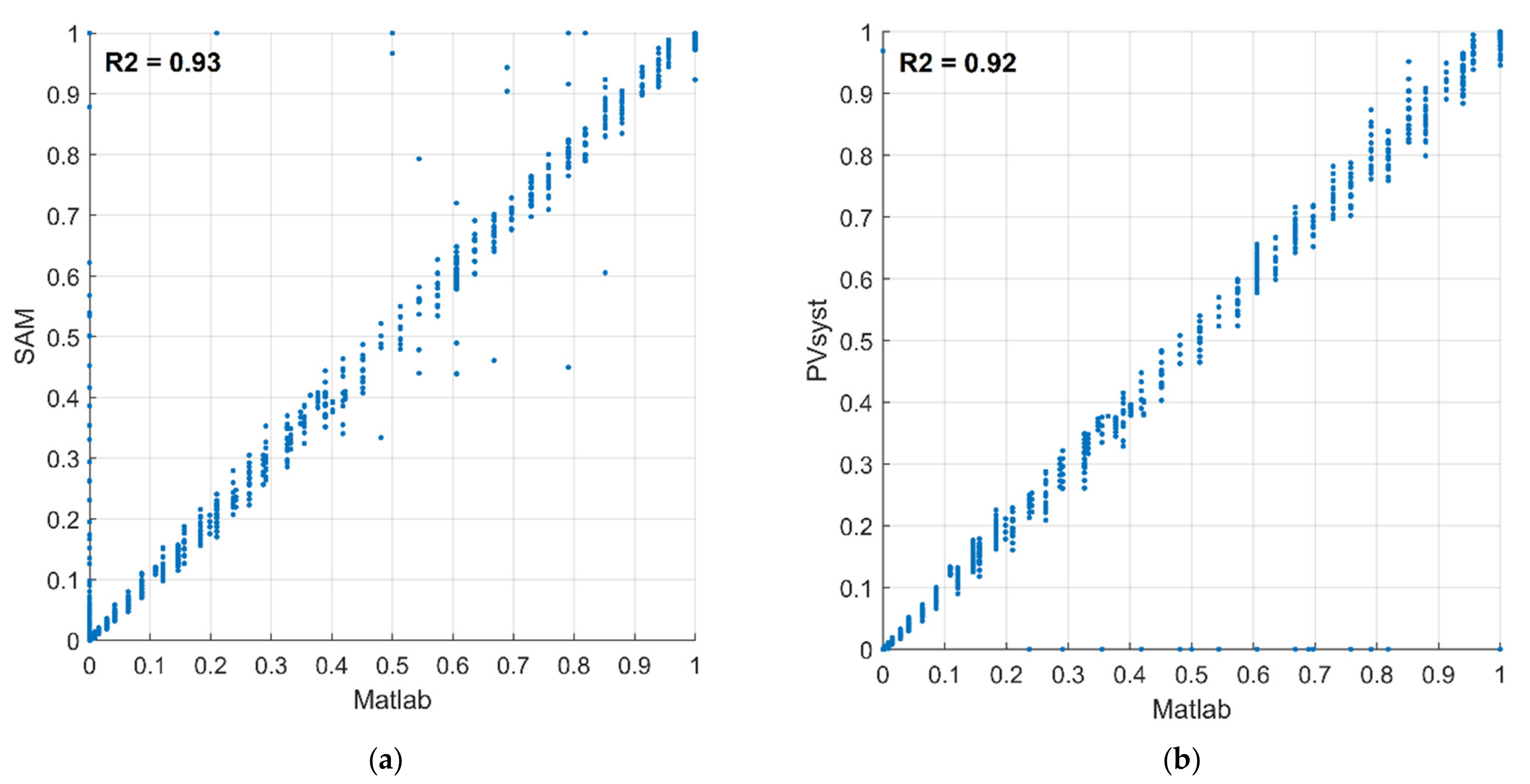
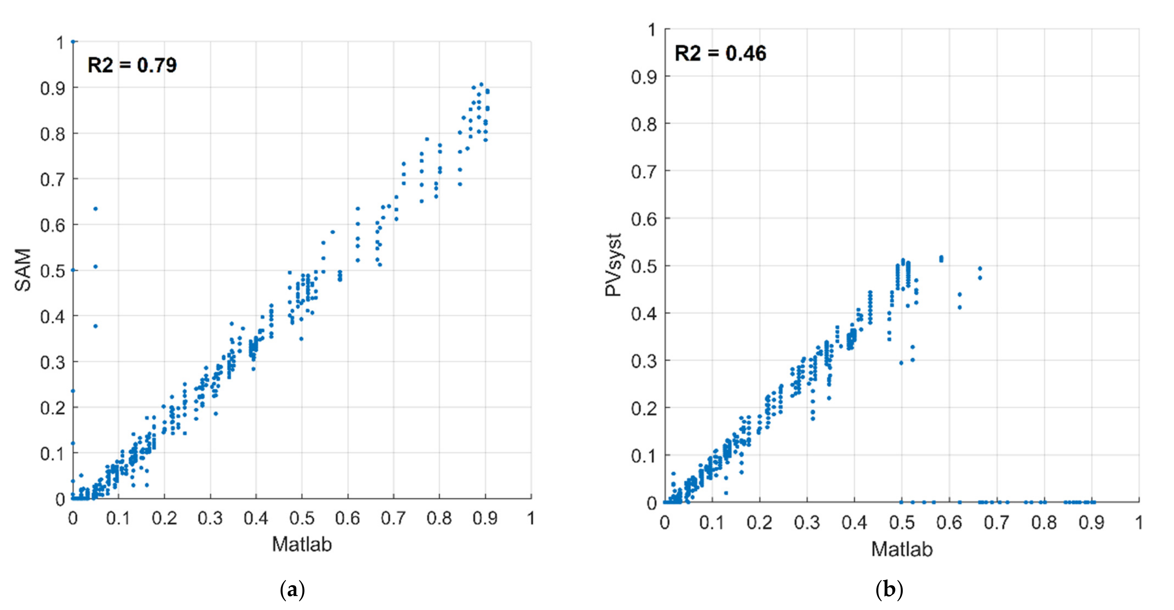
3. Validation
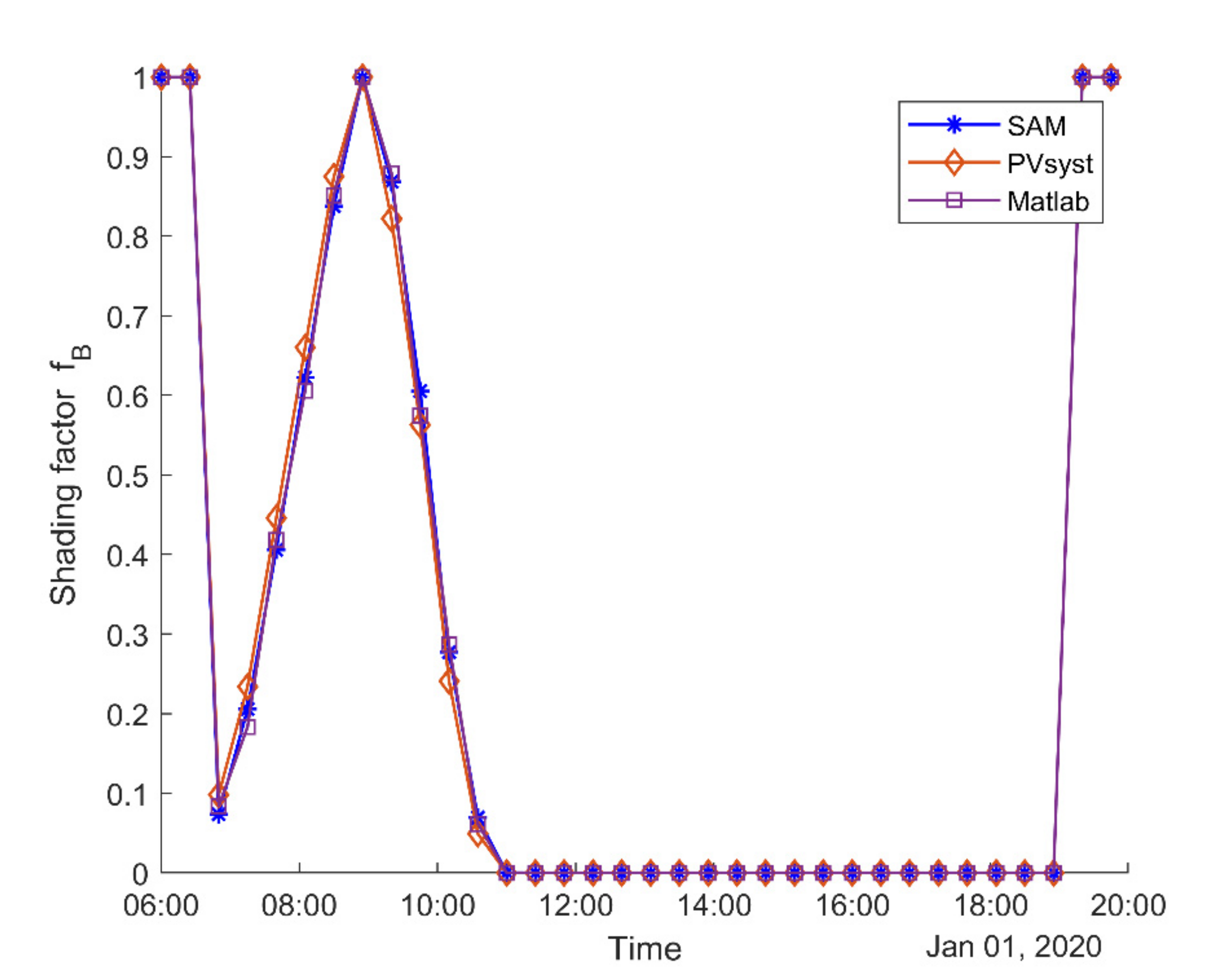
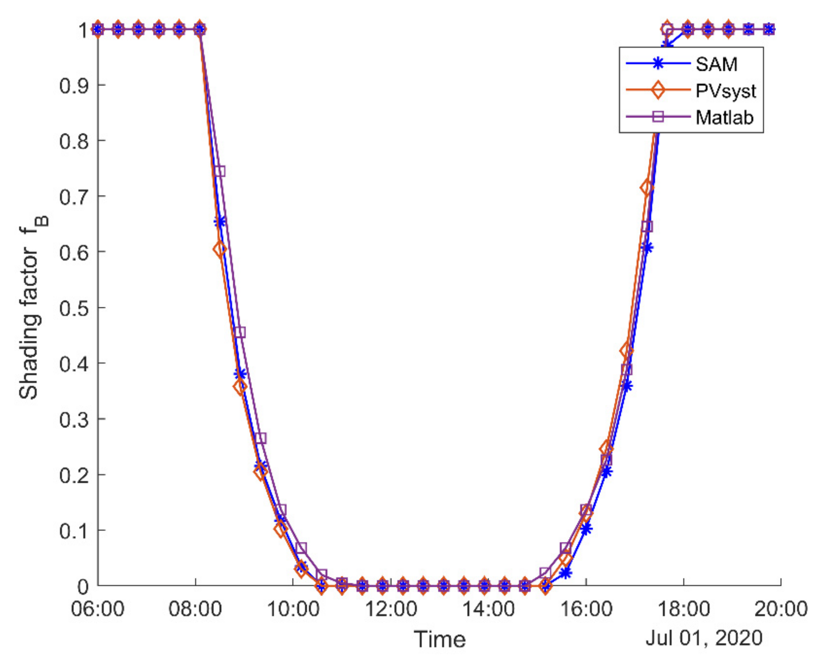
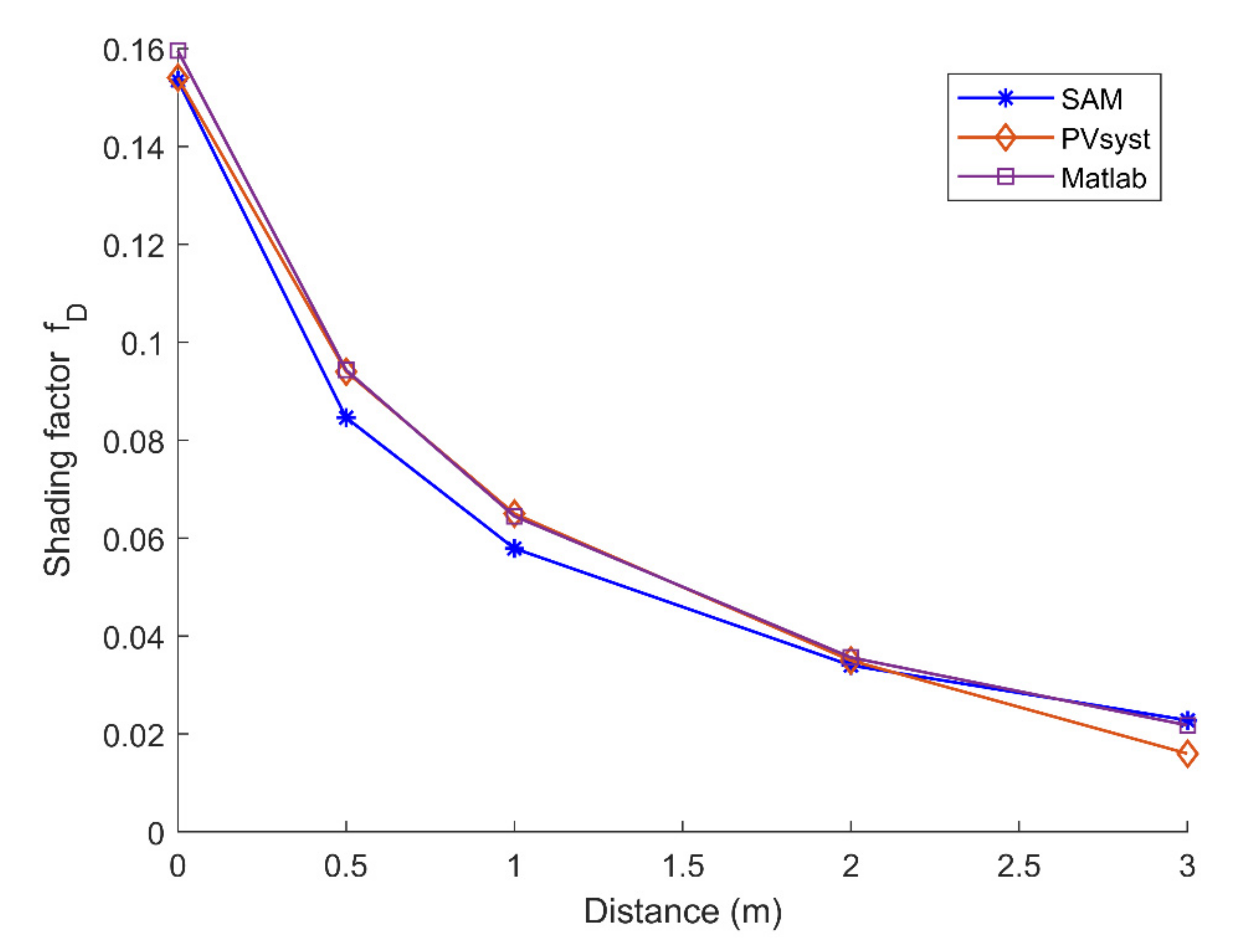
3.1. Direct Irradiance Shading Factor
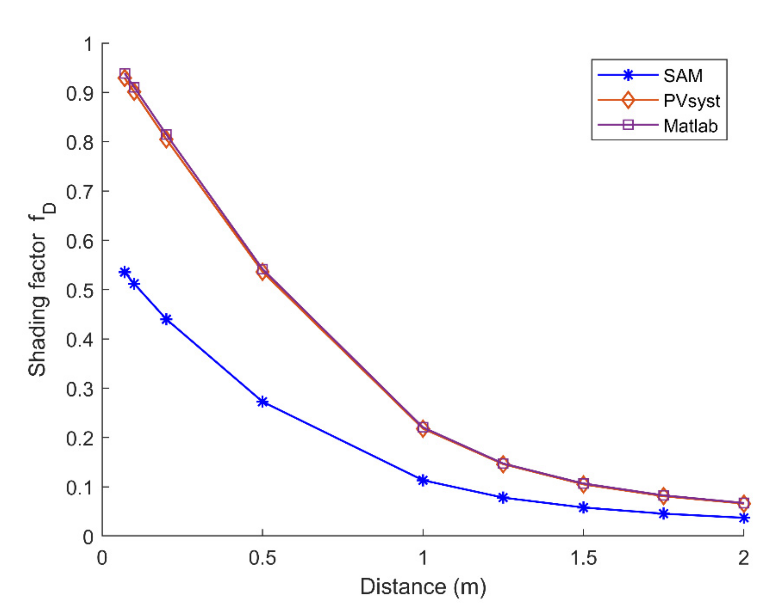
3.2. Diffuse Irradiance Shading Factor
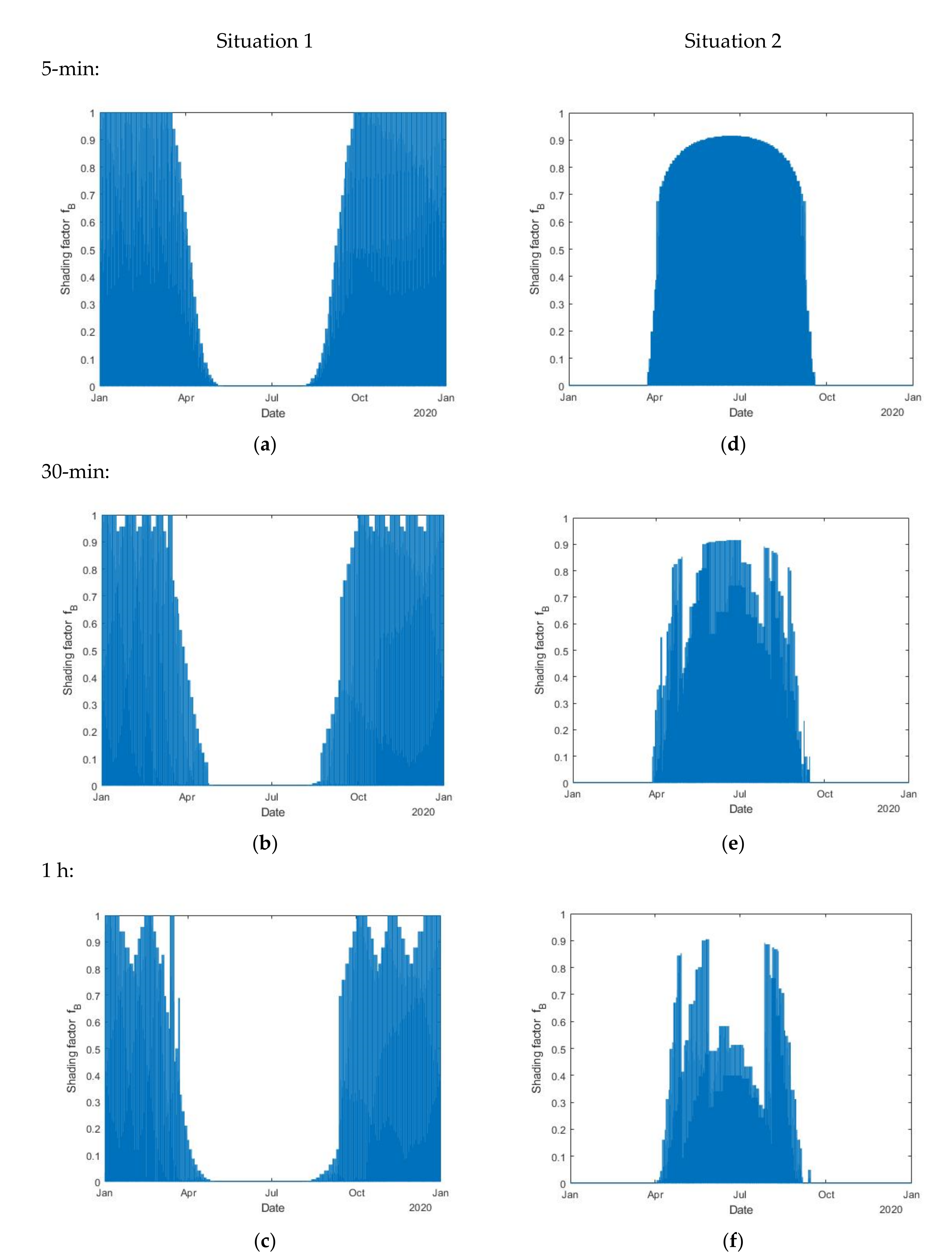
4. Results
5. Conclusions
Author Contributions
Funding
Institutional Review Board Statement
Informed Consent Statement
Data Availability Statement
Acknowledgments
Conflicts of Interest
Nomenclature
| Shading factor for direct irradiance | |
| Shading factor for diffuse irradiance | |
| Direct normal Irradiance | |
| Diffuse horizontal Irradiance | |
| Shaded area of the solar module | |
| Area of the module | |
| Vertices of each corner of the module | |
| Tilt angle of the module | |
| Azimuth angle of the module | |
| Rotation matrix about the y axis | |
| Rotation matrix about the z axis | |
| Obstacle vertex | |
| Projection of the obstacle vertex on the plane of the module | |
| Vector normal to the module plane | |
| Unit vector with the sun position in Cartesian coordinates | |
| Irradiance traversing the shaded area AS (diffuse) | |
| Irradiance reaching the area of the hemisphere AH (diffuse) | |
| Radiance of a sky element | |
| Angle of incidence | |
| Elevation angle of the sun |
References
- Green, M.A. Commercial progress and challenges for photovoltaics. Nat. Energy 2016, 1, 15015. [Google Scholar] [CrossRef]
- Eigensonne Das 1000 Dächer Programm. Available online: https://www.eigensonne.de/1000-daecher-programm/ (accessed on 22 October 2020).
- Strahs, G.; Tombari, C. Laying the Foundation for a Solar America: The Million Solar Roofs Initiative; National Renewable Energy Lab. (NREL): Golden, CO, USA, 2006. [Google Scholar] [CrossRef] [Green Version]
- North Carolina Federal Ministry of the Environment; N.S. (BMU) 100.000 Dächer-Solarstrom-Programm. Available online: https://www.bmu.de/pressemitteilung/100000-daecher-solarstrom-programm-kurz-vor-dem-ziel/ (accessed on 1 November 2020).
- Enkhardt, S. Österreichs 1-Million-Dächer-Programm für Photovoltaik nimmt Formen an. Available online: https://www.pv-magazine.de/2020/09/10/oesterreichs-1-million-daecher-programm-fuer-photovoltaik-nimmt-formen-an/ (accessed on 22 October 2020).
- Fraunhofer Institute for Solar Energy Systems (ISE). Photovoltaics Report. Available online: https://www.ise.fraunhofer.de/content/dam/ise/de/documents/publications/studies/Photovoltaics-Report.pdf (accessed on 16 September 2020).
- Ellabban, O.; Abu-Rub, H.; Blaabjerg, F. Renewable energy resources: Current status, future prospects and their enabling technology. Renew. Sustain. Energy Rev. 2014, 39, 748–764. [Google Scholar] [CrossRef]
- Decker, B.; Jahn, U. Performance of 170 grid connected PV plants in Northern Germany—Analysis of yields and optimization potentials. Sol. Energy 1997, 59, 127–133. [Google Scholar] [CrossRef]
- Quaschning, V.; Hanitsch, R. Irradiance calculation on shaded surfaces. Sol. Energy 1998, 62, 369–375. [Google Scholar] [CrossRef]
- MacAlpine, S.; Deline, C.; Dobos, A. Measured and estimated performance of a fleet of shaded photovoltaic systems with string and module-level inverters. Prog. Photovolt. Res. Appl. 2017, 25, 714–726. [Google Scholar] [CrossRef] [Green Version]
- Bayrak, F.; Ertürk, G.; Oztop, H.F. Effects of partial shading on energy and exergy efficiencies for photovoltaic panels. J. Clean. Prod. 2017, 164, 58–69. [Google Scholar] [CrossRef]
- Numan, A.H.; Dawood, Z.S.; Hussein, H.A. Theoretical and experimental analysis of photovoltaic module characteristics under different partial shading conditions. Int. J. Power Electron. Drive Syst. 2020, 11, 1508–1518. [Google Scholar] [CrossRef]
- Quaschning, V.; Hanitsch, R. Shade Calculations in Photovoltaic Systems. In Proceedings of the ISES Solar World Conference, Harare, Zimbabwe, 11–15 September 1995; pp. 1–5. [Google Scholar]
- Haberlin, H. Photovoltaics: System Design and Practice; John Wiley & Sons, Ltd.: Chichester, UK, 2012; ISBN 9781626239777. [Google Scholar]
- Teo, J.C.; Tan, R.H.G.; Mok, V.H.; Ramachandaramurthy, V.K.; Tan, C. Impact of Partial Shading on the P-V Characteristics and the Maximum Power of a Photovoltaic String. Energies 2018, 11, 1860. [Google Scholar] [CrossRef] [Green Version]
- MacAlpine, S.; Deline, C. Simplified method for modeling the impact of arbitrary partial shading conditions on PV array performance. In Proceedings of the IEEE 42nd Photovoltaic Specialist Conference (PVSC), New Orleans, LA, USA, 14–19 June 2015; pp. 1–6. [Google Scholar] [CrossRef]
- Cascone, Y.; Corrado, V.; Serra, V. Calculation procedure of the shading factor under complex boundary conditions. Sol. Energy 2011, 85, 2524–2539. [Google Scholar] [CrossRef]
- Melo, E.G.; Almeida, M.P.; Zilles, R.; Grimoni, J.A. Using a shading matrix to estimate the shading factor and the irradiation in a three-dimensional model of a receiving surface in an urban environment. Sol. Energy 2013, 92, 15–25. [Google Scholar] [CrossRef]
- Westbrook, O.; Reusser, M.; Collins, F. Diffuse shading losses in tracking photovoltaic systems. In Proceedings of the IEEE 40th Photovoltaic Specialist Conference (PVSC), Denver, CO, USA, 8–13 June 2014; pp. 0891–0896. [Google Scholar] [CrossRef]
- Li, Y.; Ding, D.; Liu, C.; Wang, C. A pixel-based approach to estimation of solar energy potential on building roofs. Energy Build. 2016, 129, 563–573. [Google Scholar] [CrossRef]
- National Reneable Energy Laboratory (NREL). System Advisor Model (SAM). Available online: https://sam.nrel.gov/ (accessed on 1 January 2021).
- PVsyst, S.A. PVsyst. Available online: https://www.pvsyst.com/ (accessed on 20 March 2021).
- Valentin Software PV*SOL. Available online: https://valentin-software.com/en/products/pvsol/ (accessed on 1 March 2021).
- Folsom Labs Helioscope. Available online: https://www.helioscope.com/ (accessed on 1 January 2021).
- Sandia National Laboratories. PV_LIB Toolbox. Available online: https://pvpmc.sandia.gov/applications/pv_lib-toolbox/ (accessed on 20 May 2020).
- Trejos Grisales, L.A.; Ramos Paja, C.A.; Saavedra Montes, A.J. Techniques for modeling photovoltaic systems under partial shading. Tecnura 2016, 20, 171–183. [Google Scholar] [CrossRef]
- PVsyst Shading Factor Table. Available online: https://www.pvsyst.com/help/shadings_factor_table.htm (accessed on 17 September 2020).
- Evans, P.R. Rotations and rotation matrices. Acta Crystallogr. Sect. D Biol. Crystallogr. 2001, 57, 1355–1359. [Google Scholar] [CrossRef] [PubMed] [Green Version]
- University of Texas. Equations of Planes. Available online: https://web.ma.utexas.edu/users/m408m/Display12-5-3.shtml (accessed on 4 July 2021).
- The MathWorks. Convhull. Available online: https://www.mathworks.com/help/matlab/ref/convhull.html (accessed on 21 October 2020).
- The MathWorks. Polyshape. Available online: https://www.mathworks.com/help/matlab/ref/polyshape.html?s_tid=doc_ta (accessed on 9 February 2020).
- The MathWorks. Intersect. Available online: https://www.mathworks.com/help/matlab/ref/double.intersect.html?s_tid=doc_ta (accessed on 15 February 2021).
- Sandia National Laboratories. Angle of Incidence. Available online: https://pvpmc.sandia.gov/modeling-steps/1-weather-design-inputs/plane-of-array-poa-irradiance/calculating-poa-irradiance/angle-of-incidence/ (accessed on 9 February 2020).
- Gilman, P. SAM Photovoltaic Model Technical Reference SAM Photovoltaic Model Technical Reference. Sol. Energy 2015, 63, 323–333. [Google Scholar] [CrossRef] [Green Version]


| Elevation\Azimuth | −150 | −100 | −50 | 0 | 50 | 100 | 150 |
|---|---|---|---|---|---|---|---|
| 0 | NaN | NaN | NaN | 1.00 | NaN | NaN | NaN |
| 10 | NaN | 0.00 | 0.86 | 0.92 | 0.86 | 0.00 | NaN |
| 20 | NaN | 0.20 | 0.74 | 0.82 | 0.74 | 0.20 | NaN |
| 30 | 0.00 | 0.30 | 0.66 | 0.74 | 0.66 | 0.30 | 0.00 |
| 40 | 0.00 | 0.34 | 0.61 | 0.68 | 0.61 | 0.34 | 0.00 |
| 50 | 0.01 | 0.37 | 0.56 | 0.62 | 0.56 | 0.37 | 0.01 |
| 60 | 0.19 | 0.39 | 0.52 | 0.57 | 0.52 | 0.39 | 0.19 |
| 70 | 0.29 | 0.40 | 0.49 | 0.52 | 0.49 | 0.40 | 0.29 |
| 80 | 0.37 | 0.41 | 0.46 | 0.48 | 0.46 | 0.41 | 0.37 |
| 90 | 0.42 | 0.42 | 0.42 | 0.42 | 0.42 | 0.42 | 0.42 |
| Parameters | Situation 1 (East Obstacle) | Situation 2 (Infinite Row) |
|---|---|---|
| Obstacle Geometry | ||
| Width (m) | 1 | 30 |
| Length (m) | 1 | 0.05 |
| Height (m) | 5 | 1 |
| Tilt angle (°) | 0 | 60 |
| Azimuth angle (°) | 0 | 0 |
| Distance of separation from module (m) | 2 | 2 |
| Module Geometry | ||
| Width (m) | 2 | |
| Height (m) | 1 | |
| Tilt angle (°) | 30 | |
| Azimuth angle (°) | 0 | |
| East Obstacle | ||||||||
|---|---|---|---|---|---|---|---|---|
| Month | SAM | PVsyst | ||||||
| MBE | MBEr (%) | RMSE | RMSEr (%) | MBE | MBEr (%) | RMSE | RMSEr (%) | |
| September | −0.001 | 14 | 0.0107 | 35 | 0.0006 | 17 | 0.0058 | 29 |
| October | −0.0004 | −17 | 0.0079 | 11 | 0.0000 | 0 | 0.0052 | 7 |
| November | −0.0002 | 11 | 0.0073 | 9 | −0.0001 | 4 | 0.006 | 7 |
| December | −0.0004 | −9 | 0.0195 | 22 | 0.0004 | 1 | 0.0062 | 7 |
| January | 0.0000 | −20 | 0.0073 | 8 | 0.0009 | 1 | 0.0113 | 13 |
| February | −0.0219 | −20 | 0.1318 | 134 | 0.0011 | 28 | 0.0084 | 14 |
| March | −0.0095 | −23 | 0.0721 | 149 | −0.001 | 12 | 0.0367 | 126 |
| April | −0.0016 | −52 | 0.0082 | 239 | 0.0001 | 74 | 0.0013 | 79 |
| Infinite Row | ||||||||
|---|---|---|---|---|---|---|---|---|
| Month | SAM | PVsyst | ||||||
| MBE | MBEr (%) | RMSE | RMSEr (%) | MBE | MBEr (%) | RMSE | RMSEr (%) | |
| April | 0.005 | 89 | 0.021 | 118 | 0.002 | 35 | 0.013 | 159 |
| May | 0.008 | 88 | 0.024 | 57 | 0.004 | 54 | 0.015 | 62 |
| June | 0.008 | 40 | 0.021 | 54 | 0.005 | 18 | 0.015 | 34 |
| July | 0.006 | 60 | 0.016 | 49 | 0.004 | 41 | 0.012 | 41 |
| August | 0.003 | 33 | 0.015 | 38 | 0.004 | 68 | 0.021 | 181 |
| September | −0.002 | −29 | 0.032 | 1005 | 0.000 | 216 | 0.006 | 1768 |
| East Obstacle | ||||
|---|---|---|---|---|
| Distance (m) | SAM | PVsyst | ||
| MBE | MBEr (%) | MBE | MBEr (%) | |
| 0 | 0.0061 | 3.94 | 0.0056 | 3.61 |
| 0.5 | 0.0097 | 11.50 | 0.0003 | 0.35 |
| 1 | 0.0066 | 11.36 | −0.0005 | −0.80 |
| 2 | 0.0016 | 4.79 | 0.0006 | 1.80 |
| 3 | −0.0010 | −4.45 | 0.0058 | 36.16 |
| Infinite Row | ||||
|---|---|---|---|---|
| Distance (m) | SAM | PVsyst | ||
| MBE | MBEr (%) | MBE | MBEr (%) | |
| 0.07 | 0.4034 | 75.35 | 0.0098 | 1.06 |
| 0.1 | 0.3986 | 77.88 | 0.0094 | 1.04 |
| 0.2 | 0.3748 | 85.17 | 0.0098 | 1.21 |
| 0.5 | 0.2691 | 98.70 | 0.0057 | 1.06 |
| 1 | 0.1073 | 94.73 | 0.0026 | 1.21 |
| 1.25 | 0.0692 | 88.56 | 0.0013 | 0.87 |
| 1.5 | 0.0487 | 84.03 | 0.0017 | 1.66 |
| 1.75 | 0.0372 | 81.71 | 0.0017 | 2.07 |
| 2 | 0.0300 | 80.72 | 0.0012 | 1.86 |
Publisher’s Note: MDPI stays neutral with regard to jurisdictional claims in published maps and institutional affiliations. |
© 2021 by the authors. Licensee MDPI, Basel, Switzerland. This article is an open access article distributed under the terms and conditions of the Creative Commons Attribution (CC BY) license (https://creativecommons.org/licenses/by/4.0/).
Share and Cite
Silva, M.; Roberts, J.J.; Prado, P.O. Calculation of the Shading Factors for Solar Modules with MATLAB. Energies 2021, 14, 4713. https://doi.org/10.3390/en14154713
Silva M, Roberts JJ, Prado PO. Calculation of the Shading Factors for Solar Modules with MATLAB. Energies. 2021; 14(15):4713. https://doi.org/10.3390/en14154713
Chicago/Turabian StyleSilva, Martín, Justo Jose Roberts, and Pedro Osvaldo Prado. 2021. "Calculation of the Shading Factors for Solar Modules with MATLAB" Energies 14, no. 15: 4713. https://doi.org/10.3390/en14154713