
On-Line Control of Stresses in the Power Unit Pressure Elements Taking Account of Variable Heat Transfer Conditions


Abstract
:1. Introduction
2. Algorithms for Stress Calculation in Turbine Elements
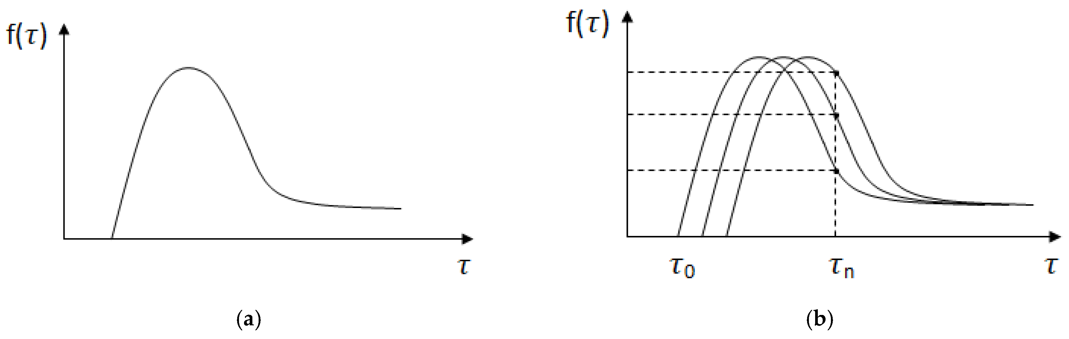
2.1. Agorithms Based on Green’s Functions
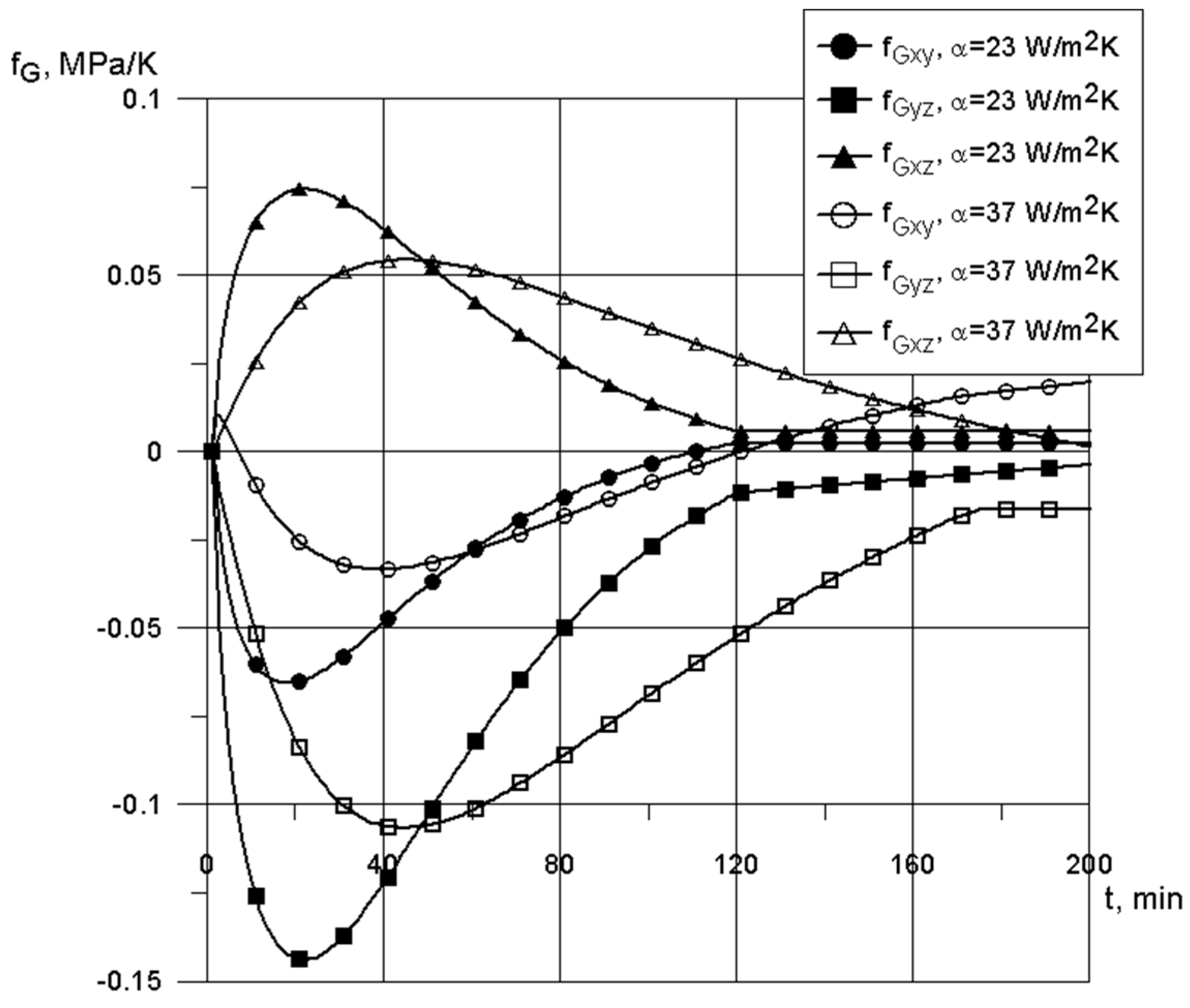
2.2. Modification of the Algorith for Thermal Stress Determination
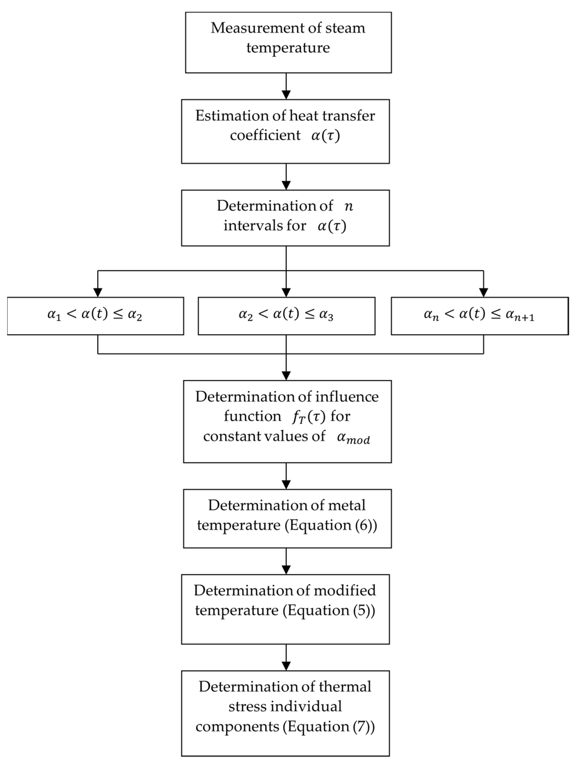
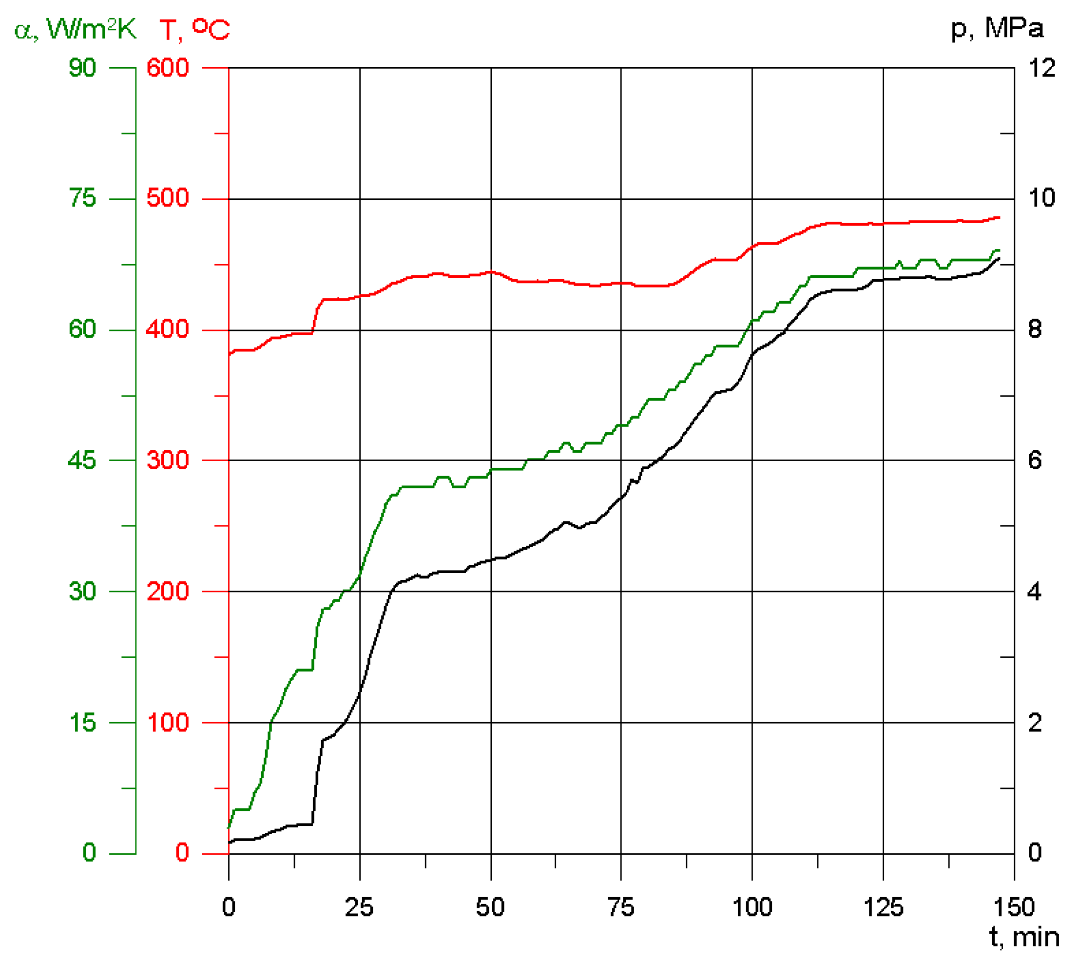
3. Determination of Heat Transfer Coefficients
4. Application of the Proposed Algorithm for Stress Calculation in Turbine Pressure Components
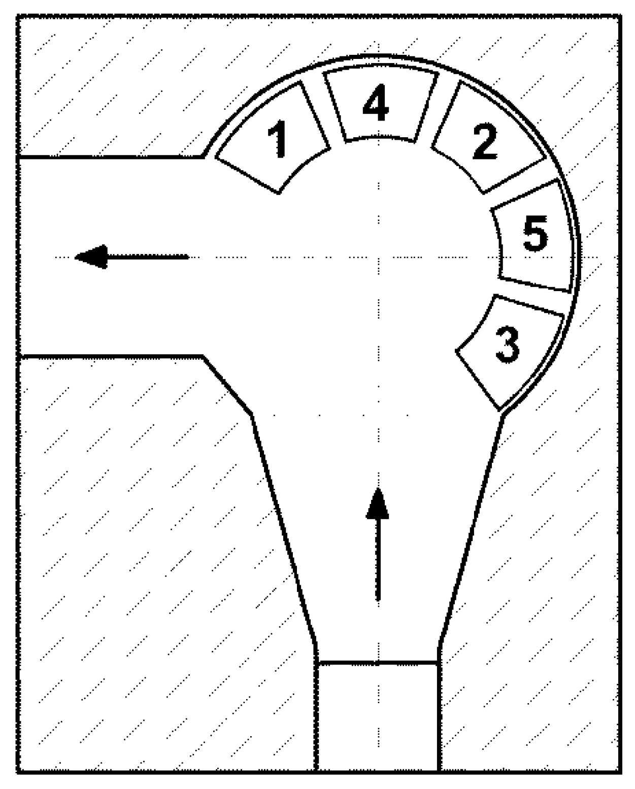
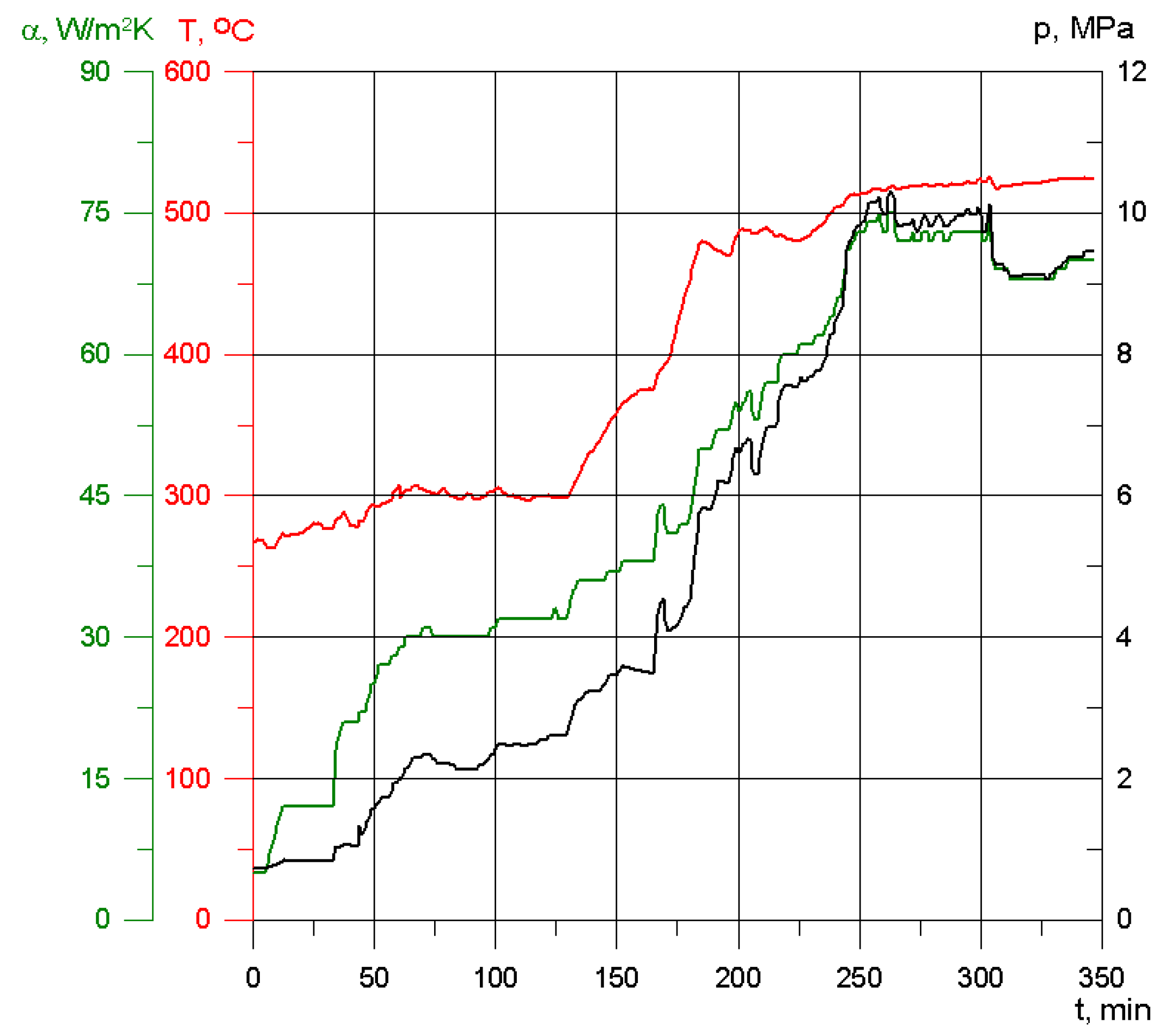
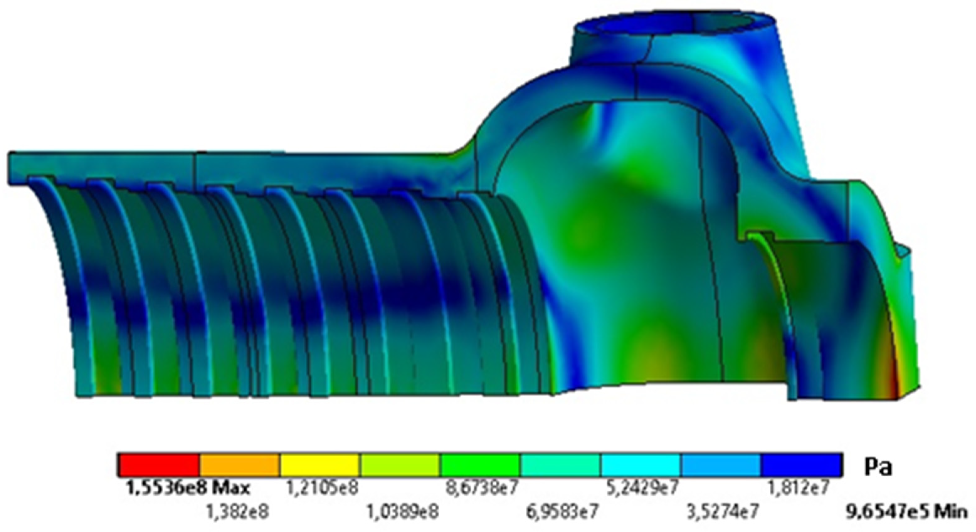
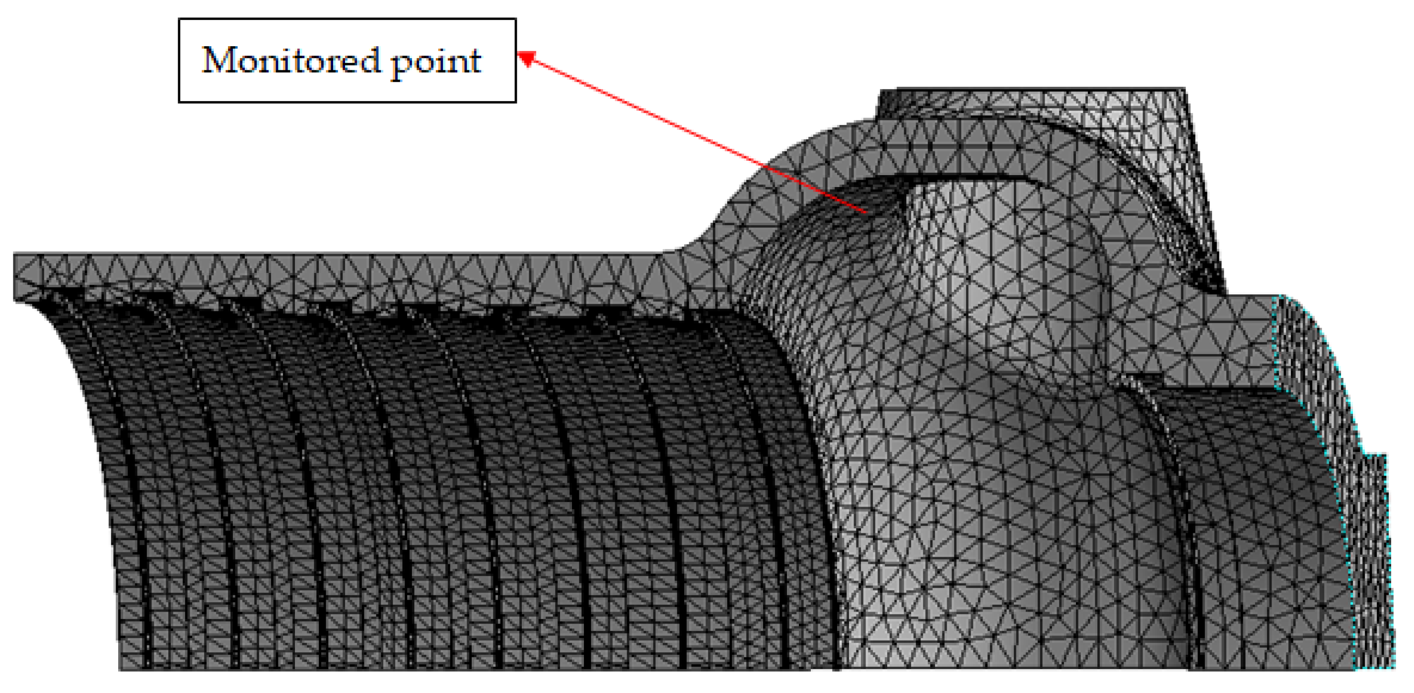
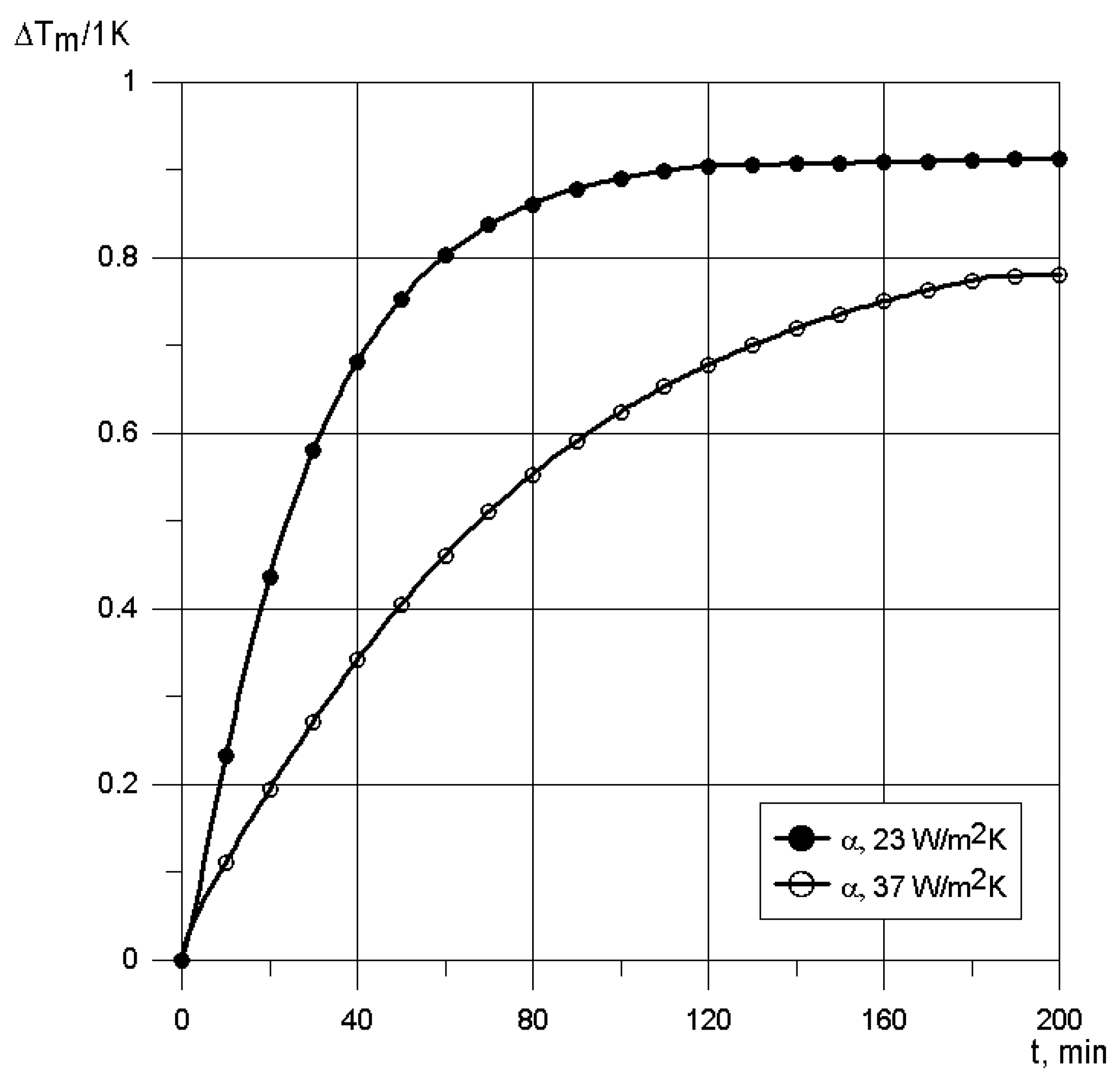
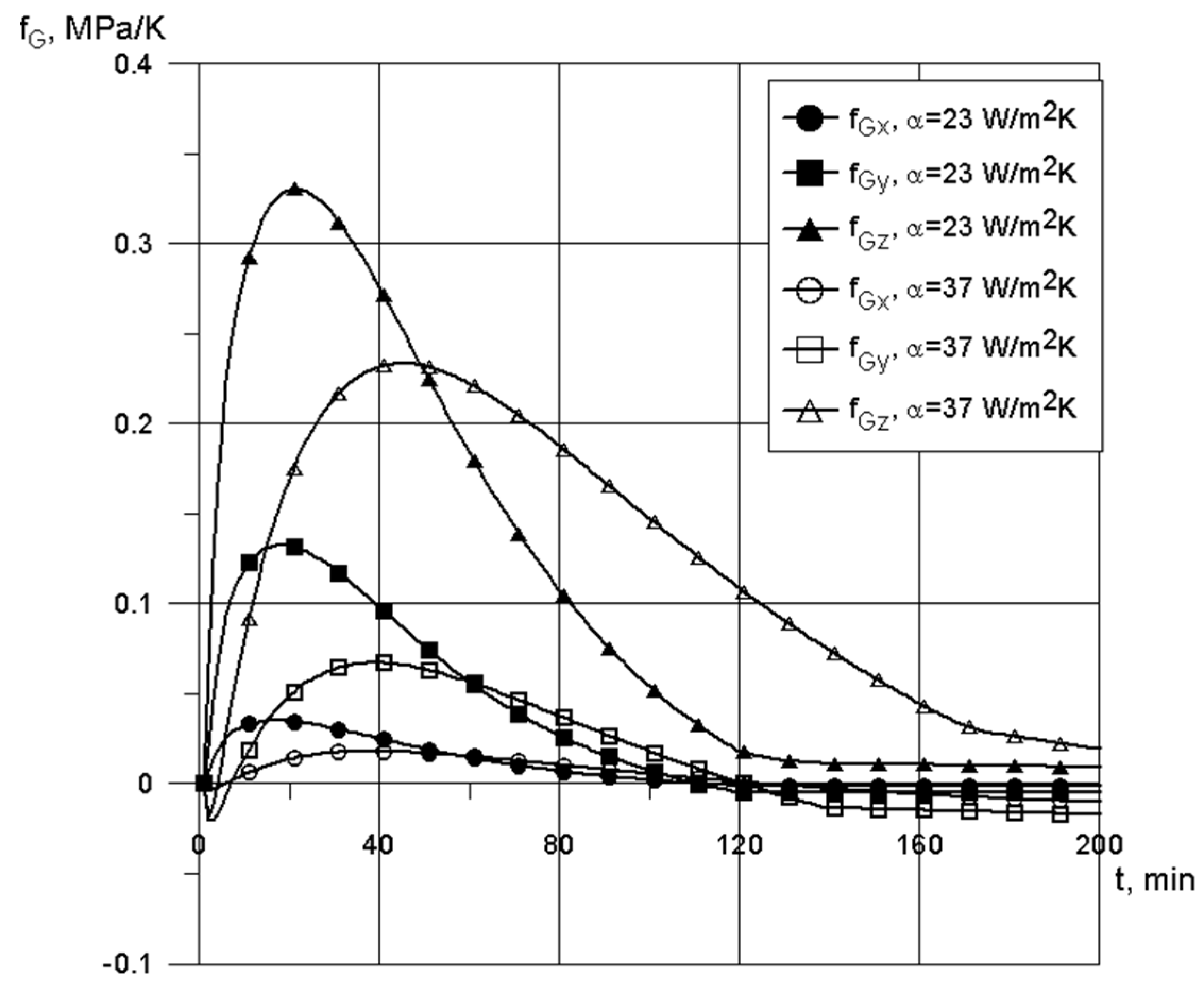
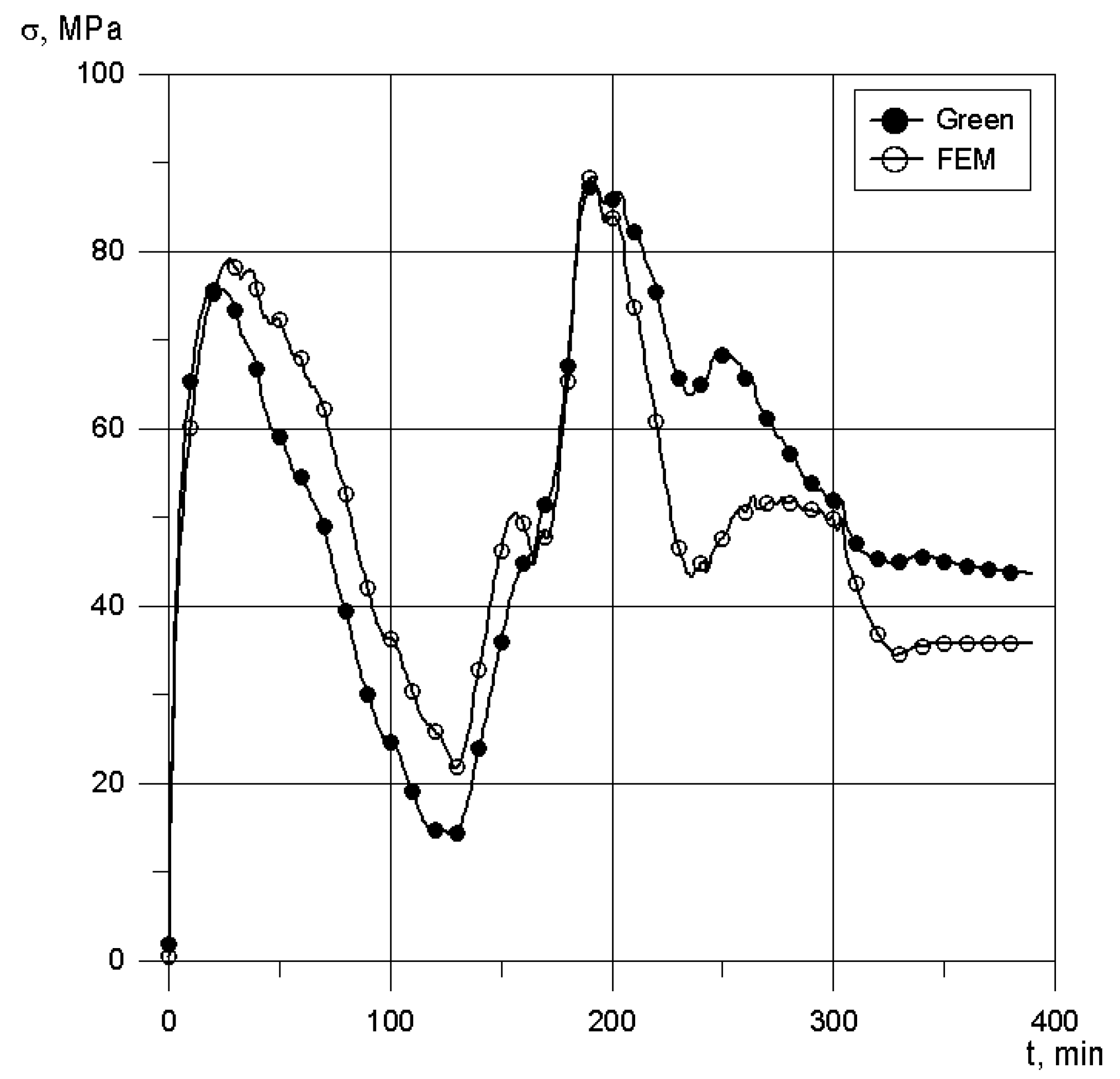
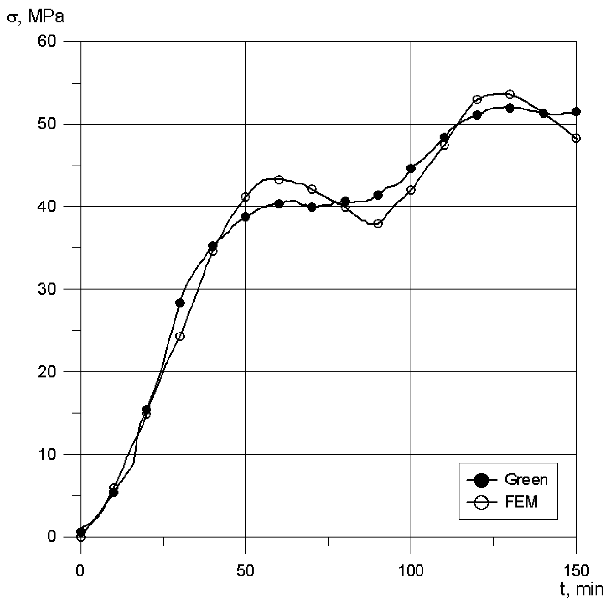
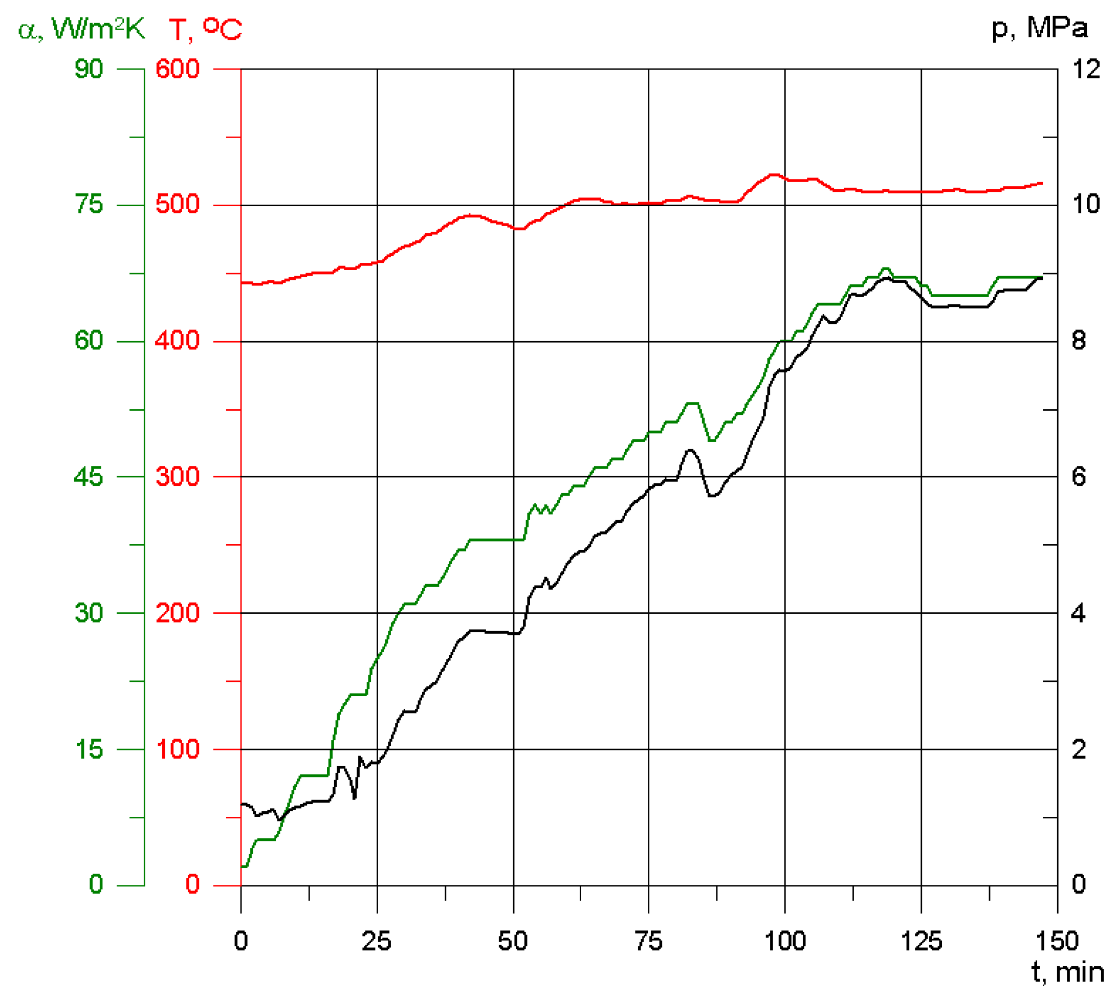
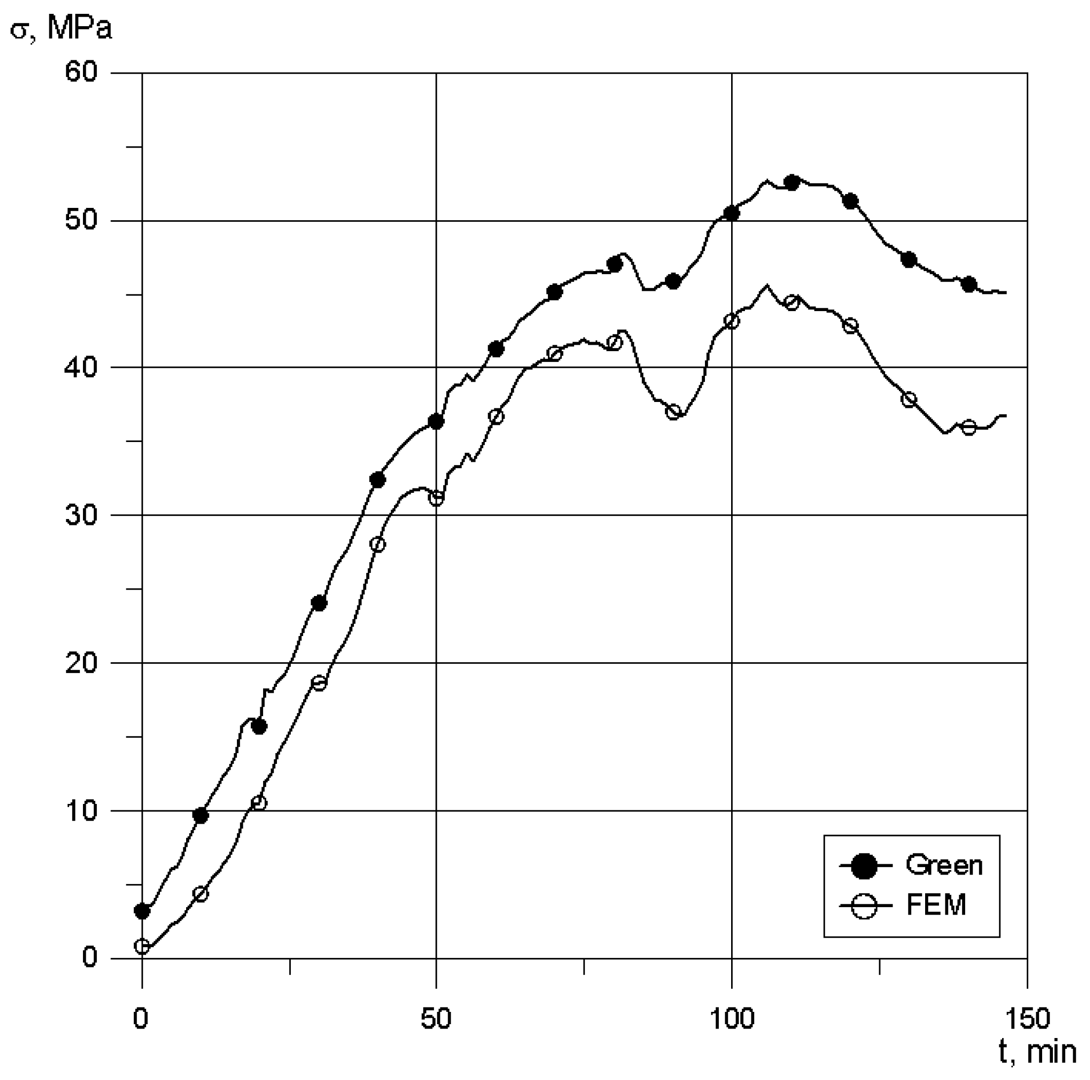
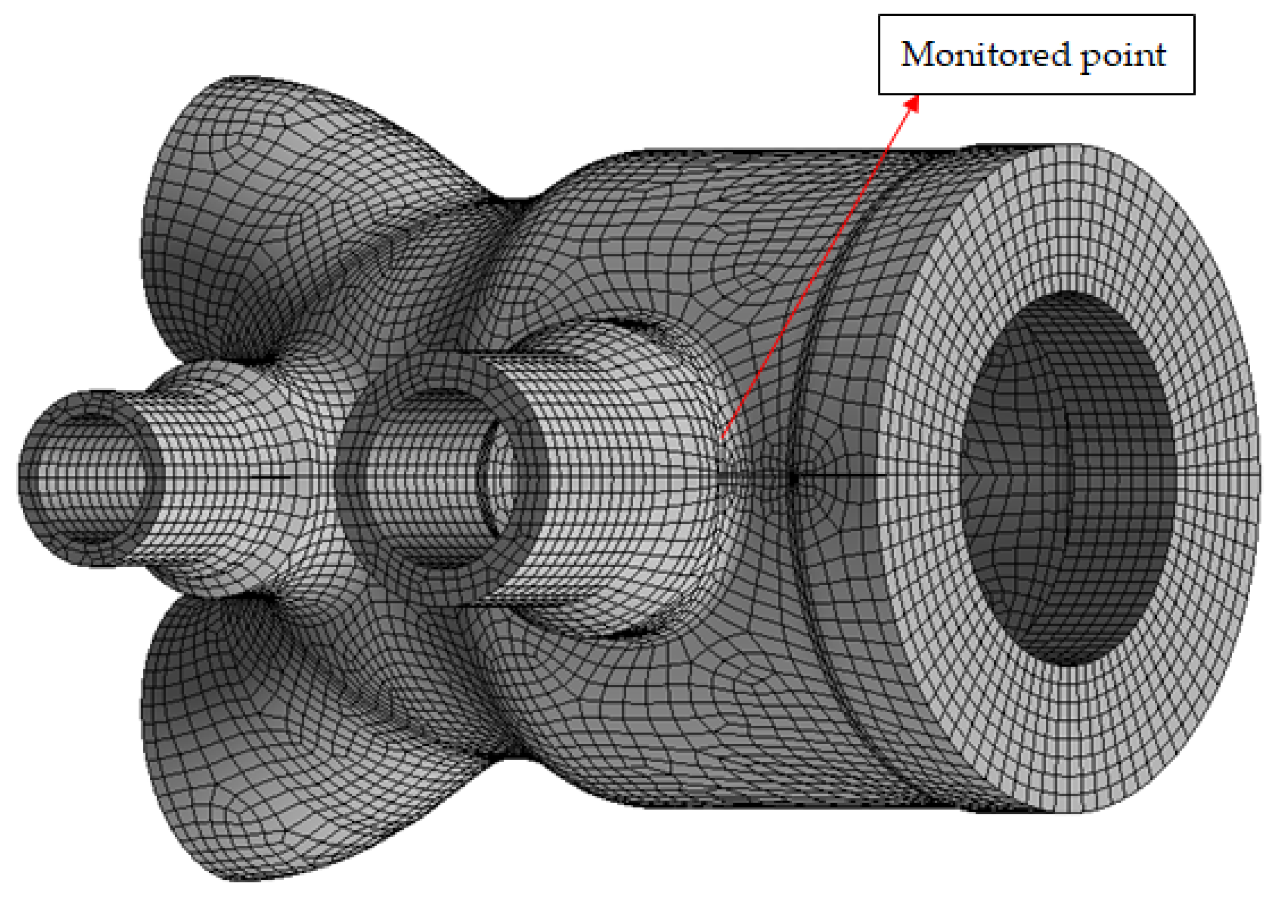
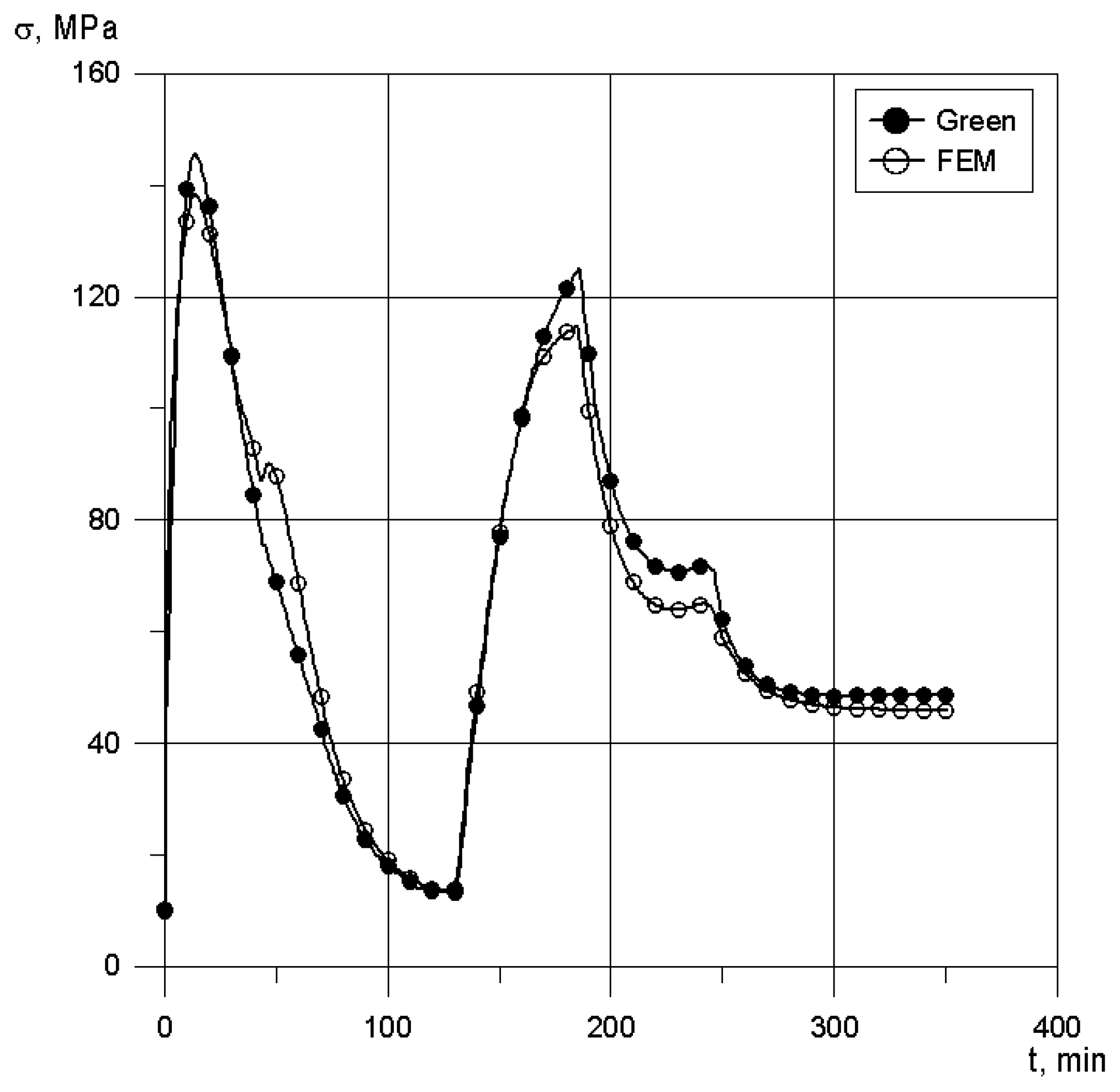
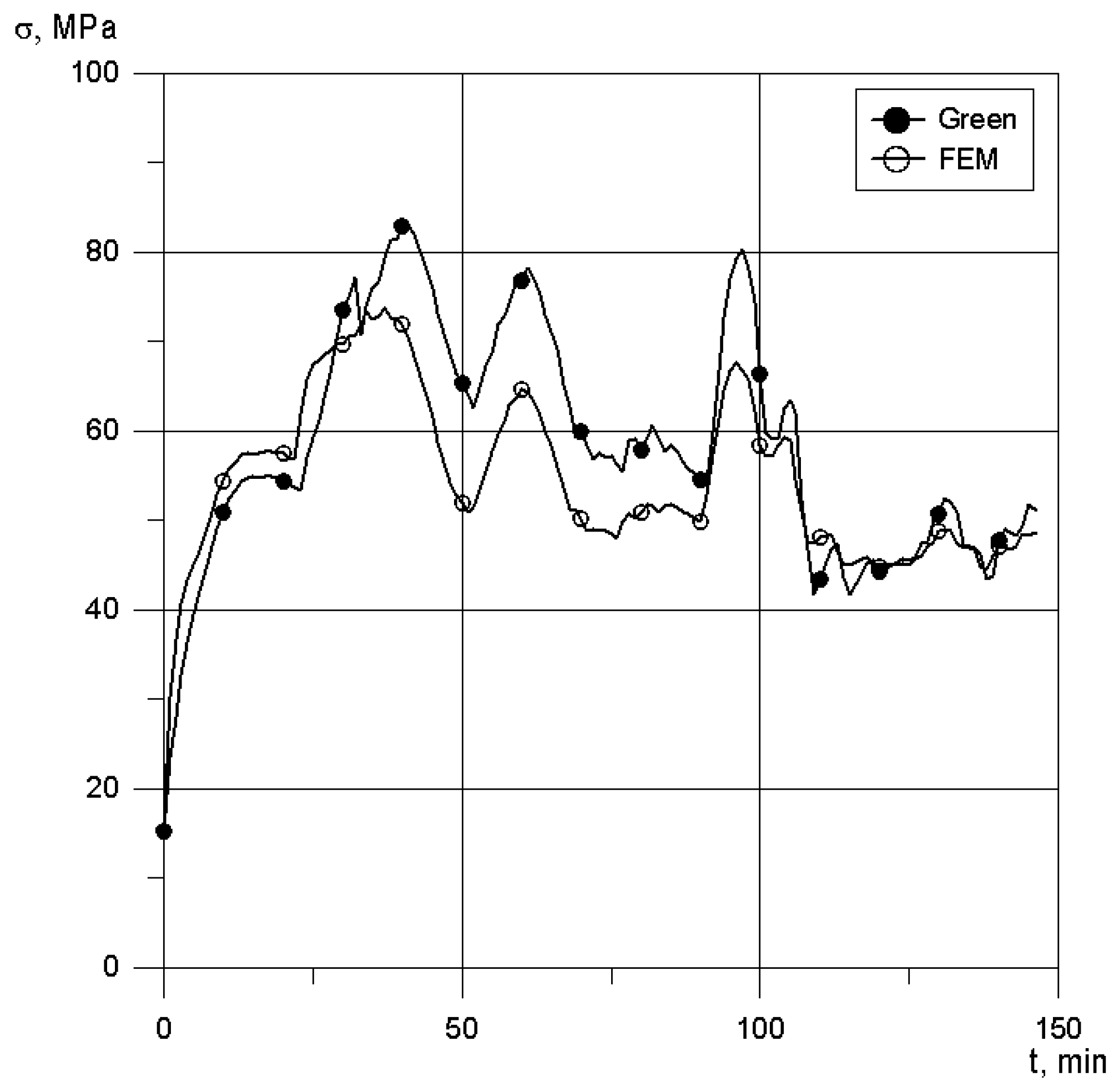
4.1. Turbine Inner Casing
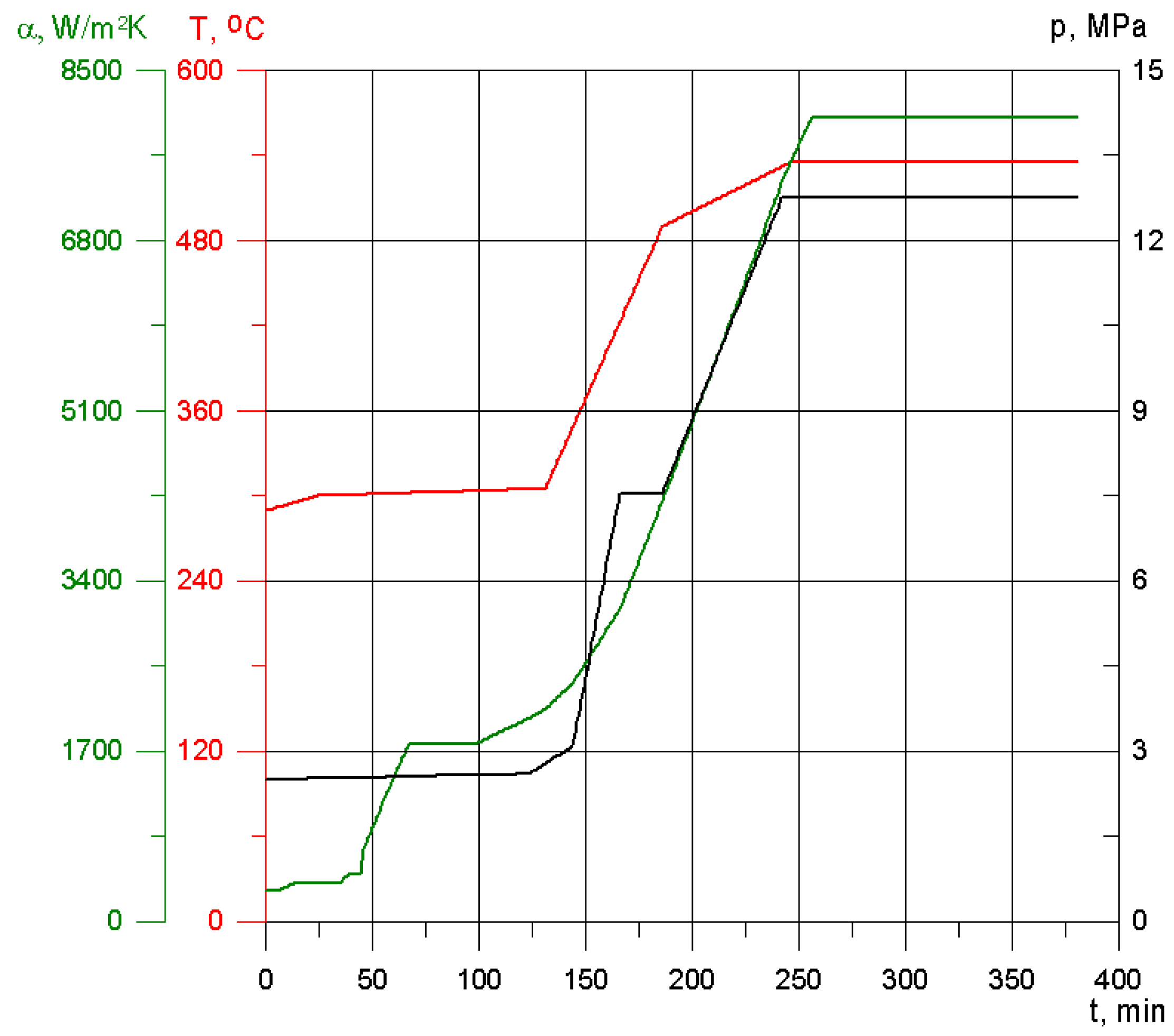
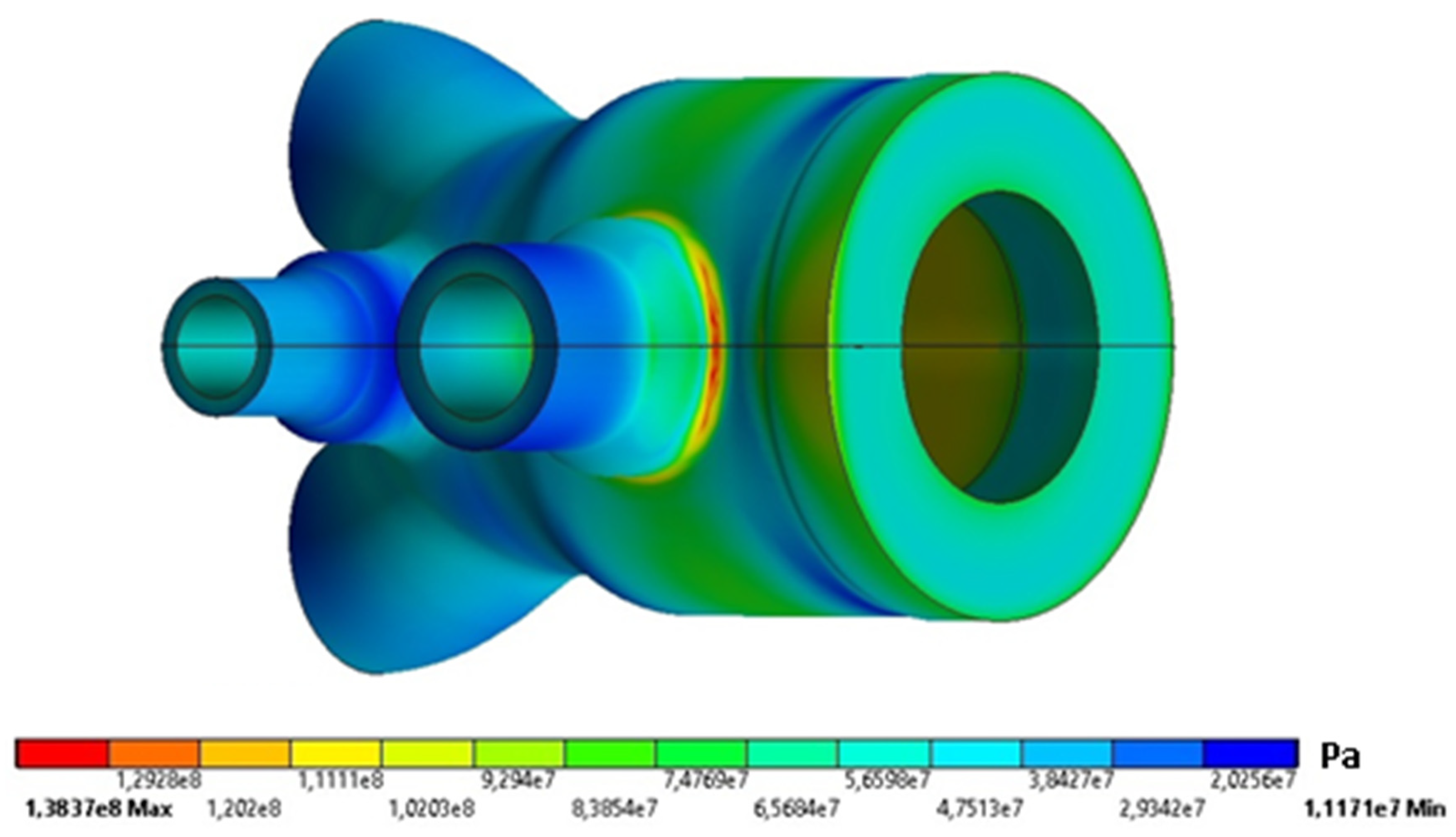
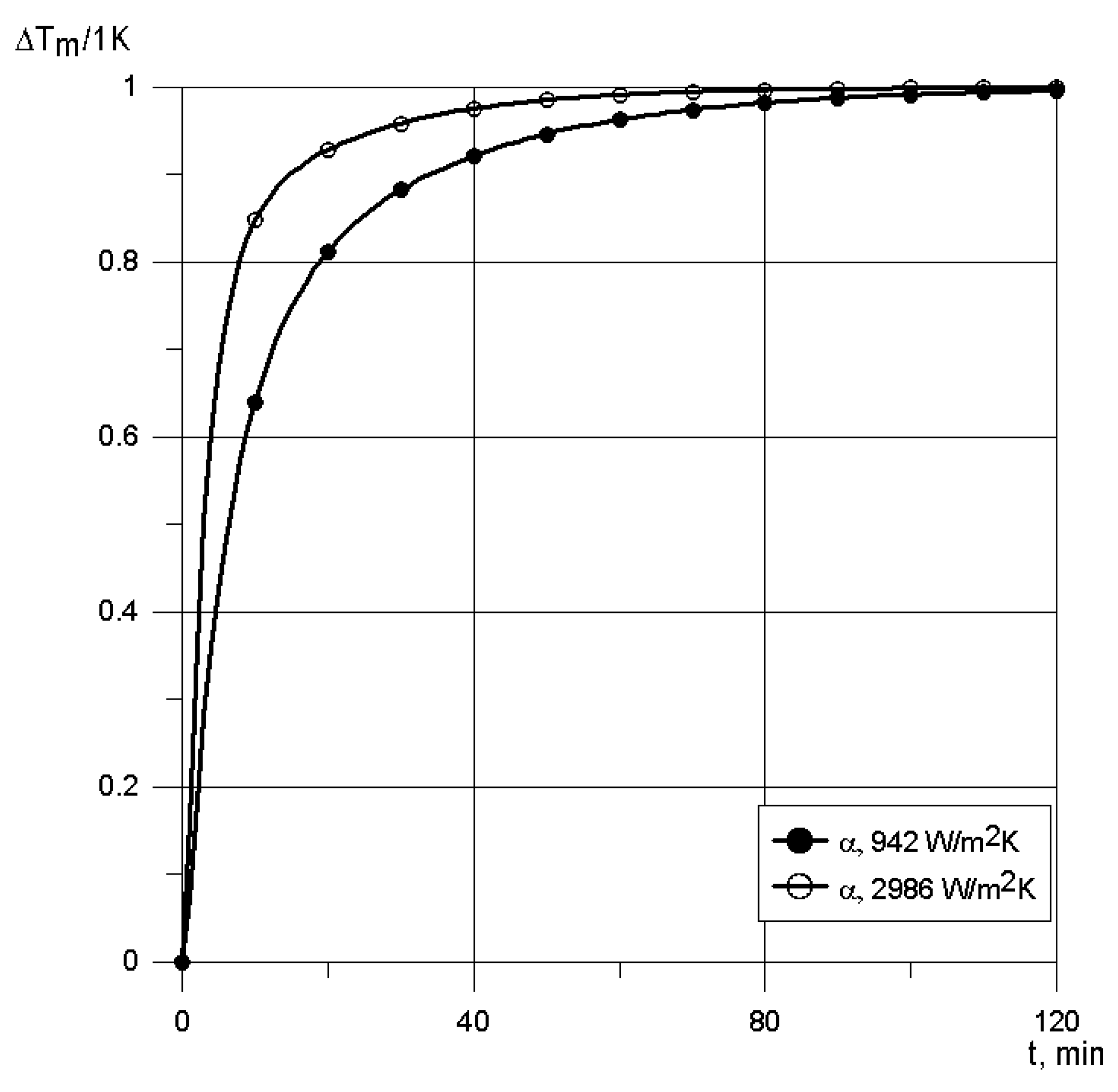
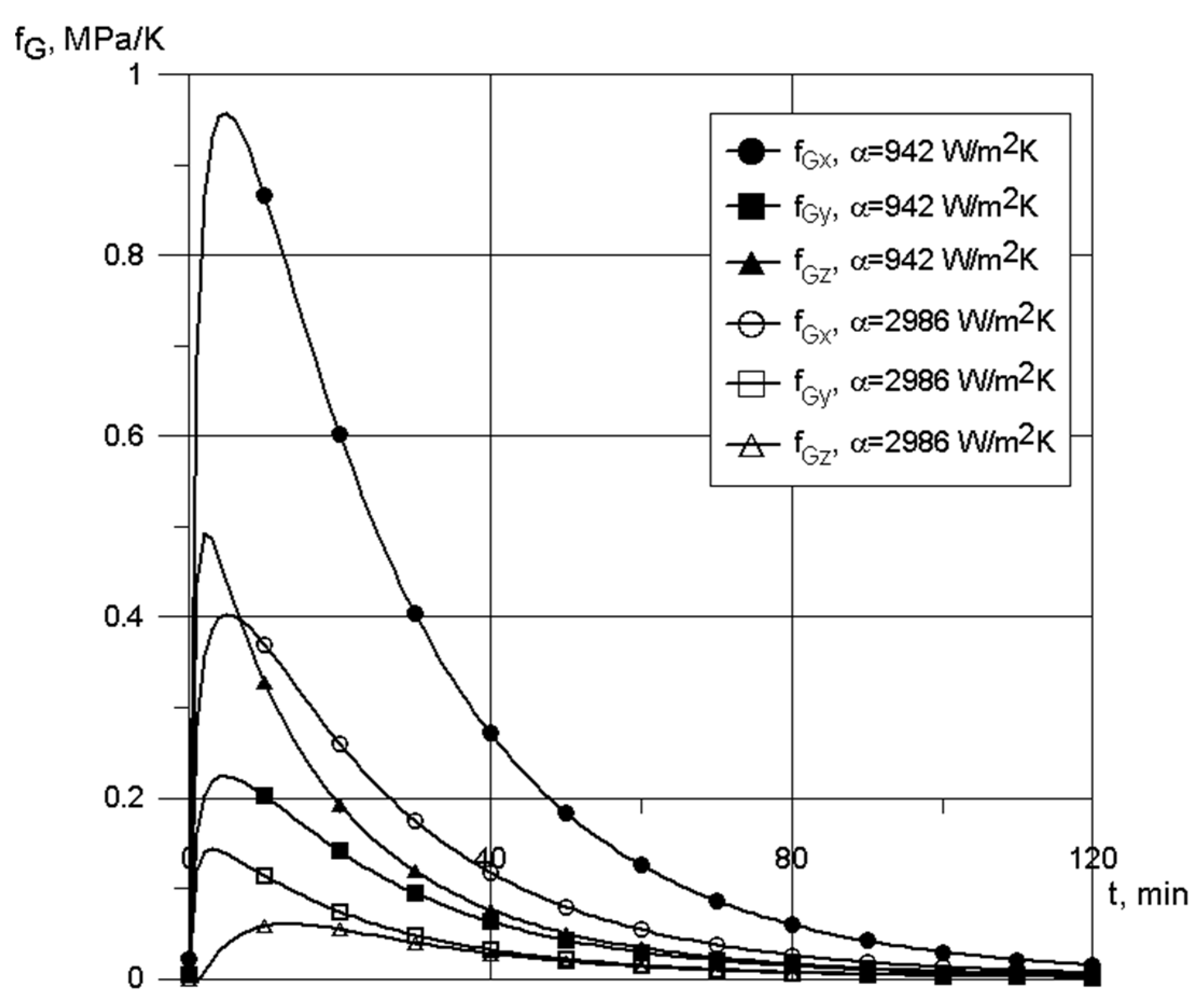
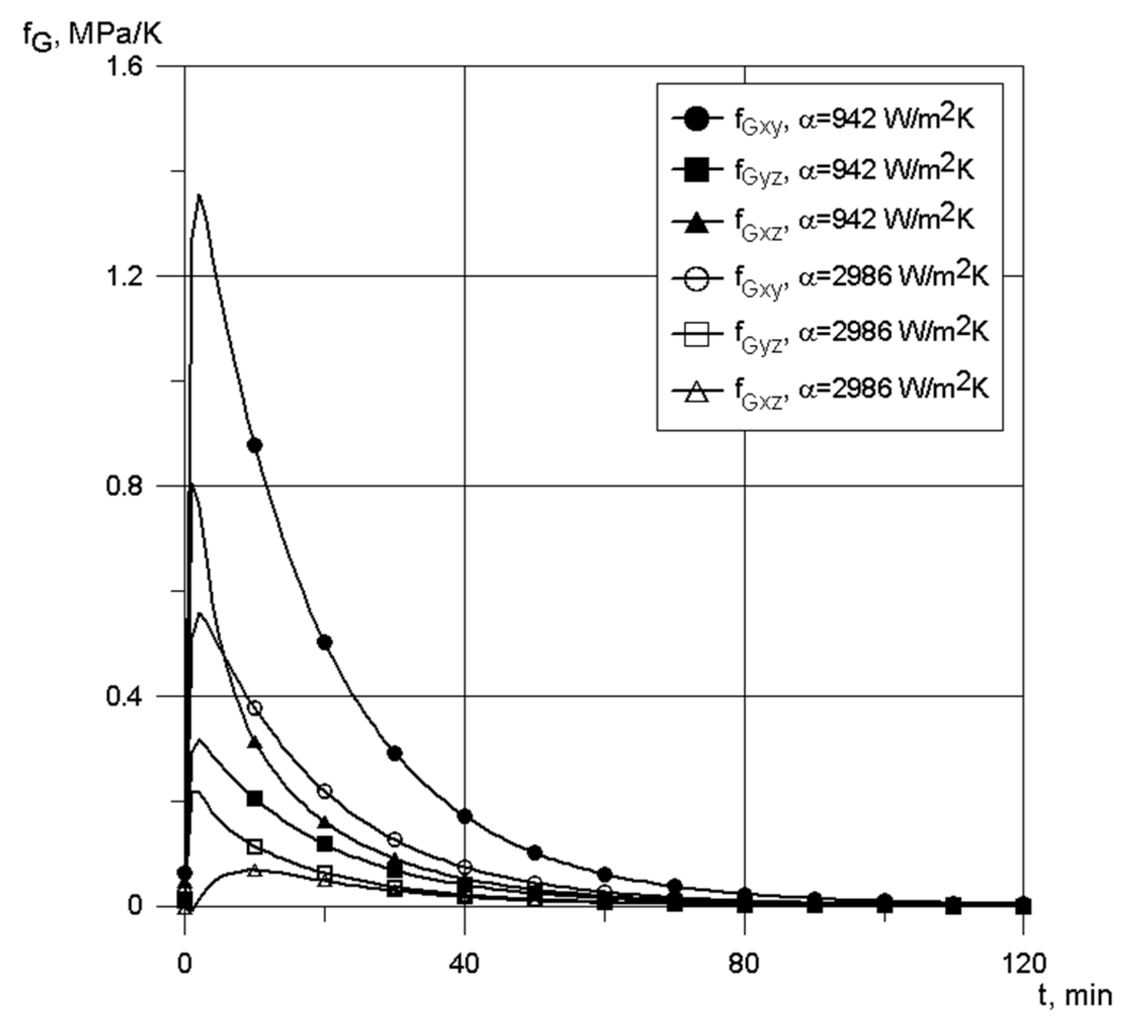
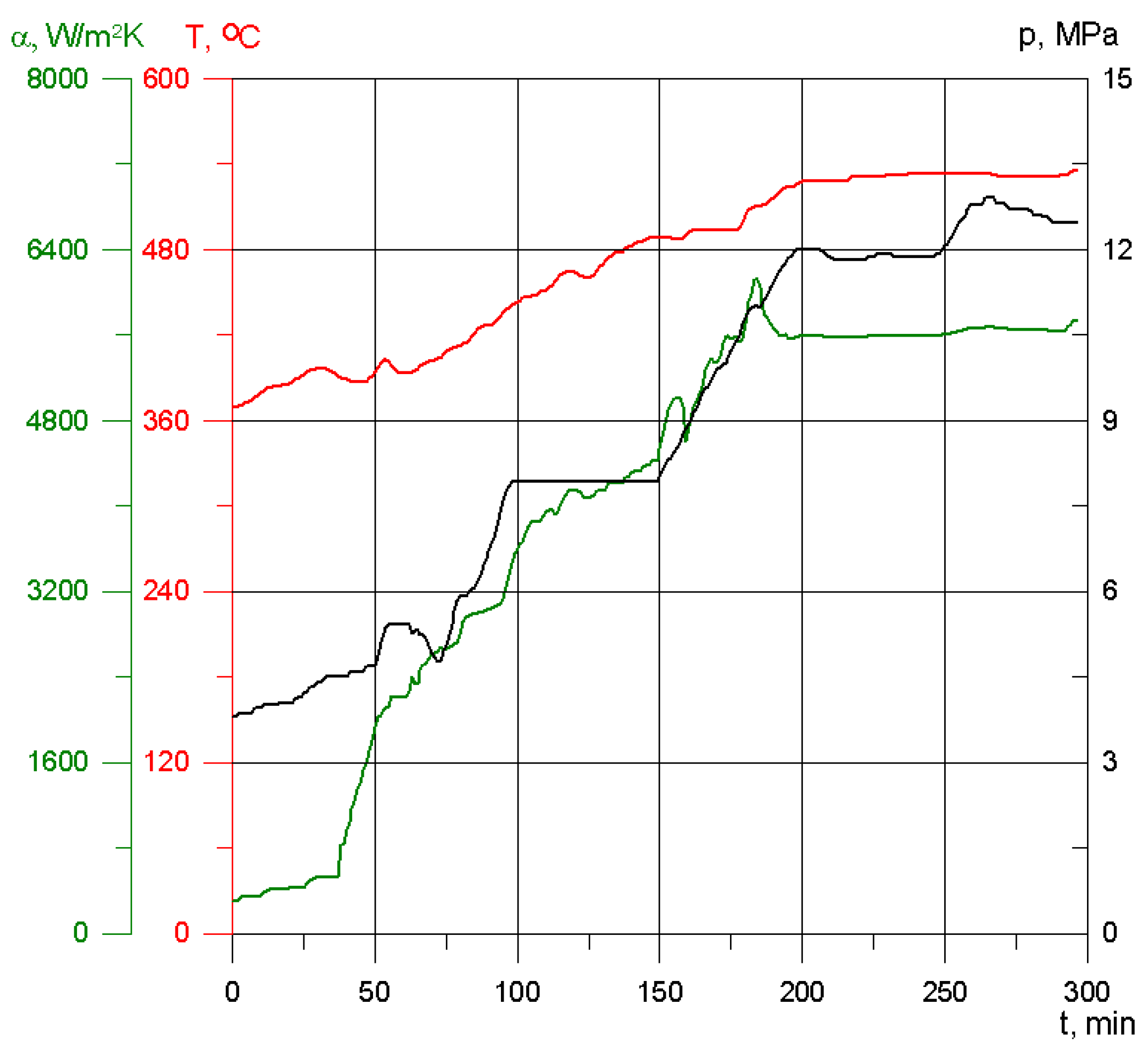
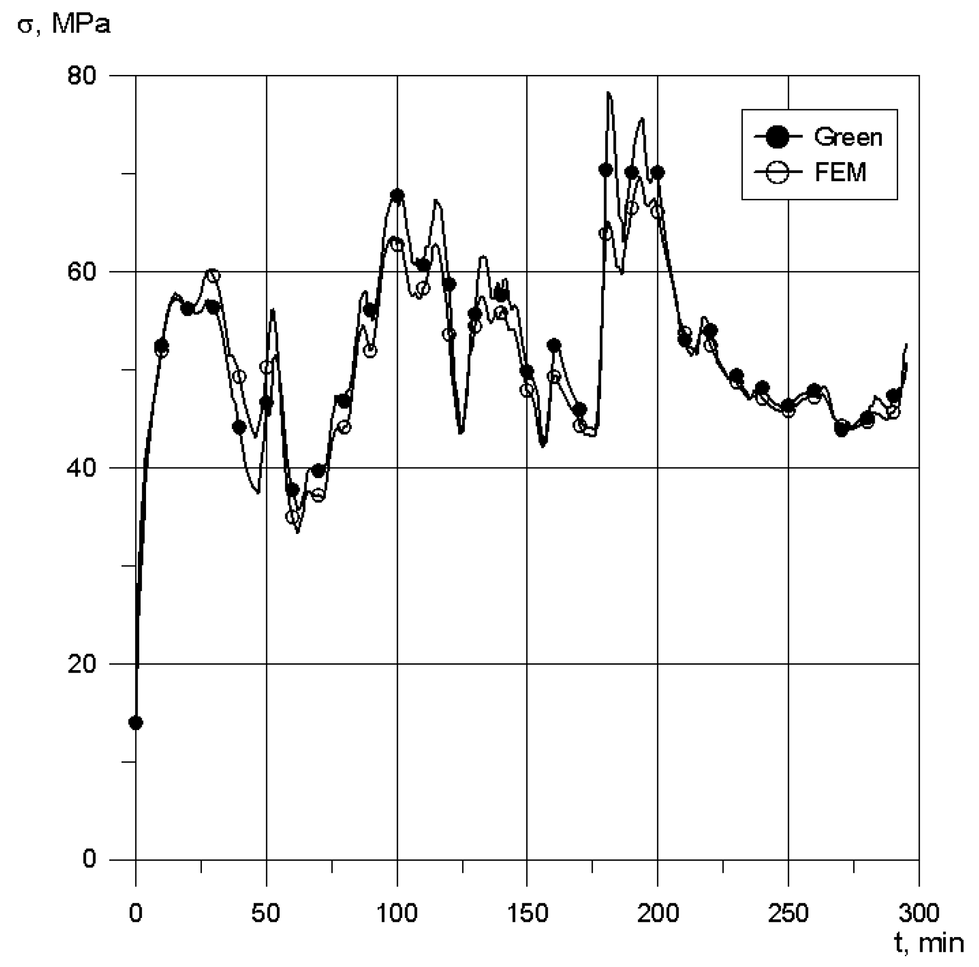
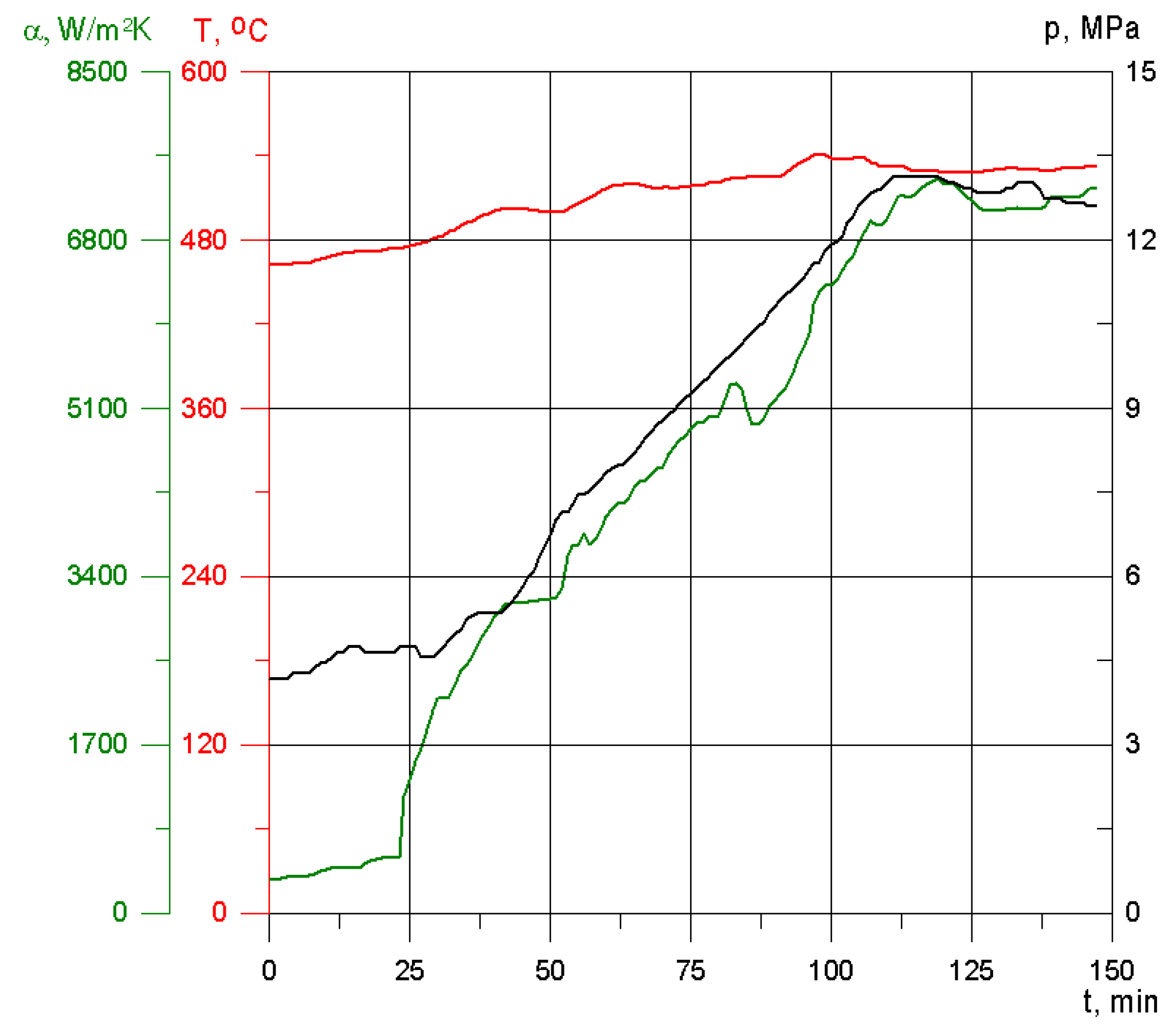
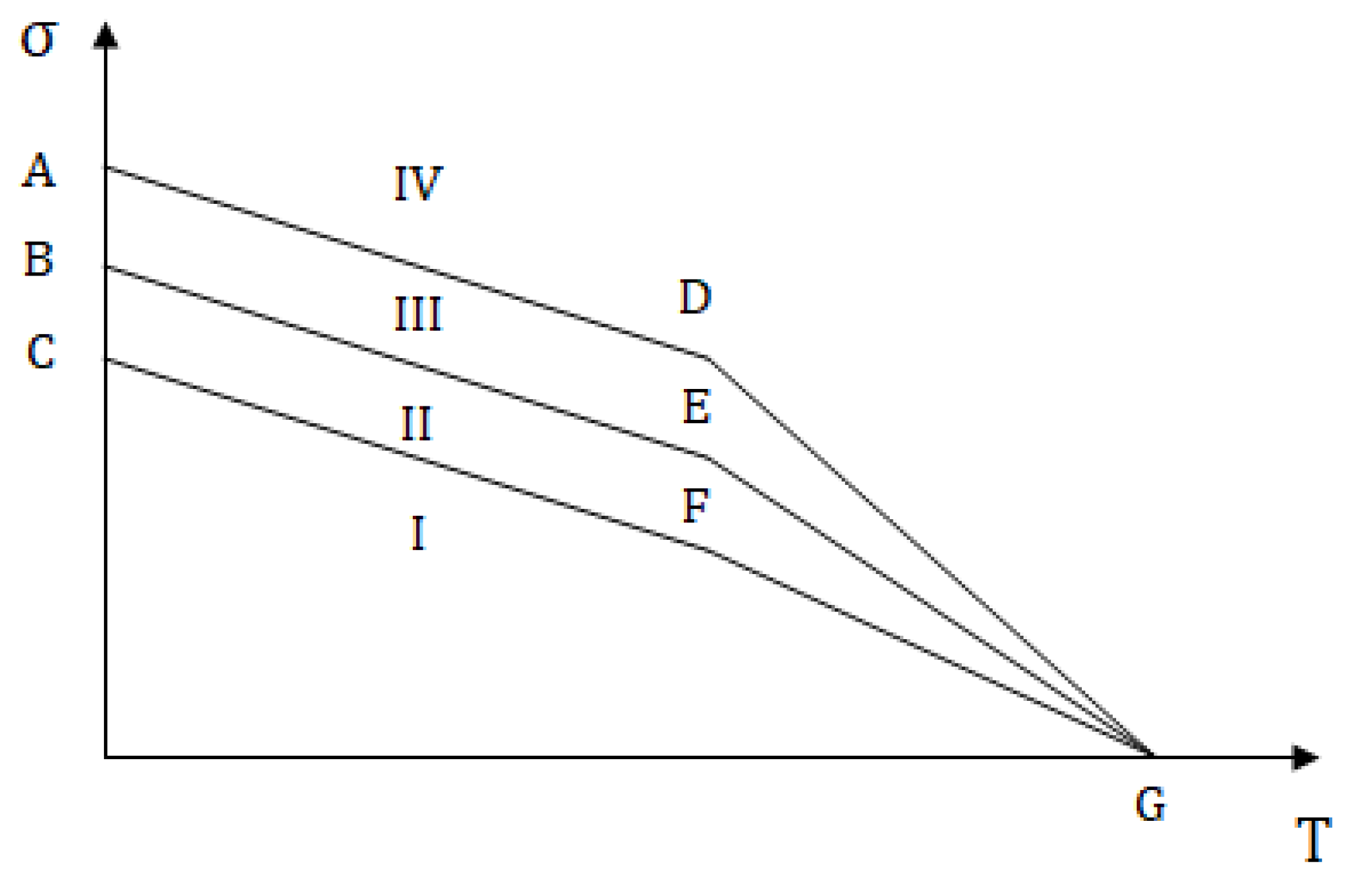
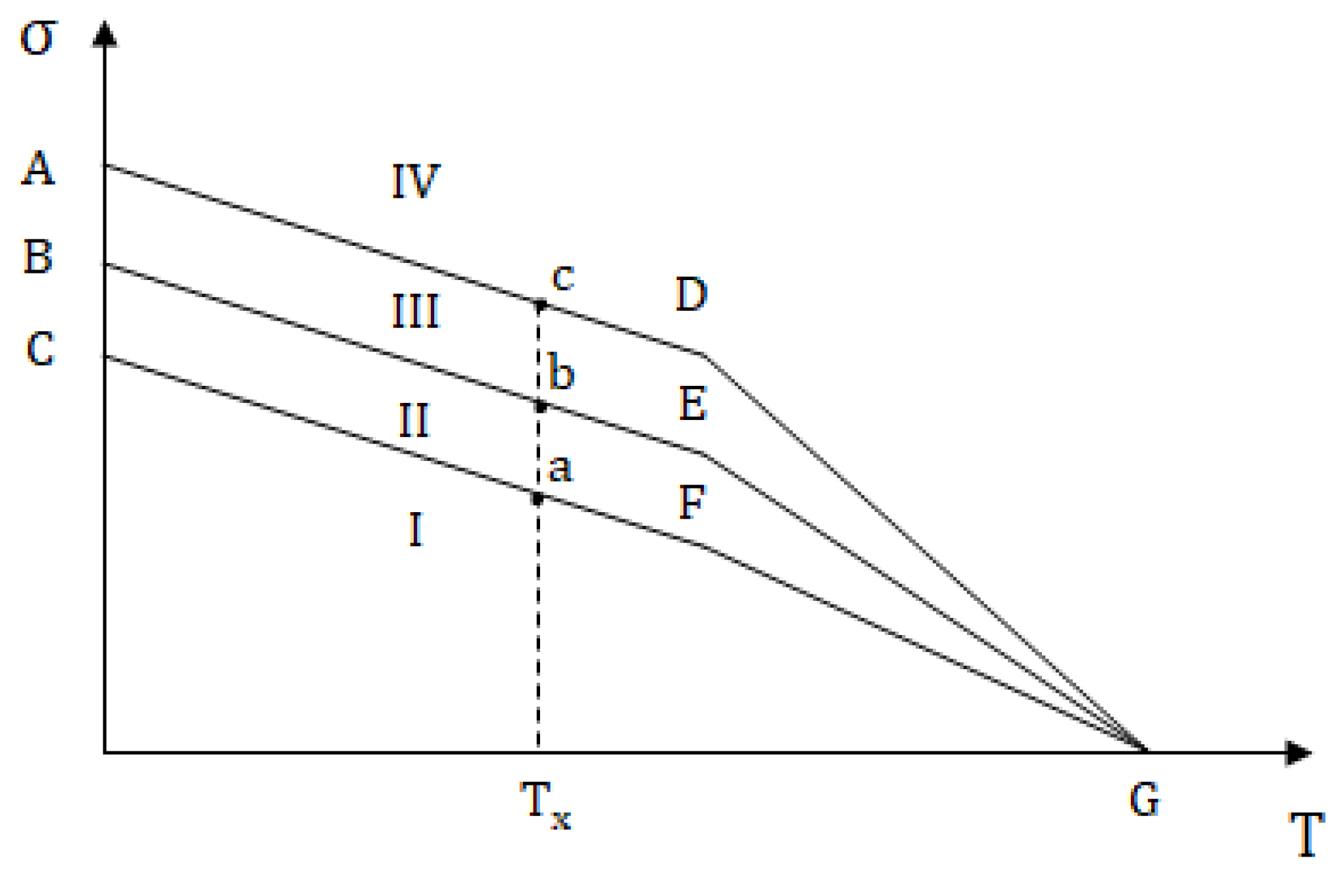
4.2. Turbine Cut-Off Valve
- Interval I: ,
- Interval II: .
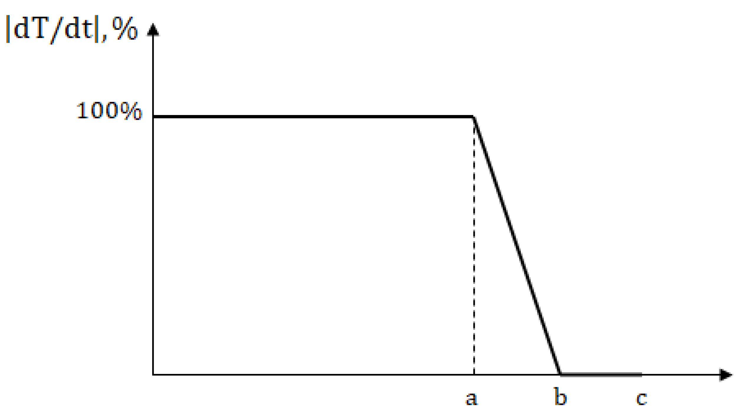
- Interval I:
- Interval II:
5. Controlling the Change in the Turbine Load Depending on the Stress Level
6. Conclusions
Author Contributions
Funding
Data Availability Statement
Conflicts of Interest
References
- Stoppato, A.; Mirandola, A.; Meneghetti, G.; Lo Casto, E. On the operation strategy of steam power plants working at variable load: Technical and economic issues. Energy 2012, 37, 228–236. [Google Scholar] [CrossRef]
- Rusin, A.; Bieniek, M.; Lipka, M. Assessment of the rise in the turbine operational risk due to increased cyclicity of power unit operation. Energy 2016, 96, 394–403. [Google Scholar] [CrossRef]
- Łukowicz, H.; Rusin, A. The impact of the control method of cyclic operation on the power unit efficiency and life. Energy 2018, 150, 565–574. [Google Scholar] [CrossRef]
- Tomala, M.; Rusin, A.; Wojaczek, A. Risk-Based Planning of Diagnostic Testing of Turbines Operating with Increased Flexibility. Energies 2020, 13, 3464. [Google Scholar] [CrossRef]
- Lausterer, G.K. On-line thermal stress monitoring using mathematical models. Control. Eng. Pract. 1997, 5, 85–90. [Google Scholar] [CrossRef]
- Taler, J.; Węglowski, B.; Zima, W.; Grądziel, S.; Zborowski, M. Analysis of Thermal Stresses in a Boiler Drum During Start-up. J. Press. Vessel. Technol. 1999, 121, 84–93. [Google Scholar] [CrossRef]
- Taler, J.; Dzierwa, P.; Taler, D.; Harchut, P. Optimization of the boiler start-up taking into account thermal stresses. Energy 2015, 92, 160–170. [Google Scholar] [CrossRef]
- Nowak, G.; Rusin, A.; Łukowicz, H.; Tomala, M. Improving the power unit operation flexibility by the turbine start-up optimization. Energy 2020, 198, 117303. [Google Scholar] [CrossRef]
- Dettori, S.; Maddaloni, A.; Colla, V.; Toscanelli, O.; Buciarelli, F.; Signorini, A.; Checcacci, D. Nonlinear model predictive control strategy for steam turbine rotor stress. Energy Procedia 2019, 158, 5653–5658. [Google Scholar] [CrossRef]
- Song, G.; Kim, B.; Chang, S. Fatigue life evaluation for turbine rotor using Green’s function. Procedia Eng. 2011, 10, 2292–2297. [Google Scholar] [CrossRef] [Green Version]
- Mukhopadhyay, N.K.; Dutta, B.K.; Kushwaha, H.S. On-line fatigue-creep monitoring system for high-temperature components of power plants. Int. J. Fatigue 2001, 23, 549–560. [Google Scholar] [CrossRef]
- Rusin, A.; Nowak, G.; Lipka, M. Practical algorithms for online thermal stress calculations and heating process control. J. Therm. Stresses 2014, 37, 1286–1301. [Google Scholar] [CrossRef]
- Nowak, G.; Rusin, A. Using the artificial neural network to control the steam turbine heating process. Appl. Therm. Eng. 2016, 108, 204–210. [Google Scholar] [CrossRef]
- Ko, H.O.; Jhung, M.J.; Choi, J.B. Development of Green’s function approach considering temperature-dependent material properties and its application. Nucl. Eng. Technol. 2014, 47, 101–108. [Google Scholar] [CrossRef] [Green Version]
- Zhang, H.L.; Liu, S.; Xie, D.; Xiong, Y.; Yu, Y.; Zhou, Y.; Guo, R. Online fatigue-monitoring models with consideration of temperature dependent properties and varying heat transfer coefficients. Sci. Technol. Nucl. Install. 2013, 2013. [Google Scholar] [CrossRef]
- Rouse, J.; Hyde, C. A comparison of simple methods to incorporate material temperature dependency in the Green’s function method for estimating transient thermal stresses in thick-walled power plant components. Materials 2016, 9, 26. [Google Scholar] [CrossRef] [Green Version]
- Koo, G.H.; Kwon, J.J.; Kim, W. Green’s function method with consideration of temperature dependent material properties for fatigue monitoring of nuclear power plants. Int. J. Press. Pip. 2009, 86, 187–195. [Google Scholar] [CrossRef]
- Łukowicz, H. Analysis Problems in Flow Calculations of Steam Turbines Applied in Diagnostics and Design. ZN Politech. Śląskiej S. Energetyka 2005, 143, 1–2. [Google Scholar]
- Rusin, A.; Łukowicz, H.; Kosman, W. Transient Temperature and Thermal Stresses in Turbine Components. In Encyclopedia of Thermal Stresses; Springer Science: Dordrecht, The Netherland, 2015. [Google Scholar]
- Chmielniak, T.; Kosman, G.; Łukowicz, H. Analysis of Mean Convective Heat Transfer Coefficients in Steam Turbine Valves. Trans. Inst. Fluid Flow Mach. 1994, 87, 25–40. [Google Scholar]
- Dirker, J.; Meyer, J.P. Convective Heat Transfer Coefficients in Concentric Annuli. Heat Transf. Eng. 2005, 26, 38–44. [Google Scholar] [CrossRef]


Publisher’s Note: MDPI stays neutral with regard to jurisdictional claims in published maps and institutional affiliations. |
© 2021 by the authors. Licensee MDPI, Basel, Switzerland. This article is an open access article distributed under the terms and conditions of the Creative Commons Attribution (CC BY) license (https://creativecommons.org/licenses/by/4.0/).
Share and Cite
Rusin, A.; Tomala, M.; Łukowicz, H.; Nowak, G.; Kosman, W. On-Line Control of Stresses in the Power Unit Pressure Elements Taking Account of Variable Heat Transfer Conditions. Energies 2021, 14, 4708. https://doi.org/10.3390/en14154708
Rusin A, Tomala M, Łukowicz H, Nowak G, Kosman W. On-Line Control of Stresses in the Power Unit Pressure Elements Taking Account of Variable Heat Transfer Conditions. Energies. 2021; 14(15):4708. https://doi.org/10.3390/en14154708
Chicago/Turabian StyleRusin, Andrzej, Martyna Tomala, Henryk Łukowicz, Grzegorz Nowak, and Wojciech Kosman. 2021. "On-Line Control of Stresses in the Power Unit Pressure Elements Taking Account of Variable Heat Transfer Conditions" Energies 14, no. 15: 4708. https://doi.org/10.3390/en14154708