Dynamics Analysis Using Koopman Mode Decomposition of a Microgrid Including Virtual Synchronous Generator-Based Inverters

Abstract

In the field of microgrids (MGs), steady-state power imbalances and frequency/voltage fluctuations in the transient state have been gaining prominence owing to the advancing distributed energy resources (DERs) connected to MGs via grid-connected inverters. Because a stable, safe power supply and demand must be maintained, accurate analyses of power system dynamics are crucial. However, the natural frequency components present in the dynamics make analyses complex. The nonlinearity and confidentiality of grid-connected inverters also hinder controllability. The MG considered in this study consisted of a synchronous generator (the main power source) and multiple grid-connected inverters with storage batteries and virtual synchronous generator (VSG) control. Although smart inverter controls such as VSG contribute to system stabilization, they induce system nonlinearity. Therefore, Koopman mode decomposition (KMD) was utilized in this study for consideration as a future method of data-driven analysis of the measured frequencies and voltages, and a frequency response analysis of the power system dynamics was performed. The Koopman operator is a linear operator on an infinite dimensional space, whereas the original dynamics is a nonlinear map on a finite state space. In other words, the proposed method can precisely analyze all the dynamics of the power system, which involve the complex nonlinearities caused by VSGs.

1. Introduction

To achieve environmental friendliness and sustainability, various types of power sources are freely connected to power systems. Moreover, distributed energy resources (DERs) such as batteries must be connected to use renewable energy, thereby avoiding fossil fuel depletion, and to shield the power system from accidental power outages caused by natural disasters such as hurricanes and earthquakes. It is a major challenge to maintain system stability in microgrids (MGs), which include small DERs with autonomous power, unlike traditional power systems, which are powered by large synchronous generators (SGs) with large inertial forces and short-circuit ratios (SCRs). Because the SCR is determined by the system voltage, impedance, and power supply capacity, the SCR of a small DER connected to a low-voltage distribution system cannot be increased. Furthermore, to protect the equipment from accidental overcurrent or overvoltage, a conventional grid-connected inverter, which cannot have inertial force, is controlled to respond immediately.

Numerous studies on new methods of grid-connected inverter control are underway to overcome the problem of inertial force. In particular, virtual synchronous generator (VSG) control of grid-connected inverters is attracting attention. VSG control can contribute to frequency stabilization by using battery energy as the inertial force of the SG [1,2,3,4]. VSG inverter controls, also called “smart inverters,” were proposed at approximately the same time [1,2]. In the corresponding methods, the inertial control and voltage control of an SG supplement the conventional current control method installed in power conditioning systems. In contrast, Zhong et al. [3] based their research on the voltage control method and faithfully reproduced Park’s generator theory with a controller. Meanwhile, Hirase et al. [4] analyzed the transient response of the VSG control and frequency response.

The grid-connected inverters that are used when DERs are connected to a grid are required to comply with the grid codes, although the methods of achieving compliance differ by manufacturer and are not disclosed. Because it is more complicated to analyze a system that includes a large number of black-boxed smart inverters, as described above, research is also underway to make the grid code applied to such inverters necessary and sufficient [5,6,7,8]. In [5,6], the correlations among frequency fluctuation, time, and control parameters were quantified by presenting analyses of the transient response of a VSG inverter based on the generator mechanism. Hashimoto et al. [7] presented a test method for obtaining comprehensive indices of the characteristics of various residential single-phase photovoltaic (PV) inverters. In addition, the use of power/control hardware-in-the-loop (PHIL/CHIL) is being actively promoted for the testing of various power supplies and interoperable controllers [8]. Nevertheless, both types of analyses model and approximate the system dynamics within the controller and simulate its behavior.

In recent years, power semiconductor materials such as silicon carbide (SiC) and gallium nitride (GaN), and communication technologies such as the fifth-generation (5G) mobile communication system, have improved dramatically, and breakthroughs have also occurred in power system development. Previously, communication delays occurring in the supervisory control and data acquisition (SCADA) were fatal for controls requiring high speed, such as transient response controls. However, we can now analyze and control data measured in real time using the aforementioned innovative technologies. This method is called the “data-driven approach” [9,10,11,12,13,14]; it is characterized by calculation of the dynamics to be analyzed and controlled based on the acquired data. Park et al. [9] estimated the load consumption in a building by modeling based on an unsupervised learning method, as well as the demand response. Similarly, Gorjão et al. [10] calculated a stochastic model from the obtained data (market rules, consumer behavior, etc.) and performed a frequency analysis. Xinhui et al. [11] improved the calculation speed of the above methods by estimating the state from past data. Li et al. [12] estimated a dynamic model using synchronous phase measurements, whereas Almunif et al. [13] identified low-dimensional eigenvalues of power systems and enhanced noise immunity. Liu et al. [14] improved the robustness and calculation speed of the power system by evaluating the static voltage stabilization margin (VSM).

The key points of the preceding discussion can be summarized as follows. First, the analysis of a power system is complicated when numerous DERs are connected to it. Next, DERs are connected via grid-connected inverters, and conventional inverters lack stability owing to their responsiveness. Meanwhile, sophisticated autonomous controls for system stabilization, such as the VSG controls in smart inverters, are not publicly available. Nevertheless, thanks to 5G technology, the development of data-driven system analysis and controls that attempt to simultaneously perform system measurement and control is progressing. However, the dynamics of complex power systems are high-order, and the spectral characteristics of the dynamics can be compromised by reducing the order and approximating the dynamics in a data-driven approach.

To handle the high-order and nonlinear dynamics, a dynamic analysis method that uses the spectral characteristics of the linear Koopman operator (KO) has been proposed [15]. Although the introduction of the KO dates back to 1931 [16], the computational technology of the time hindered its application in industry. Dynamic mode decomposition (DMD) using the KO is called Koopman mode decomposition (KMD), and it calculates the eigenvalues (KEs) and modes (KMs) of KOs using empirical values obtained from nonlinear dynamics, even if the dynamic operator itself is not clear [17]. In recent years, increasingly many mathematical studies focusing on the spectral characteristics of the KO have appeared [17,18,19,20,21,22,23,24,25,26]. Cho and Yamazaki [18] classifies the properties of a composition operator, which is another name of KO. Williams et al. [19] presented a data-driven method for approximating the leading KEs and KMs. Surana [20] demonstrated forecasting and anomaly detection using nonlinear dynamic generative modeling of a time series based on the KO. Meanwhile, Lange et al. [21] described a spectral decomposition method that is applicable to nonlinear systems. The Fourier transform applied to a linear system was extended using KO, without assuming periodicity, thereby facilitating long-term predictions based on data measured at arbitrary sampling intervals. Arbabi and Mezic [22] demonstrated the spectral decomposition of KO in the DMD by assuming that the underlying dynamical system was ergodic. They also showed that the singular value decomposition, which is central to most DMD algorithms, converges to the appropriate orthogonal decomposition of the observable. Takeishi et al. [23] and Sinha et al. [24] described a KO approximation method used for observables with large measurement noise. Takeishi et al. [25] also introduced an application of KMD to a neural network and showed that KO has an invariant subspace even when an observable that spans it is not available. Further, Črnjarić-Žic et al. [26] discussed the characteristics of the KEs and KMs for the stochastic KO in various types of linear random dynamical systems (RDS).

Because of the high level of accuracy of its nonlinear dynamics estimations, the KO has been utilized for actual analyses. Among such analyses, those described in [27,28,29,30,31,32] are related to power systems. Susuki and Mezić [27] applied KMD to two major sets of actual accident data (the 2011 Arizona-Southern California power outage and the 2006 European interconnection grid system failure) to detect unstable power flow patterns. Susuki et al. [28] also described coherency identification regarding the swing of SGs that interfere with each other. Meanwhile, Jlassi et al. [29] determined the minimum number of calculations required for KMD convergence, and the results of the discrete Fourier transform (DFT) and KMD were compared to identify the nonlinear characteristics confirmed by KMD. Later, Korda et al. [30] introduced a method of combining KMD analysis results with model predictive control (MPC). Hernandez-Ortega and Messina [31] used KMD to improve the approximation accuracy when reducing the order of a nonlinear perturbation analysis model to an arbitrary order. Finally, Cassamo and van Wingerden [32] described a method of applying the KO to the aerodynamic analysis of a wind power generation system to reproduce a low-dimensional linear state-space model accurately, thereby reducing the design cost of the controller.

With the above research as a background, we focused on both the voltage stability and frequency stability of a power system in this study and attempted to extract the characteristics of their mutual interference using KMD. While prior literature [27,28] analyzes the steady-state power fluctuations of large-scale power systems in detail, this study focuses on the transient response in MGs including DERs and analyze the nonlinearity in transient response caused by their controls. The characteristic extraction results were visualized by widening the parameter range of the VSG control inverter. The test system was an Institution of Electrical and Electronic Engineering (IEEE) nine-bus model that included a main power supply and two distributed power supplies, which were inverters with storage batteries. The inverters were controlled by VSG control. The transient responses and DFTs of the system frequencies and terminal voltages were also calculated and compared with the results of KMD, thereby confirming the effect of cross-interference in the VSG control that appears only in KMD. The remainder of this paper is structured as follows. Section 2 reviews the KO and KMD. Section 3 explains the simulation test system used in this study. Section 4 presents analyses of the frequency response of the KMs when applying KMD. Finally, Section 5 summarizes the study.

2. Theory of the Koopman Operator (KO) and Koopman Mode Decomposition (KMD)

We briefly review the concept of the KO and KMD calculation method, which yields approximate values of the KEs and KMs. Further details are presented in [19,27,28].

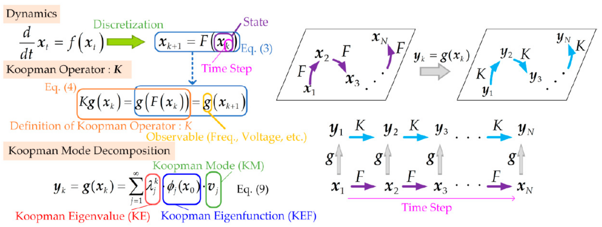
2.1. Koopman Operator (KO)

Let $M$ be a state space and $f:M\to M$ a vector-valued function. Equation (1) presents the dynamics of the state variable vector $x_t\in M$, and Equation (2) presents the dynamics at time $t\in {ℝ}^{+}$ with the initial time $t_0\in {ℝ}^{+}$. Equation (3) is a transformation of the integral-difference equation (Equation (2)) of a continuous system into a discrete system. In a power system with various types of generators, $F_t$ is typically nonlinear.

$$\frac{d}{dt}{x}_t=f\left(x_t\right),$$

(1)

$$F_t\left(x_{t_0}\right)=x_{t_0+t}=x_{t_0}+{\displaystyle {\int }_{t_0}^{t_0+t}f\left(x_{\tau }\right)}d\tau ,$$

(2)

$$x_{k+1}=F(x_k), \mathrm{where} \mathrm{we} \mathrm{define} F:=F_1.$$

(3)

To define the concept of the KO, let $G$ be the space of the observable. The linear operator $K$ is defined on $G$, which maps the observable $g:M\to ℂ$ to the new observable, as shown in Equation (4). As evident in the power system, any element, such as the frequency, phase, or voltage, at the terminal of each generator can be selected.

$$Kg:=g\circ F (g\in G).$$

(4)

The observables are obtained in a discrete-time system, and the observable $g(x_t)$ with dynamics $F$ can be rewritten as Equation (5) from Equations (3) and (4):

$$g\left(x_k\right)=g\left(F(x_{k-1})\right)=Kg\left(x_{k-1}\right)=K^{2}g\left(x_{k-2}\right)=\cdots =K^{k}g\left(x_0\right).$$

(5)

$K^k$ is an operator that represents the time evolution of the observable $g$ up to time $t$, and it is referred to as the KO. The KO $K$ is a linear operator on an infinite dimensional space $G$ even though the original dynamics $F$ are a nonlinear map on a finite state space $M$. The expression of nonlinear dynamics using linear operators could be employed to analyze the factors contributing to system instability that are attributable nonlinear dynamics without linear approximation. In addition, it is useful to divert control library assets that are commonly applied to linear dynamics.

2.2. Koopman Mode Decomposition

The KO $K$ has eigenfunctions ${\varphi }_j\in G$ that correspond to eigenvalues ${\lambda }_j\in ℂ$ that satisfy Equation (6). ${\lambda }_j$ and ${\varphi }_j$ are called Koopman eigenvalues (KEs) and Koopman eigenfunctions (KEFs), respectively:

$$K{\varphi }_j={\lambda }_j{\varphi }_j, j=1,2,\cdots .$$

(6)

Consider the m-dimensional vector $g\in M^m$ of the observables, that is $g={[g_1,\cdots ,g_m]}^T$, where the superscript $T$ denotes the transpose. If ${\varphi }_j\in G$, $j=1,2,\cdots$ span the whole $G$, then any observable $g_i\in G$ can be represented by the Fourier series as follows:

$$g_i={\displaystyle \sum _{j=1}^{\infty }{\varphi }_j}{v}_{ij}, i=1,2,\cdots ,m.$$

(7)

Using Equations (3), (4) and (6), the time evolution of the i-th observable $g_i(x_k)$ at the time step $k$ derived from (7) can be expressed as Equation (8). Equation (9) demonstrates the decomposition of the observable vector $g$ into an infinite number of oscillation modes, which is called KMD. Each oscillation mode is represented by the product of KEs, KEFs, and the complex vectors $v_j={\left[v_{1j},v_{2j},\cdots ,v_{mj}\right]}^T$, which are called Koopman modes (KMs). Figure 1 illustrates the concepts of the KO and KMD.

$$\begin{array}{ll}{g}_i(x_k)& ={\displaystyle \sum _{j=1}^{\infty }{\varphi }_j}(x_k)v_{ij}\\ & ={\displaystyle \sum _{j=1}^{\infty }{\lambda }_j{}^k{\varphi }_j}(x_0)v_{ij},\end{array}$$

(8)

where x₀ is the initial state variable vector.

$y_k:=g(x_k)\in {ℂ}^m$ is defined as follows:

$$y_k:=g(x_k)={\displaystyle \sum _{j=1}^{\infty }{\lambda }_j^k\cdot {\varphi }_j(}{x}_0)\cdot v_j.$$

(9)

2.3. Arnoldi Algorithm

It is difficult to know the nonlinear dynamics $F$ in advance, because DERs are repeatedly added and disconnected at arbitrary times. That is, it may not be possible to obtain the theoretical formula for KMD, because the KE and KEFs generally cannot be obtained. It is thus necessary to acquire the observables with minimal delay and to identify the system utilizing them. In this study, the Arnoldi-type algorithm was applied so that both the KEs and KMs could be calculated from time series observables without knowing the dynamics $F$ or KO $K$.

$N+1$ is a finite integer indicating the number of time samples, and we consider the observation of time series data $\left\{g(x_0),\cdots ,g(x_N)\right\}$. The coefficients $c_j$ that satisfy Equation (10) can be calculated when the vector $r$ is orthogonal to the space spanned by $\left\{g(x_0),\cdots ,g(x_{N-1})\right\}$. In particular, from the inner-product $〈r,g(x_j)〉=0$ ($j=0,\cdots ,N-1$), $c_j$ can be obtained by solving Equation (11).

$$r=g(x_N)-{\displaystyle \sum _{j=0}^{N-1}{c}_{j}g(x_j)},$$

(10)

$$\left[\begin{array}{ccc}〈g(x_0),g(x_0)〉& \cdots & 〈g(x_{N-1}),g(x_0)〉\\ ⋮& \ddots & ⋮\\ 〈g(x_0),g(x_{N-1})〉& \cdots & 〈g(x_{N-1}),g(x_{N-1})〉\end{array}\right]\left[\begin{array}{c}{c}_0\\ ⋮\\ c_{N-1}\end{array}\right]=\left[\begin{array}{c}〈g(x_N),g(x_0)〉\\ ⋮\\ 〈g(x_N),g(x_{N-1})〉\end{array}\right].$$

(11)

Let $A\in {ℝ}^{N\times N}$ and $b,c\in {ℝ}^N$ be as in Equation (11); that is, $Ac:=b$ holds, and by using the Moore Penrose pseudo-inverse matrix $A^{+}$, $A^{+}Ac=A^{+}b$ is satisfied. If $A$ is regular, $c$ can be calculated from $c=A^{-1}b$, and even if it is not, $‖Ac-b‖$ can be minimized by setting $c=A^{+}b$. The $N$ eigenvalues of the companion matrix $C\in {ℝ}^{N\times N}$ defined by $c_0,c_1,\cdots c_{N-1}\in ℝ$ (Equation (12)) are empirical Ritz values (${\tilde{\lambda }}_j$, $j=0,\cdots ,N-1$) and can be considered equivalent to KEs (${\lambda }_j$, $j=0,\cdots ,N-1$).

$$C=\left[\begin{array}{ccccc}0& 0& \cdots & 0& c_0\\ 1& 0& \cdots & 0& c_1\\ 0& 1& \cdots & 0& c_2\\ ⋮& ⋮& \ddots & ⋮& ⋮\\ 0& 0& \cdots & 1& c_{N-1}\end{array}\right].$$

(12)

When the matrix $V=\left[g(x_0)\cdots g(x_{N-1})\right]U^{-1}\in {ℂ}^{N\times N}$ is obtained by using Equations (13) and (14) holds. Each column ${\tilde{v}}_j$ of $U$ corresponds to ${\varphi }_j(x_0)v_j$ (i.e., the KEFs and KMs) in Equation (9), where $U$ represents the Vandermode matrix and ${\tilde{\lambda }}_j$ are the empirical Ritz values:

$$U=\left[\begin{array}{ccccc}1& {\tilde{\lambda }}_1& {\tilde{\lambda }}_1{}^2& \cdots & {\tilde{\lambda }}_1{}^{N-1}\\ 1& {\tilde{\lambda }}_2& {\tilde{\lambda }}_2{}^2& \cdots & {\tilde{\lambda }}_2{}^{N-1}\\ ⋮& ⋮& ⋮& \ddots & ⋮\\ 1& {\tilde{\lambda }}_N& {\tilde{\lambda }}_N{}^2& \cdots & {\tilde{\lambda }}_N{}^{N-1}\end{array}\right],$$

(13)

$$\left\{\begin{array}{l}g\left(x_k\right)={\displaystyle \sum _{j=0}^{N-1}{\tilde{\lambda }}_j{}^k{\tilde{v}}_j}\hspace{0.17em}\hspace{0.17em}\hspace{0.17em}\hspace{0.17em}\hspace{0.17em}\hspace{0.17em}(k=0,\cdots N-1)\\ g\left(x_N\right)={\displaystyle \sum _{j=0}^{N-1}{\tilde{\lambda }}_j{}^N{\tilde{v}}_j}+r\end{array}\right..$$

(14)

Because the differences between the empirical Ritz values and true values and between the finite and infinite series are small in the power system investigated in this study, we do not discuss how they differ here and rewrite ${\tilde{\lambda }}_j$ and ${\tilde{v}}_j$ as ${\lambda }_j$ and $v_j$.

3. Transient Responses of Power Systems

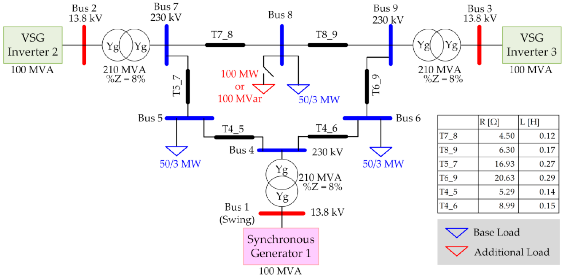
3.1. IEEE Nine-Bus Model Test System

In this study, we considered the IEEE nine-bus model (three-machine system) (Figure 2). One primary power supply was assumed to be a SG, and the other two generators were assumed to be distributed power sources of inverters with batteries which were equipped with the same VSG control. In the simulation tests, the SG model was that of the standard synchronous machine installed in the simulator. Figure 2 shows the rated capacities and voltages of the generators, bus voltages, line impedance, transformer capacities, and impedance. The total base load of 100 MVA was evenly distributed in the three locations of Buses 5, 6, and 8, and the simulation started with all the power being supplied from the main power supply (SG). A load of 100 MVA was added to Bus 8 in a stepwise manner, and the system fluctuation was analyzed immediately after adding the load. By adjusting the set point of the SG, the frequency and voltage just before the load was added were set to the rated values of 50 Hz and 13.8 kV. In the standard tests, the equipment constants and control parameters of all the generators were set to be nearly identical. In the other tests, the VSG control parameter was increased or decreased for comparative purposes. The main objective of this study was to investigate the instability caused by the interference between DERs (inverters) and the nonlinearity due to the interference of the control loop in each power supply.

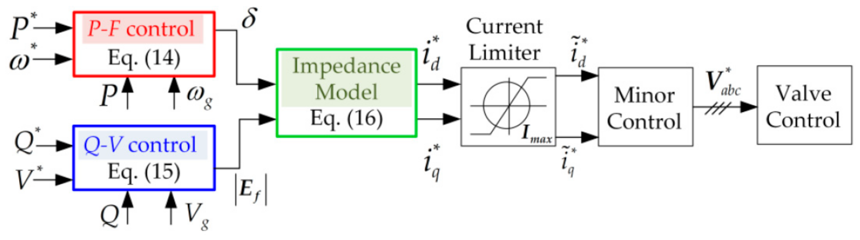
3.2. Virtual Synchronous Generator Control Model

Figure 3 shows a block diagram of VSG control. A Kawasaki VSG [2,4] was used in this study. The generator phase difference angle $\delta$ [rad] was calculated from Equation (15), which corresponds to the block enclosed by the red rectangle in Figure 3. $s$ denotes the Laplace operator. $P^{*}$ [pu] and $P$ [pu] denote the reference and feedback values of the active power, respectively. ${\omega }^{*}$ [pu] and ${\omega }_g$ [pu] are respectively the reference and feedback values of the angular frequency calculated at the output terminal of the VSG inverter. $K_{PF}$ [pu/pu] is the droop coefficient of the frequency (${\omega }_g$) with respect to $P$. The time constant $T_{PF}$ [s] is given by $T_{PF}=M{K}_{PF}$, where $M$ [s] is the unit inertia constant, and the first-order lag transfer function $K_{PF}/(1+s{T}_{PF})$ in Equation (14) represents the swing equation. A conventional swing equation is a higher-order equation (degree 2 or higher) because it includes the governor delay time and unit inertia constant. Conversely, the swing equation of the Kawasaki VSG becomes linear when the governor delay time, which is the characteristic of the Kawasaki VSG that is the easiest to adjust, is set to 0. The magnitude of the generator (induced) voltage vector $\left|E_f\right|$ [pu] is given by Equation (16). $K_{QV}$ [pu/pu] is the droop coefficient associated with the reactive power $Q$ [pu], and the magnitude of the terminal (inverter) voltage vector is $V_g=\left|V_g\right|$ [pu]. $Q^{*}$ [pu] and $V^{*}$ [pu] are the command values to $Q$ and $V_g$, respectively. $T_{QV}$ [s] is the measurement delay time of the terminal voltage, and the conventional proportional-integral (PI) compensator (for which the proportional and integral coefficients are $K_p$ and $K_i$, respectively) is used as the automatic voltage regulator (AVR). Equation (17) is the impedance model, which represents the relationship among $E_f$, $V_g$, and the command value vector $I^{*}$ of the inverter current. The impedance $r$ and $x$ [pu] constitute a pseudo-impedance set in the VSG control software and becomes dominant over the alternating current (AC) output filter impedance in low-frequency regions, such as commercial frequencies. The ratio of the virtual inductance $x$ to the virtual resistance $r$ was empirically set to $x=2r$.The current command value was limited to avoid overcurrent, and was input into the minor control, which was composed of current control. The pulse width modulation (PWM) command value ($V_{abc}^{*}$) output from the minor control was input into the valve control. Because these controls are conventional, detailed explanations are not included here.

$$\delta =\left(\left(P^{*}-P\right)\frac{K_{PF}}{1+s{T}_{PF}}+\left({\omega }^{*}-{\omega }_g\right)\right)\frac{1}{s}.$$

(15)

$$\left|E_f\right|=\left((Q^{*}-Q)\frac{K_{QV}}{1+s{T}_{QV}}+\left(V^{*}-\left|V_g\right|\right)\right)\left(K_p+\frac{K_i}{s}\right).$$

(16)

$$I^{*}=\left[\begin{array}{c}{i}_d^{*}\\ i_q^{*}\end{array}\right]=\frac{1}{r^2+x^2}\left[\begin{array}{cc}r& x\\ -x& r\end{array}\right]\left(E_f-V_g\right).$$

(17)

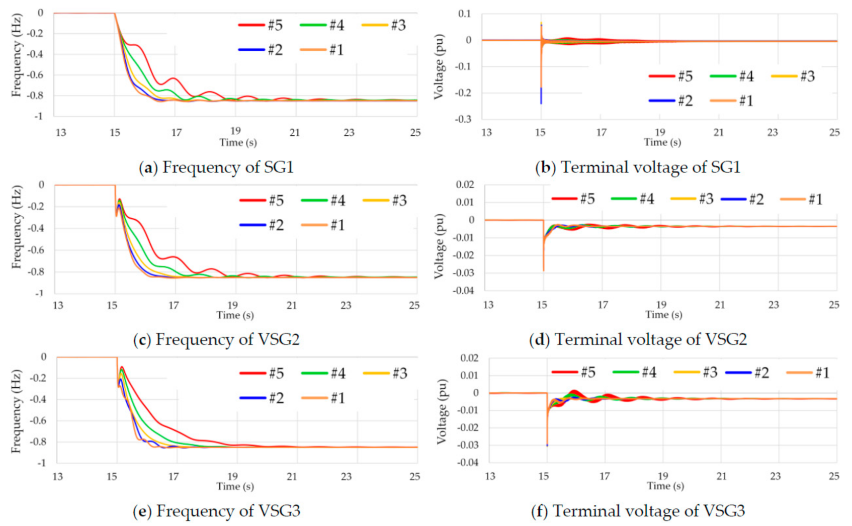
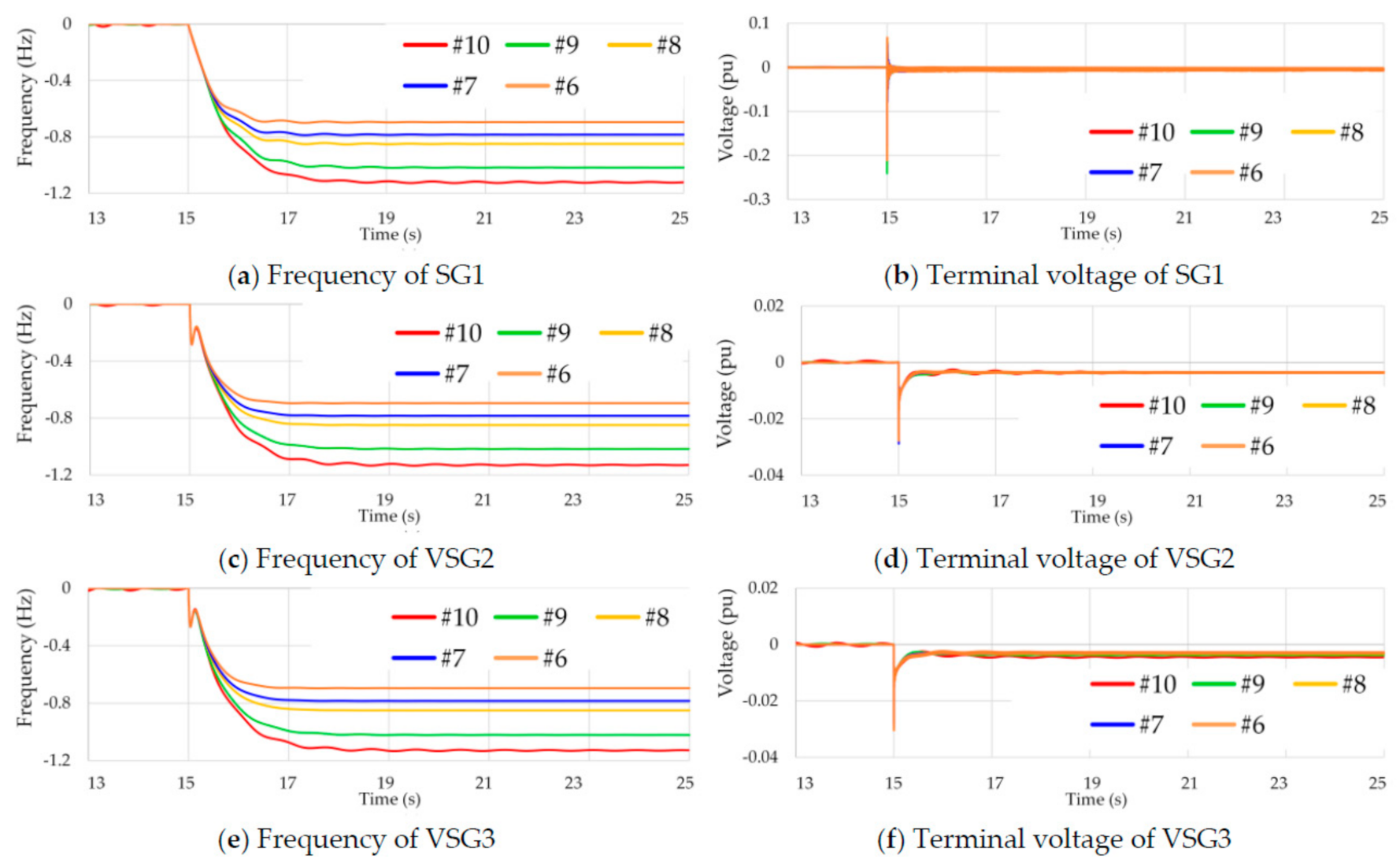
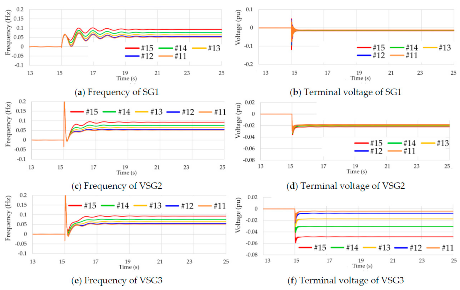
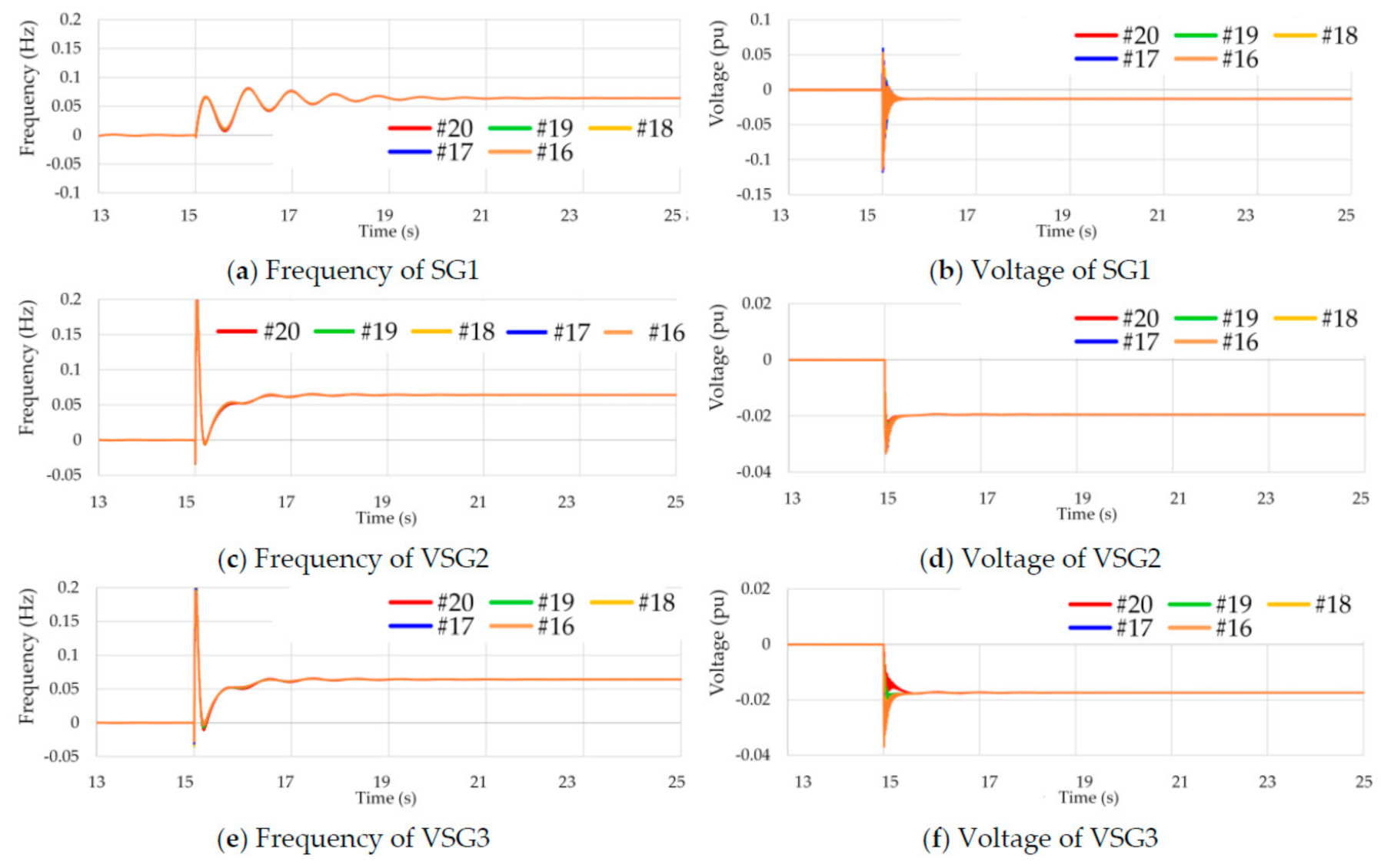
3.3. Simulation Tests

Numerical simulations were conducted using MATLAB/Simulink based on the connection diagram shown in Figure 2. The SG connected to Bus 1 and the VSGs connected to Buses 2 and 3 are referred to as SG1, VSG2, and VSG3, respectively. The parameters of each power supply ($K_{PF}$, $K_{QV}$, $M=T_{PF}/K_{PF}$, $T_{QV}$, etc.) are indicated by a subscript number $\_n$ ($n$ = 1, 2, 3), and

Table 1. Machine constants and control variables.

Machine	Test	$\mathit{P}-{\mathit{\omega }}_{\mathit{g}}$ Droop Constant	Unit Inertia Constant	$\mathit{Q}-{\mathit{V}}_{\mathit{g}}$ Droop Constant	$\mathbf{Measurement} \mathbf{Delay} \mathbf{Time} \mathbf{of} {\mathit{V}}_{\mathit{g}}$
		${\mathit{K}}_{\mathit{P}\mathit{F}\_\mathit{n}}$ (-)	${\mathit{M}}_{\_\mathit{n}}$ (s)	${\mathit{K}}_{\mathit{Q}\mathit{V}\_\mathit{n}}$ (-)	${\mathit{T}}_{\mathit{Q}\mathit{V}\_\mathit{n}}$ (s)
SG1	1–20	0.05	12	0.05	0.015
VSG2	1–20	0.05	12	0.05	0.015
VSG3	1	0.05	3	0.05	0.015
	2		6
	3		12
	4		24
	5		48
	6	0.03	12	0.05	0.015
	7	0.04
	8	0.05
	9	0.1
	10	0.2
	11	0.05	12	0.01	0.015
	12			0.02
	13			0.05
	14			0.1
	15			0.2
	16	0.05	12	0.05	0.001
	17				0.005
	18				0.015
	19				0.5
	20				1.5

lists the parameters for the 20 tests. In the standard tests (3, 8, 13, 18), the VSG3 parameters are almost equivalent to those of the SG1 and VSG2. In all tests (1–20), $K_p$ and $K_i$ in the PI compensator of the AVR are 10 and 80, respectively. All analyses were conducted using unit capacitance with the rated capacitance of each power supply set to 100 MVA at 1 pu. In tests 1–10, an active load of 100 MW was added 15 s after the simulation onset. Similarly, in tests 11–20, a reactive load of 100 MVar was added.

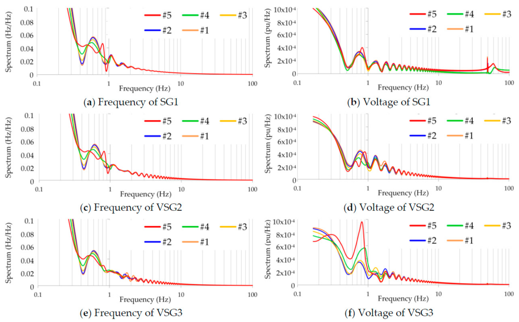
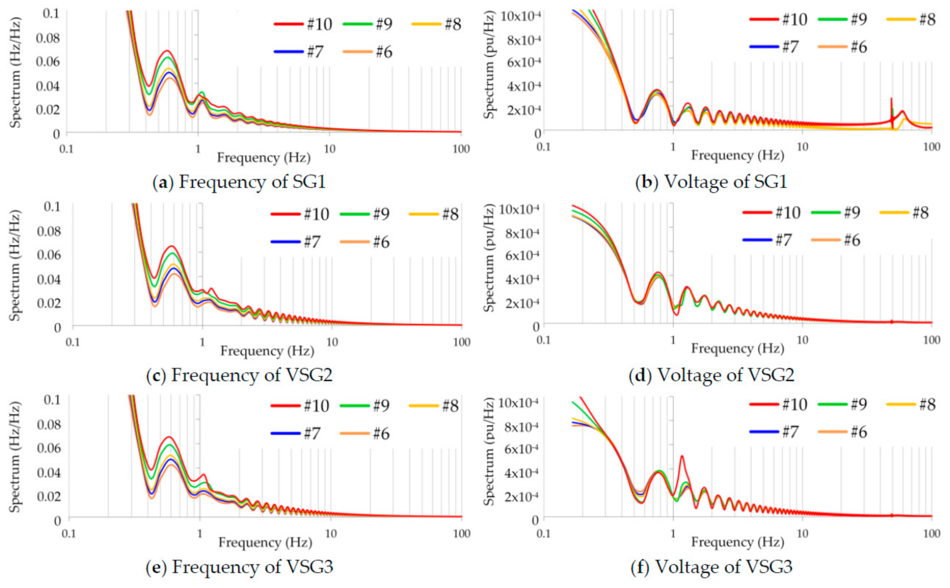
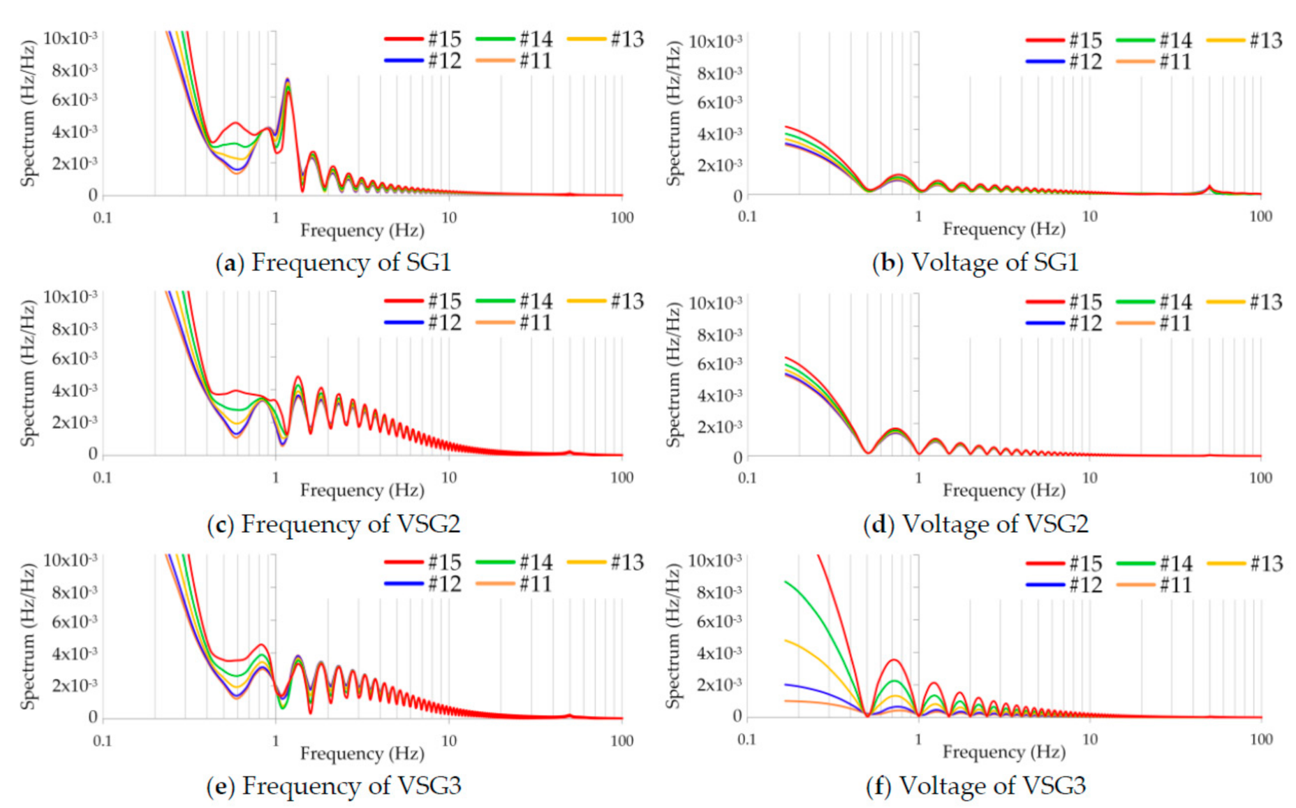
3.4. Transient and Frequency Response Analyses of Simulation Results

Figure 4, Figure 5, Figure 6 and Figure 7 show the simulated transient responses of the three power supplies obtained from tests 1–5, 6–10, 11–15, and 16–20, respectively. In each figure, (a–f) depict the results for SG1, VSG2, and VSG3, respectively. The left column (a,c,e) and the right column (b,d,f) present the results of frequencies and voltages measured at the terminal of each generator. Each observable (system frequency or terminal voltage of $N$ = 3000 points) was measured for 10 s from the onset time (15 s). A sample rate capable of measuring a rated system frequency of 50 Hz was required, and in this study, the sample rate was set to 250 Hz (sampling every 4 ms).

In tests 1–10, the system frequency changed according to the drooping characteristics owing to the addition of the active power load, and transient fluctuations due to the swing characteristics of the generators were confirmed. The swing characteristics of the generators reflect the relationship between the rotor angular velocities of the generators and the input/output torques. Thus, the addition of active power significantly affects the system frequency (a,c,e). However, the terminal voltage (b,d,f) is also affected. The high-frequency vibration of the terminal voltages and sudden fluctuations at 15 s are due to the load switch, the voltage controls, and the phase-locked loops (PLLs) in the VSG controls that were used to convert the control signals to a dq reference frame.

Conversely, the results of tests 11–20 reveal the voltage drooping characteristic resulting from the addition of reactive power. Unlike the system frequency, the terminal voltage differs for each measurement point. Therefore, the parameter differences among tests 11–20 considerably affected the terminal voltage of VSG3. Simultaneously, transient fluctuations and accelerations in the system frequencies due to the addition of reactive power were also confirmed. In tests 16–20, in which the measurement delay times of the terminal voltage were changed, there was almost no difference in the transient response results.

We applied DFT to the transient response simulation results (Figure 4, Figure 5, Figure 6 and Figure 7) to confirm the frequency characteristics. Figure 8, Figure 9, Figure 10 and Figure 11 show the results of DFT. The tests (1–20), columns (frequencies/voltages), and rows (SG1/VSG2/VSG3) were organized as shown in Figure 4, Figure 5, Figure 6 and Figure 7. DFT is another type of data-driven analysis that is similar to KMD and can be applied to systems with unknown dynamics. The difference is that KMD can be used to analyze systems that include both linear and nonlinear dynamics, whereas the DFT analyzes target systems that are linearized around the equilibrium point. That is, frequency response analysis using the DFT produces a large error around operating points with high nonlinearity.

As evident in the transient responses in Figure 4, Figure 5, Figure 6 and Figure 7, natural vibrations occurred in the low-frequency bands (0.1–10 Hz) and high-frequency bands near the system frequency of 50 Hz in most of the tests. The 50 Hz vibration could be confirmed by the terminal voltage of each generator and by the system frequencies in tests 11–20. Spectral peaks exist in the ranges of 0.5–0.8 Hz, 1.0–2.0 Hz, 2.0–10.0 Hz, and 50.0–60.0 Hz. Due to the sampling theorem and DFT calculation method, there are large errors in the bands exceeding 1/2 of the sampling frequency (250 Hz) and near 0 Hz.

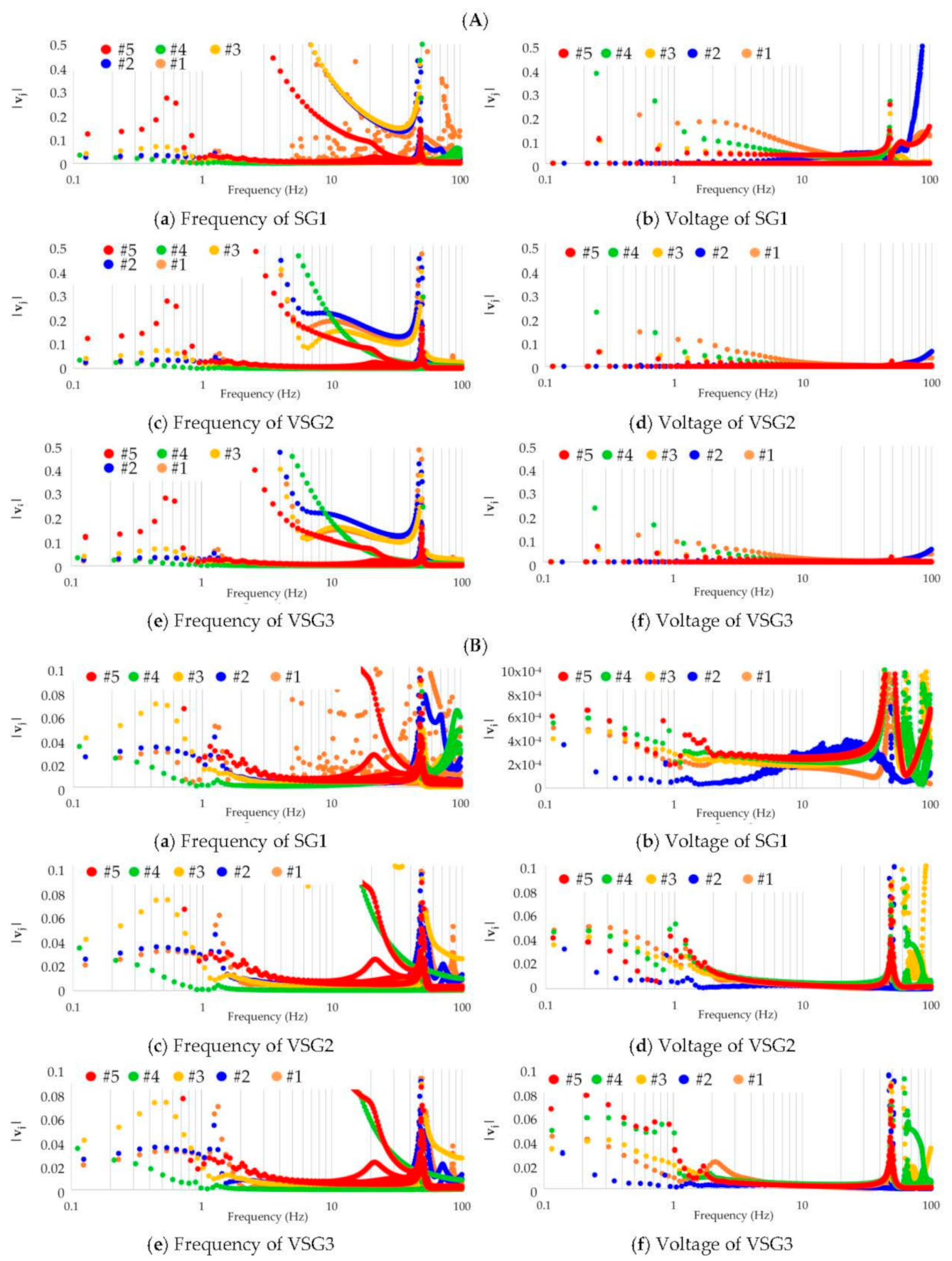
4. Koopman Mode Decompositions (KMDs) of Power System Observables

The system frequencies and terminal voltages (Figure 4, Figure 5, Figure 6 and Figure 7) measured at the output terminals of each power supply shown in Figure 2 were used as the observables $\left\{g(x_0),\cdots g(x_N)\right\}$, to which the Arnoldi algorithm described in Section 2.3 was applied to perform KMD. Subsequent analyses were performed assuming that the terminal voltages and system frequencies, which are the observables of the target power system, can be represented as shown in Equation (7). There were $N$ = 3000 measurement points (sampled every 4 ms for 12 s), and at each measurement point, the observable vector $g(x_j)$ ($0\le j\le N$) consisted of the components $g_1(x_j)$, $g_2(x_j)$, and $g_3(x_j)$, which were the measurement values of SG1, VSG2, and VSG3, respectively. Using Equations (13) and (14), we calculated KE ${\lambda }_j$, KM $v_j$, and the vibration frequency corresponding to each KE ${\lambda }_j$ at each measurement point ($0\le j\le N$). KEs ${\lambda }_j$ were complex scalars from which the arguments and vibration frequencies could be obtained, whereas KMs $v_j$ were complex vectors, where the KM components $v_{1j}$, $v_{2j}$, and $v_{3j}$ corresponded to $g_1(x_j)$, $g_2(x_j)$, and $g_3(x_j)$, respectively. Hereafter, by specifying “SG1”, “VSG2”, and “VSG3”, the subscripts 1, 2, and 3 will be omitted.

Figure 12, Figure 13, Figure 14 and Figure 15 illustrate the relationship between the vibration frequency and absolute value of KM components ($\left|v_j\right|$) of SG1, VSG2, and VSG3. The absolute values of the KMs represent the power spectrums in the frequency domain. Figure 12, Figure 13, Figure 14 and Figure 15 represent the frequency response analyses of the KMs calculated from the observables in tests 1–5, 6–10, 11–15, and 16–20, respectively. Remarkably, all the results exhibit the same characteristics: the absolute values of the KM components are divided into four different groups: Group 1 with the strong spectrum around 50 Hz, Group 2 with large spectrum in the band of approximately 3 Hz to 50 Hz, Group 3 with small spectrum in the band below approximately 5 Hz, and Group 4 with an intermediate spectrum in the band of approximately 1 Hz to 20 Hz. The different test results confirmed that the strong power spectrum in Group 1 is due to the observables measured by using PLLs in the VSGs. The results will be reported in another article. Figure 12B, Figure 13B, Figure 14B and Figure 15B show enlarged versions of the Group 3 shown in Figure 12A, Figure 13A, Figure 14A and Figure 15A.

In Figure 8a,c,e and Figure 12B(a,c,e), the characteristic natural frequencies in Group 3 are confirmed. Conversely, the KMs in Group 2 which are evident in Figure 12A(a,c,e) do not appear in Figure 8a,c,e. It was also confirmed in other tests that the power spectrum belonging to Group 2 was caused by the discontinuous changes of the observables due to the disturbance (load power addition) that occurred 15 s after the start of the simulation. As described in the previous section, the difference can be attributed to the fact that Figure 8 represents a system that is linearly approximated around the equilibrium point using the DFT, whereas in using KMD, Figure 12A,B represent the exactly equal (not approximate) system containing both linear and nonlinear elements.

In the controls of the SG and VSGs, the active power and system frequency exhibit a control loop with the same mechanism as in Equation (15), and the control loops between the reactive power and terminal voltage can be expressed by Equation (16). Furthermore, these control loops cross-interfere, as shown in Equation (17). In tests 1–20, the effects of the active power change on the terminal voltage and of the reactive power change on the system frequency, which correspond to the cross-interference, were also confirmed in Group 4. The cross-interference in Group 4 does not appear when using the DFT, but appears when using the KMD; this can be reasonably confirmed in the right columns (b,d,f) for tests 1–10 (Figure 12A and Figure 13A) and in the left columns (a,c,e) for tests 11–20 (Figure 14A and Figure 15A). These tendencies indicate that KMD can express the interference between cross-loops relatively clearly.

When the values of the main control parameters change, the amounts of vibration of the observables change slightly. In particular, for tests 16–20, no significant differences in the characteristics were observed within the range of parameters listed in Table 1. Furthermore, the system operated stably in all tests and did not collapse. In future research, it will be important to increase the parameter ranges and to perform a sensitivity analysis.

5. Conclusions

As the introduction of DERs using REs is accelerating, the analysis of power system dynamics is becoming increasingly complicated due to the following factors:

• The inverters that connect DERs to power grids comprise control loops for active/reactive power and frequency/voltage, and thus interfere with each other and exhibit nonlinear characteristics.
• The system stability contribution function for the synchronization power of a smart inverter is an interference factor between power supplies, and it is difficult to perform mathematical analyses for complicated connection configurations.
• Functions such as the fault ride-through (FRT) in the grid code require fast responsiveness from the grid-connected inverters, which depends on the detailed data acquisition and accurate numerical analysis of these operations.

Expectations have been increasing for data-driven analyses and control using data measured in real time. Therefore, to develop future data-driven control, we developed a new analysis method for the nonlinear dynamics of a power system using offline data. Frequencies and voltages, which are the observables of the main control loops, were obtained from simulation results obtained using MATLAB/Simulink and the IEEE nine-bus system. By applying linear KOs to these observables, we could analyze the nonlinear dynamics of the power system. The simulation system included two VSG inverters, which are classified as smart inverters, and one conventional synchronous generator as the main power source. The vibration frequencies were calculated from the KEs, and the frequency responses were confirmed through comparison with the DFT, which is a conventional analysis method that linearly approximates a system. The following conclusions are drawn based on this comparison:

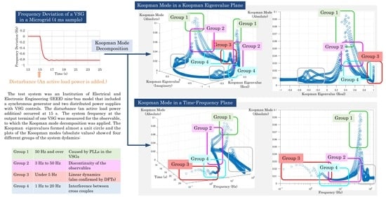
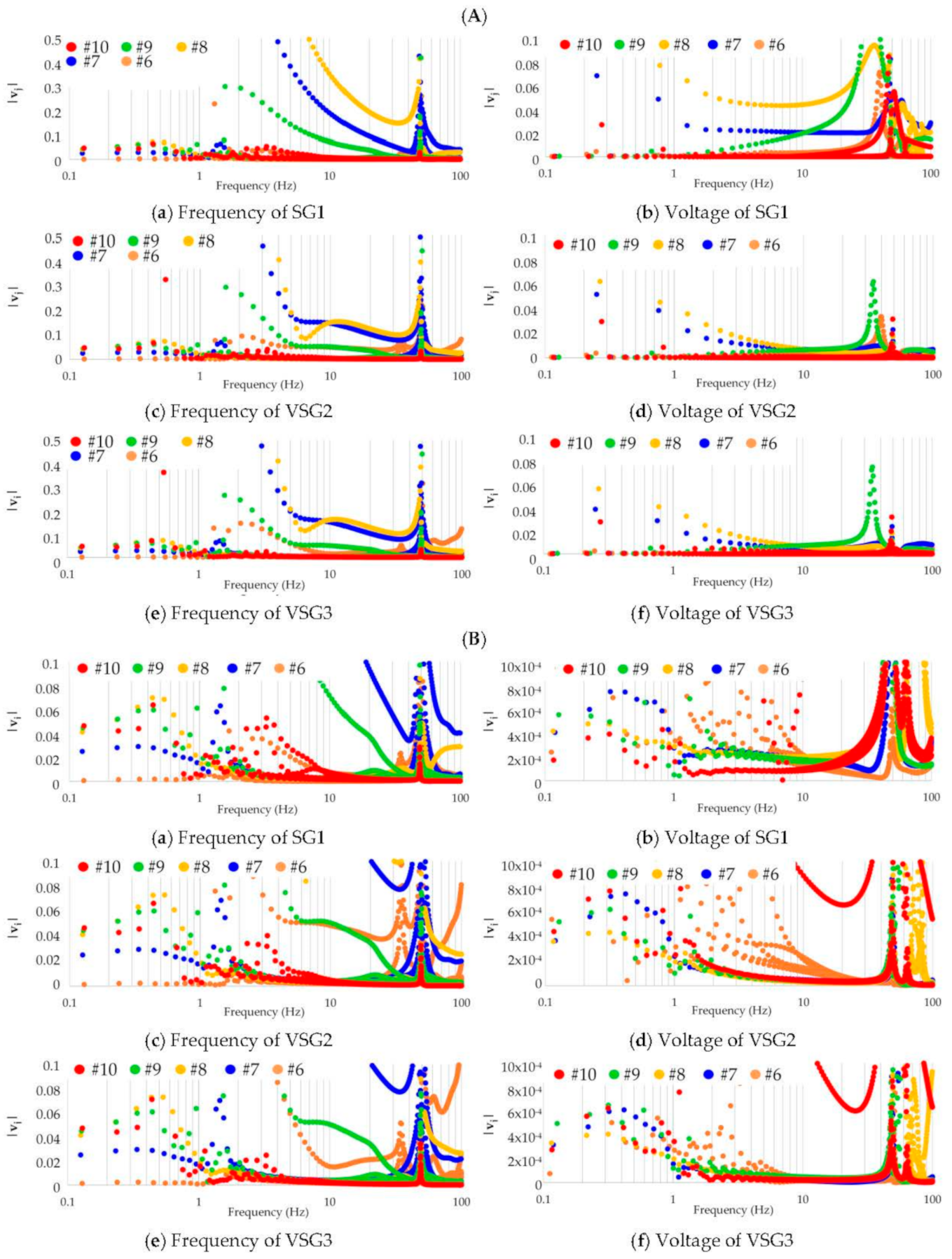
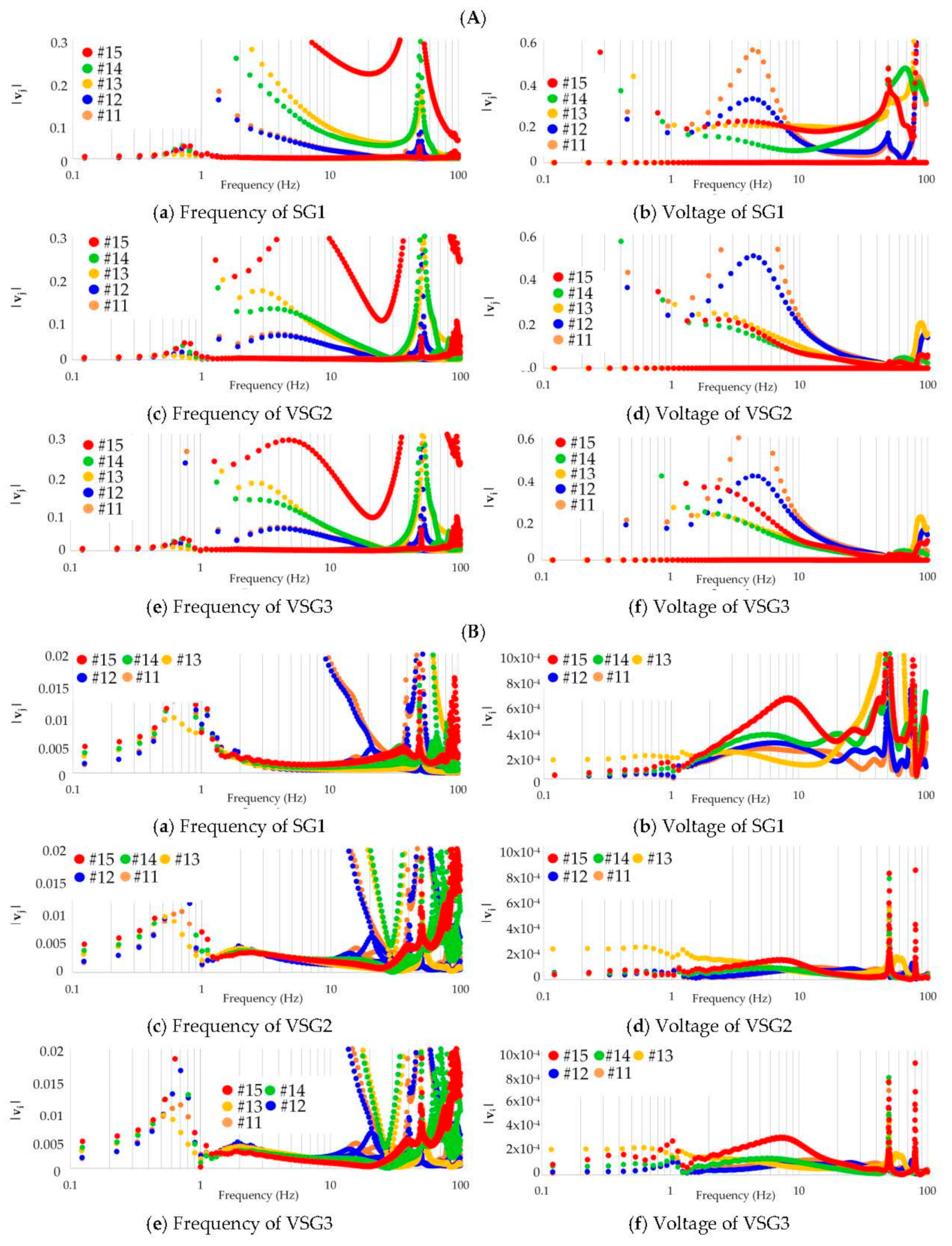
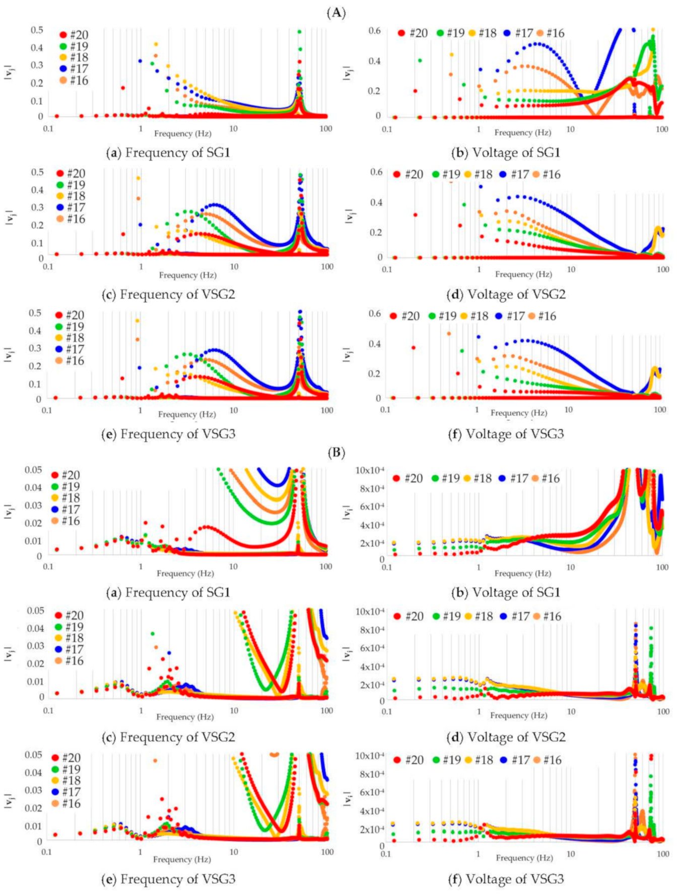
• The KMs calculated by using the Arnoldi algorithm in this study are approximations of the eigenfunctions of the KO. That is, when a system is series-expanded using the KEs and KEFs of the KO as the base, there are series terms represented by specific KEs and KEFs.
• Even if the frequency bands of the KEs are almost identical, the absolute values of the KM components tend to be divided into large and small groups. The absolute values of both differ by several orders of magnitude.
• The results obtained from the KMD method have KMs with large absolute values that cannot be confirmed by the DFT. Such power spectrum that does not appear in the DFT but appears only in the KMD can be considered to represent the nonlinearity in the dynamics. The simulation results indicate the power spectrum contained in the observables (frequency and voltage) that fluctuate discontinuously when the load power added.
• The AC power system is generally controlled in the dq reference frame. Therefore, the cross-couple effect due to the asymmetric term, which causes interference between the d-axis and q-axis control, must be determined. Although it is generally difficult to formulate the nonlinearity in the dynamics and analyze the control crossloops, KMD can clearly reveal these effects in the frequency bands at particular KEs. In the simulation tests of this study, it was confirmed that changes in active power affect not only system frequency but also terminal voltage by changing the control parameters of the inverter. Similarly, changes of the reactive power effect the system frequency as well as the terminal voltage.

When KMD is utilized in a power system, it can be applied for fault prediction and control stability by focusing on new phenomena that are not addressed by conventional approximation methods. However, the following tasks remain:

• Confirmation of how KMs with large absolute values behave in actual systems;
• Indexing of the magnitudes of the absolute values of the KM components;
• Quantification of the errors caused by observable measurement delays and sampling cycles;
• Sensitivity analysis with KMs comprising a wider range of control parameters, compared to this study; and
• Comparison of the computer load and calculation time with those of conventional methods such as DFT.

We will address these challenges in our future work.

References

1. Mo, O.; D’Arco, S.; Suul, J.A. Evaluation of virtual synchronous machines with dynamic or quasi-stationary machine models. IEEE Trans. Ind. Electron. 2016, 64, 5952–5962. [Google Scholar] [CrossRef] [Green Version]
2. Hirase, Y.; Sugimoto, K.; Sakimoto, K.; Ise, T. Analysis of resonance in microgrids and effects of system frequency stabilization using a virtual synchronous generator. IEEE J. Emerg. Sel. Top. Power Electron. 2016, 4, 1287–1298. [Google Scholar] [CrossRef]
3. Zhong, Q.C.; Konstantopoulos, G.C.; Ren, B.; Krstic, M. Improved synchronverters with bounded frequency and voltage for smart grid integration. IEEE Trans. Smart Grid 2017, 9, 786–796. [Google Scholar] [CrossRef] [Green Version]
4. Hirase, Y.; Abe, K.; Sugimoto, K.; Sakimoto, K.; Bevrani, H.; Ise, T. A novel control approach for virtual synchronous generators to suppress frequency and voltage fluctuations in microgrids. Appl. Energy 2018, 210, 699–710. [Google Scholar] [CrossRef]
5. Hirase, Y. Guidelines for required grid-supportive functions in grid-tied inverters with distributed energy resources. IET Energy Syst. Integr. 2019, 1, 236–245. [Google Scholar] [CrossRef]
6. Hirase, Y.; Uezaki, K.; Orihara, D.; Kikusato, H.; Hashimoto, J. Characteristic analysis and indexing of multimachine transient stabilization using virtual synchronous generator control. Energies 2021, 14, 366. [Google Scholar] [CrossRef]
7. Hashimoto, J.; Ustun, T.S.; Otani, K. Smart inverter functionality testing for battery energy storage systems. Smart Grid Renew. Energy 2017, 8, 337–350. [Google Scholar] [CrossRef] [Green Version]
8. Montoya, J.; Brandl, R.; Vishwanath, K.; Johnson, J.; Darbali-Zamora, R.; Summers, A.; Hashimoto, J.; Kikusato, H.; Ustun, T.S.; Ninad, N.; et al. Advanced laboratory testing methods using real-time simulation and hardware-in-the-loop techniques: A survey of smart grid international research facility network activities. Energies 2020, 13, 3267. [Google Scholar] [CrossRef]
9. Park, S.; Ryu, S.; Choi, Y.; Kim, J.; Kim, H. Data-driven baseline estimation of residential buildings for demand response. Energies 2015, 8, 10239–10259. [Google Scholar] [CrossRef] [Green Version]
10. Gorjão, L.R.; Anvari, M.; Kantz, H.; Beck, C.; Witthaut, D.; Timme, M.; Schäfer, B. Data-driven model of the power-grid frequency dynamics. IEEE Access 2020, 8, 43082–43097. [Google Scholar] [CrossRef]
11. Xinhui, C.; Kaigang, M.; Xinyuan, M.; Xiaohua, Z.; Fangwei, D.; Tie, L.; Dai, C. A data-driven slow dynamic characteristic extraction and state estimation method for large power grid. In Proceedings of the 2020 IEEE 3rd Student Conference on Electrical Machines and Systems (SCEMS), Jinan, China, 4–6 December 2020; pp. 39–42. [Google Scholar] [CrossRef]
12. Li, X.; Jiang, T.; Yuan, H.; Cui, H.; Li, F.; Li, G.; Jia, H. An eigensystem realization algorithm-based data-driven approach for extracting electromechanical oscillation dynamic patterns from synchrophasor measurements in bulk power grids. Int. J. Electr. Power Energy Syst. 2020, 116, 105549. [Google Scholar] [CrossRef]
13. Almunif, A.; Fan, L.; Miao, Z. A tutorial on data-driven eigenvalue identification: Prony analysis, matrix pencil, and eigensystem realization algorithm. Int. Trans. Electr. Energy Syst. 2020, 30, e12283. [Google Scholar] [CrossRef] [Green Version]
14. Liu, S.; Shi, R.; Huang, Y.; Li, X.; Li, Z.; Wang, L.; Mao, D.; Liu, L.; Liao, S.; Zhang, M. A data-driven and data-based framework for online voltage stability assessment using partial mutual information and iterated random forest. Energies 2021, 14, 715. [Google Scholar] [CrossRef]
15. Mezić, I. Spectral properties of dynamical systems, model reduction and decompositions. Nonlinear Dyn. 2005, 41, 309–325. [Google Scholar] [CrossRef]
16. Koopman, B.O. Hamiltonian systems and transformation in Hilbert space. Proc. Natl. Acad. Sci. USA 1931, 17, 315–318. [Google Scholar] [CrossRef] [PubMed] [Green Version]
17. Chen, K.K.; Tu, J.H.; Rowley, C.W. Variants of dynamic mode decomposition: Boundary condition, Koopman, and Fourier analyses. J. Nonlinear Sci. 2012, 22, 887–915. [Google Scholar] [CrossRef]
18. Cho, M.; Yamazaki, T. Characterizations of p-hyponormal and weak hyponormal weighted composition operators. Acta Sci. Math. 2010, 76, 173–181. [Google Scholar]
19. Williams, M.O.; Kevrekidis, I.G.; Rowley, C.W. A data–driven approximation of the Koopman operator: Extending dynamic mode decomposition. J. Nonlinear Sci. 2015, 25, 1307–1346. [Google Scholar] [CrossRef] [Green Version]
20. Surana, A. Koopman operator framework for time series modeling and analysis. J. Nonlinear Sci. 2018, 30, 1973–2006. [Google Scholar] [CrossRef]
21. Lange, H.; Brunton, S.L.; Kutz, J.N. From Fourier to Koopman: Spectral methods for long-term time series prediction. J. Mach. Learn. Res. 2021, arXiv:2004.0057422, 1–38. [Google Scholar]
22. Arbabi, H.; Mezic, I. Ergodic theory, dynamic mode decomposition, and computation of spectral properties of the Koopman operator. SIAM J. Appl. Dyn. Syst. 2017, 16, 2096–2126. [Google Scholar] [CrossRef]
23. Takeishi, N.; Kawahara, Y.; Yairi, T. Subspace dynamic mode decomposition for stochastic Koopman analysis. Phys. Rev. E 2017, 96, 033310. [Google Scholar] [CrossRef] [Green Version]
24. Sinha, S.; Huang, B.; Vaidya, U. On robust computation of Koopman operator and prediction in random dynamical systems. J. Nonlinear Sci. 2019, 30, 2057–2090. [Google Scholar] [CrossRef] [Green Version]
25. Takeishi, N.; Kawahara, Y.; Yairi, T. Learning Koopman invariant subspaces for dynamic mode decomposition. arXiv 2017, arXiv:1710.04340. [Google Scholar]
26. Črnjarić-Žic, N.; Maćešić, S.; Mezić, I. Koopman operator spectrum for random dynamical systems. J. Nonlinear Sci. 2019, 30, 2007–2056. [Google Scholar] [CrossRef] [Green Version]
27. Susuki, Y.; Mezić, I. Nonlinear Koopman modes and power system stability assessment without models. IEEE Trans. Power Syst. 2013, 29, 899–907. [Google Scholar] [CrossRef] [Green Version]
28. Susuki, Y.; Mezic, I.; Raak, F.; Hikihara, T. Applied Koopman operator theory for power systems technology. Nonlinear Theory Appl. IEICE 2016, 7, 430–459. [Google Scholar] [CrossRef] [Green Version]
29. Jlassi, Z.; Kilani, K.B.; Elleuch, M.; Mili, L. Koopman mode analysis of power systems oscillations. In Proceedings of the 2016 International Conference on Electrical Sciences and Technologies in Maghreb (CISTEM), Marrakesh, Morocco, 26–28 October 2016; pp. 1–6. [Google Scholar] [CrossRef]
30. Korda, M.; Susuki, Y.; Mezić, I. Power grid transient stabilization using Koopman model predictive control. IFAC Pap. 2018, 51, 297–302. [Google Scholar] [CrossRef]
31. Hernandez-Ortega, M.; Messina, A. Nonlinear power system analysis using Koopman mode decomposition and perturbation theory. IEEE Trans. Power Syst. 2018, 33, 5124–5134. [Google Scholar] [CrossRef]
32. Cassamo, N.; van Wingerden, J.-W. On the potential of reduced order models for wind farm control: A Koopman dynamic mode decomposition approach. Energies 2020, 13, 6513. [Google Scholar] [CrossRef]
Figure 1. Conceptual illustration of the Koopman operator (KO) and Koopman Mode Decomposition (KMD).
Energies 14 04581 g001
Figure 2. Connection diagrams of the Institution of Electrical and Electronic Engineering (IEEE) nine-bus system.
Energies 14 04581 g002
Figure 3. Control block diagram of the Kawasaki virtual synchronous generator (VSG).
Energies 14 04581 g003
Figure 4. Transient responses of the frequency and voltage for tests 1–5 in Table 1.
Energies 14 04581 g004
Figure 5. Transient responses of the frequency and voltage for tests 6–10 in Table 1.
Energies 14 04581 g005
Figure 6. Transient responses of the frequency and voltage for tests 11–15 in Table 1.
Energies 14 04581 g006
Figure 7. Transient responses of frequency and voltage for tests 16–20 in Table 1.
Energies 14 04581 g007
Figure 8. DFT analysis of the system frequency/voltage for tests 1–5 in Table 1.
Energies 14 04581 g008
Figure 9. DFT analysis of the system frequency/voltage for tests 6–10 in Table 1.
Energies 14 04581 g009
Figure 10. DFT analysis of the system frequency/voltage for tests 11–15 in Table 1.
Energies 14 04581 g010
Figure 11. DFT analysis of the system frequency/voltage for tests 16–20 in Table 1.
Energies 14 04581 g011
Figure 12. (A) Frequency response of the KMs of the system frequency/voltage for tests 1–5 in Table 1. (B) Frequency response of the KMs of the system frequency/voltage (enlarged v i ) for tests 1–5 in Table 1.
Energies 14 04581 g012
Figure 13. (A) Frequency response of the KMs of the system frequency/voltage for tests 6–10 in Table 1. (B) Frequency response of the KMs of the system frequency/voltage (enlarged v i ) for tests 6–10 in Table 1.
Energies 14 04581 g013
Figure 14. (A) Frequency response of the KMs of the system frequency/voltage for tests 11–15 in Table 1. (B) Frequency response of the KMs of the system frequency/voltage (enlarged v i ) for tests 11–15 in Table 1.
Energies 14 04581 g014
Figure 15. (A) Frequency response of the KMs of the system frequency/voltage for tests 16–20 in Table 1. (B). Frequency response of the KMs of the system frequency/voltage (enlarged v i ) for tests 16–20 in Table 1.
Energies 14 04581 g015