Application of Modern Non-Linear Control Techniques for the Integration of Compressed Air Energy Storage with Medium and Low Voltage Grid

Abstract

Compressed air energy storage is a well-used technology for application in high voltage power systems, but researchers are also investing efforts to minimize the cost of this technology in medium and low voltage power systems. Integration of this energy storage requires a robust control of the power electronic converter to control the power injection due to the dynamic behavior of the system. The conventional linear control design requires a thorough knowledge of the system parameters, but the uncertain disturbances caused by the mechanical properties of the energy storage is neglected in the design and the system fails in presence of such instances. In this paper an adaptive control-based boost converter and sliding mode control-based three phase inverter for a grid integrated compressed air energy storage system of up to 1 kW has been presented that can mitigate any uncertain disturbances in the system without prior knowledge of the system parameters. The experimental results along with the simulation results are also presented to validate the efficiency of the system.

1. Introduction

The natural resources such as coal, oil or natural gas are decaying day by day, whereas the power demand is steadily increasing. So, the shortage of the energy needs to be harvested from some other sources. Alternative energy sources such as solar and wind are gaining a lot of interest and are being installed to meet these energy demands [1,2,3]. These renewable energy sources are available in plenty, but they are highly dependent on different weather conditions [4,5] which imposes adverse effect on power quality when connected to the grid. To mitigate this problem an energy buffer is created using energy storage devices [6,7].

Different types of energy storage systems (ESS) are available in the market which can be used along with the renewable sources. A lot of studies have been conducted on battery energy storage, pumped hydro storage, flywheel energy storage, compressed air energy storage (CAES) and super-capacitors [8,9].

CAES is an established large-scale energy storage technology that has been implemented at the grid level for over 40 years [10,11,12,13,14,15]. In conventional CAES systems, electrical energy is used to power compressors that drive air into large underground storage caverns at high pressures. This air is stored and later expanded through turbines, creating work to drive electrical generators. Through this charging and discharging process electricity can be stored in the form of high-pressure air, then recovered and fed back into the grid. When comparing the merits of competing ESS, CAES excels in energy storage capacity, output power and storage duration [13]. In addition to these qualities, CAES systems are effective across a wide range of storage capacities, and as such there is growing interest in small-scale CAES. Micro-CAES systems utilize smaller over ground storage vessels instead of underground salt caverns and demonstrate a more adaptable solution for integration with distributed generation, alleviating the requirement of suitable geological conditions that traditional CAES technologies rely upon [14]. Integrating small-scale CAES systems with distributed renewable generation will allow for downsizing of the installed power generation devices, peak shaving of demand and increased autonomy for the distributed power generator [15].

The output voltage of the small power CAES varies in the range up to 300 V DC and depends on a lot of mechanical factors which leads to deviation in DC link voltage. To convert into standard grid voltage, it should be properly maintained by a DC-DC boost converter. Although, in the process of step up of this variable DC link voltage additional fast transients are introduced into the system owing to load variation. So, the boost converter used to step up the DC voltage must be efficient and the controller should be robust enough to maintain the DC link voltage to the desired value [16].

The basic boost converter structure exhibits non-minimum phase properties which demand the design of indirect control schemes. The popular techniques involve first order inductor current dynamics or second order dynamics of total stored energy which depend on the circuit parameters. So, if the system is affected by unexpected fluctuations from the load side or from the input or there is some parametric variation involved, the performance of the converter deteriorates. These variations are very common in case of renewable energy systems as well as some ESS, such as compressed air energy storage. So, the researchers have focused on the design of robust control techniques to mitigate the effects of these problems associated with variable voltage fed boost converter [16,17,18].

The adaptive control technique is quite simple and efficient when implemented for a system whose model has variable circuit parameters with high input fluctuation and load deviations. Application of various simple adaptive control (SAC) techniques has been shown in different fields of engineering, namely flight control [19,20], power systems [21], robotics [22], drug infusion [23], motor control [24] and others [25]. In the literature, it can be observed that the SAC technique has some limitations, such as the system requirements to be almost strictly passive (ASP) with the transfer function of the system almost strictly positive real (ASPR). For non-ASPR system various parallel feed-forward compensators (PFCs) can be used to make the system ASPR in order to apply SAC [19]. However, the PFC should be sufficiently small so as to keep the behavior of the actual plant similar, yet guarantee the system satisfy the ASPR condition to apply the adaptive control. In this work, among the various control techniques the model reference based adaptive control (MRAC) technique has been considered to control the DC link voltage at the output of the boost converter and the corresponding PFC has also been designed.

Once the DC link voltage is maintained, mitigating the effects of all uncertainties and fluctuations, this voltage is converted to AC in order to be connected to the AC grid. A voltage source inverter (VSI) is used for its unmatched merit over the other DC–AC converters. To reduce the unwanted harmonics produced by the high switching frequency of the VSI, an LCL filter is connected to the output of the VSI. However, this makes the system complex. A transformation of the system to dq reference frame is adopted for this purpose, however, strong coupling terms make the design of controller much complicated. Over the years of research, different decoupling strategies have been reported in the literature. A decoupling technique based on feedback linearization theory has been discussed in [26,27]. Though the grid current control is effective, the design is very much complex. Another model order reduction method has been used in [28], but the grid current is controlled indirectly in this case and a phase difference remains between the control variable and grid voltage. The effect of parameter variation and operating point changes are not taken into the control design. In this regard it is better to use a sliding mode control technique to solve these problems [29].

The CAES based grid system also shows different uncertainties in terms of the power injection to the grid and several disturbances in voltage due to the mechanical constraints associated with it. So, the sliding mode control (SMC) as discussed in [29] has been implemented in this work to successfully integrate CAES with the grid.

The presented paper develops a new integration technique of a small scale CAES to the medium voltage grid with a two stage conversion. An improved MRAC approach is proposed to cope with the uncertainties of the DC–DC conversion including CAES voltage fluctuations and the loading conditions from the DC–AC stage. A smart decoupling of the DC–AC conversion control into two independent subsystems with SMC controllers is introduced allowing to mitigate parametric disturbances and to decouple the control of the active and reactive powers injected into the grid.

The rest of the paper is organized as follows: Section 2 describes the overall system configuration. The details of the compressed air energy storage is elaborated in Section 3. In Section 4 the design of the entire system controller has been described. Finally, the corresponding simulation and experimental results have been shown in Section 5 and Section 6 respectively.

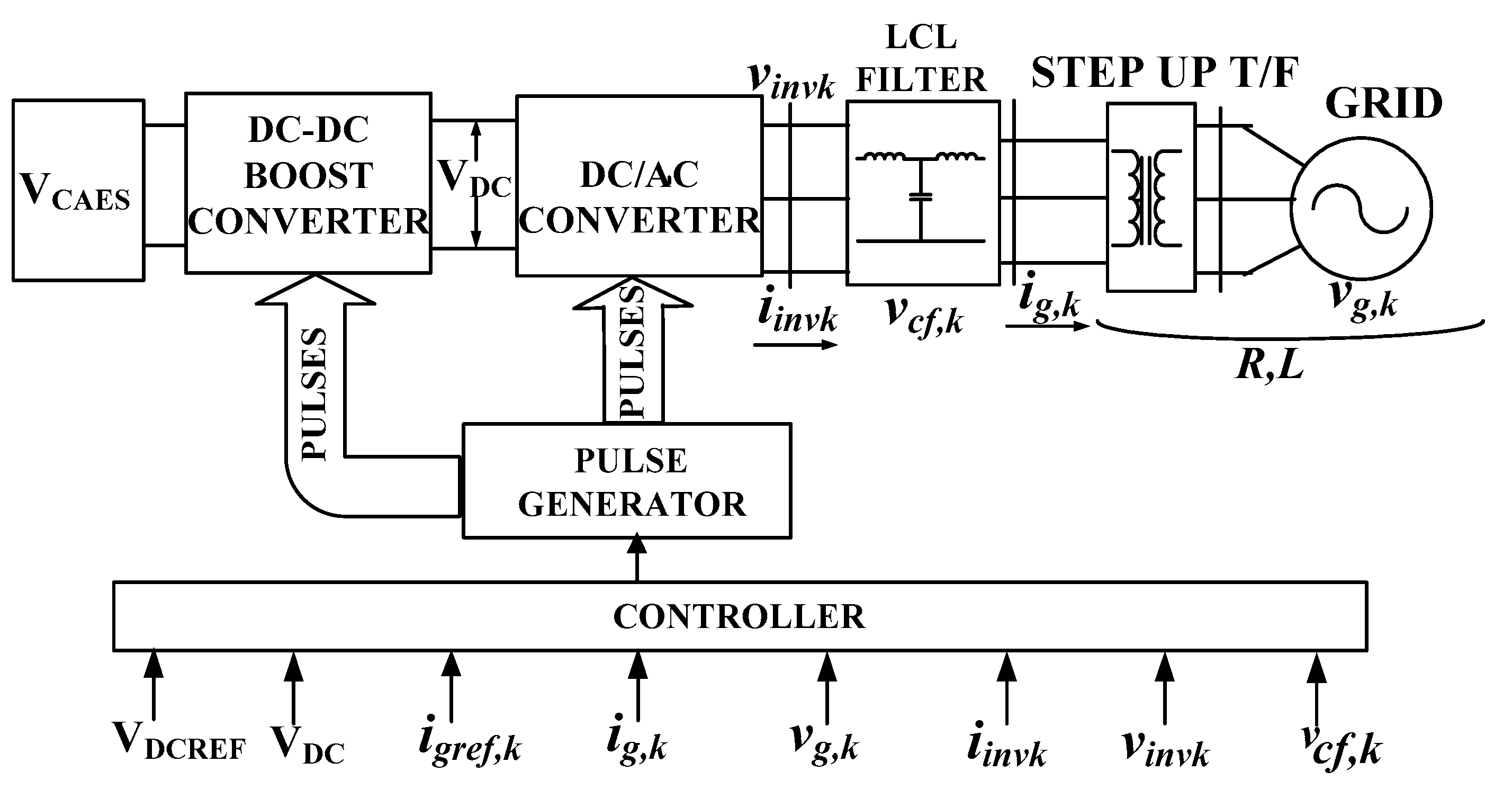
2. System Configuration

The layout of the total system under study has been shown in Figure 1. It comprises of a CAES, a DC-DC boost converter, a voltage source inverter, a filter and a step-up transformer (110 V/230 V). The output of the CAES is given to the boost converter to step up to 450 V and this boosted voltage is converted to three phase AC and connected to the grid.

During a power demand by the grid the CAES delivers the required amount of active power to the grid. The grid voltage (v_g,k), grid current (i_g,k), inverter output current (i_invk), filter capacitor voltage (v_cf,k) at the output of the inverter (where k = phase A, B, C) and DC link voltage (V_DC) are measured using voltage and current sensors. The feedback signals i_g,k and V_DC are compared to their specific references marked with the corresponding subscript “ref” to produce the error signals, which eventually are fed to the controller to produce the control signals to the system. The classical controller performance for the boost converter worsens in presence of unknown fluctuation in input supply and load due to the non-minimum phase characteristic of the boost converter.

It is important to design a power flow controller that will provide the required amount of power to the grid from the CAES. A sliding mode control based power flow controller for the VSI is developed for this purpose. For a specific power demand, the controller controls the gate pulses of the VSI to deliver the required power to the grid with maintained grid voltages.

3. Compressed Air Energy Storage Details

The micro-CAES system employed is designed around the use of an air motor. Air motors, or expanders, generate work from the expansion of compressed air. Coupling air motors with electrical generators therefore creates systems capable of converting potential energy in the form of high-pressure air into electrical power. A number of types of air motor are available, with the scroll-type air motor being chosen as the sub component owing to the robust, reliable and smooth operation [11,12]. Scroll motors are comprised of two identical interlocking scroll blades, with one fixed and the other mounted on a shaft at an offset, such that the moving scroll can rotate eccentrically around a fixed orbit. Sealed chambers are created by the meshing of the two scroll blades and depending on the stage of the orbit of the moving scroll, the chamber volumes vary. When driven with compressed air, the expansion causes work to rotate the scroll shaft.

4. Design of the System Controller

The practical circuit for the proposed work is shown in Figure 2. In this work two robust controllers have been designed: an MRAC controller for the boost converter to maintain the DC link voltage and one SMC controller to control the power flow from energy storage to grid through the VSI. The design of both controllers is described in the following subsections.

4.1. Control of DC Link Voltage

To design the MRAC controller for the boost converter to maintain the DC link voltage, the reference plant model for the converter is to be chosen first. According to the circuit diagram for the boost converter given in Figure 2, the linearized state space model around an arbitrary operating point is described as:

$$\begin{array}{c}\dot{x}=\left[\begin{array}{cc}-\frac{R}{L}& -\frac{1-D}{L}\\ \frac{1-D}{C}& -\frac{1}{R_{Load}C}\end{array}\right]x+\left[\begin{array}{c}\frac{V_C}{L}\\ -\frac{I}{C}\end{array}\right]u\\ y=\left[\begin{array}{cc}0& 1\end{array}\right]x\end{array}\}$$

(1)

where, the system states are $x={\left[\Delta \begin{array}{cc}{i}_L& \Delta v_C\end{array}\right]}^T$ and the input is $u=\left[\Delta d\right]$. I, Vc and D are the steady state values of the inductor current i_L, output voltage v_C and duty cycle d of the transistor switch T_b around the operating point and Δ corresponds to the deviation of these parameters from steady state. In the state equation R_Load is the resistance as seen by boost converter and is given by $R_{Load}=V_C^2/P_{Demand}$ with P_Demand is the required power at the output. So, from the state matrix it is clear that the zero of the boost converter system is given as:

$$z=\frac{\frac{V_C\left(1-D\right)}{I}-R}{L}$$

(2)

which is located at the right half of the s-plane and hence the system becomes non-minimum phase and non-ASPR. In order to apply the MRAC control technique the system first needs to be converted into ASPR system by adding suitable PFC to the system. The transfer function for the model in Equation (1) is of the form:

$$G\left(s\right)=\frac{Y\left(s\right)}{U\left(s\right)}=\frac{-k_{1}s+k_2}{s^2+k_{3}s+k_4}$$

(3)

where, k_i (i = 1,2,3,4) is a positive constant.

For the system in Equation (1) with L = 8.2 mH, R = 82 Ohm, C = 1120 uF, R_Load = 100 Ohm, V_c = 450 V, I = 10.12 A and D = 0.55 the root locus of the transfer function in Figure 3a shows the non-ASPR character of the system. Since, the direct MRAC technique cannot be applied to the system with non-minimum phase a PFC is designed to make it minimum phase. However, in order to keep the system dynamics intact, it must be ensured that the augmented plant output should be almost same as the actual plant output with this modification.

To design the PFC, it must be ensured that the plant is stabilizable using any controller. So, a PI controller is designed by root locus method to shift poles to the left side of the s-plane as:

$$C\left(s\right)=\frac{0.0001s+0.03}{s}$$

(4)

Now, to make the system minimum phase and of relative degree one, a PFC is designed as inverse of a PD compensator D(s) that stabilizes the series combination of C(s)G(s). The PFC is thus designed using the root locus method as:

$$PFC=D{\left(s\right)}^{-1}=\frac{0.001}{0.001s+1}$$

(5)

Figure 3b shows the root locus of the augmented system $G^{\prime }\left(s\right)=C\left(s\right)G\left(s\right)+PFC$ which is now minimum phase and of relative degree one and hence the MRAC technique can be applied to this augmented system.

The control block diagram for the MRAC based DC link voltage control is shown in Figure 4. The reference model for the controller is chosen as:

$$G_{REF}\left(s\right)=\frac{Y_m\left(s\right)}{R\left(s\right)}=\frac{b_m}{s+a_m}$$

(6)

where, a_m and b_m are positive constants.

The objective of the controller is to minimize a convex function $J\left(a\right)=0.5{e_m}^2$, where a is the adaptation parameters (a_r and a_x), e_m is the error between the desired output y_m and augmented plant output x_m and is given by:

$$e_m=x_m-y_m$$

(7)

If the error is increased due to system conditions, then the MRAC modifies the control parameters a_r and a_x so as to minimize the error.

The adjustment mechanism of conventional MRAC to change the control parameter in the direction of negative gradient of J(a) is given in [25] as:

$$\begin{array}{c}\frac{d{a}_r}{dt}=-{\gamma }^{\prime }\frac{\partial J}{\partial a_r}=-{\gamma }^{\prime }{e}_m\frac{\partial e_m}{\partial a_r}\\ \frac{d{a}_x}{dt}=-{\gamma }^{\prime }\frac{\partial J}{\partial a_x}=-{\gamma }^{\prime }{e}_m\frac{\partial e_m}{\partial a_x}\end{array}\}$$

(8)

where, γ′ is the adaptation gain.

The control law is taken as:

$$u\left(t\right)=a_r\left(t\right)r\left(t\right)-a_x\left(t\right)x_m\left(t\right)$$

(9)

From (3) and (9) it can be deduced:

$$x_m=\frac{G^{\prime }\left(s\right)a_{r}r}{1+G^{\prime }\left(s\right)a_x}$$

(10)

Substituting (10) and (6) in (7) it is found that,

$$e_m=\frac{G^{\prime }\left(s\right)a_{r}r}{1+G^{\prime }\left(s\right)a_x}-G_{REF}\left(s\right)r$$

(11)

Taking partial derivative of e_m w.r.t. adaptation parameters a_r and a_x it can be written,

$$\begin{array}{c}\frac{\partial e_m}{\partial a_r}=\frac{G^{\prime }\left(s\right)r}{1+G^{\prime }\left(s\right)a_x}\\ \frac{\partial e_m}{\partial a_x}=-\frac{G^{\prime }\left(s\right)x_m}{1+G^{\prime }\left(s\right)a_x}\end{array}\}$$

(12)

For accurate error tracking it can be assumed that,

$$1+G^{\prime }\left(s\right)a_x\approx s+a_m$$

(13)

So, from (8) and (12) it can be written,

$$\begin{array}{c}\frac{d{a}_r}{dt}=-\gamma e_m{G}_{REF}r\\ \frac{d{a}_x}{dt}=\gamma e_m{G}_{REF}{x}_m\end{array}\}$$

(14)

with, b_m absorbed in γ and normalized with static gain of one.

Combining (9) and (14) the control signal to the plant is generated. When the tracking error e_m increases these adaptation parameters get modified to change the control signal to the plant and effectively reduce the error.

Alternatively, to provide similar control quality, irrespective of the operating point, an LQR controller with integral action or a PI controller might be used with the parameters updated in real time. It is achieved via extensive experimental look-up tables, making the control design cumbersome and depending on the accuracy of the parameters measurement, or via parameters’ adaptation algorithms which still do not guarantee that the dynamical behavior is the same for all operating points.

4.2. Control of Grid Side VSI

The purpose of SMC based controller for the VSI is to control the power flow through the VSI to the grid when there is a requirement of power from the CAES. This can be achieved by using a PI controller also but, the major drawbacks are: there must be two control loops for voltage and current and the power decoupling ability between the active and reactive power is very poor in presence of disturbances in grid voltage and frequency. So, the attenuation of the controllers for one operating point does not provide required quality in the whole control range and also it is very sensitive to the accuracy of the parameters. As an alternative a simplified decoupling method has been employed to transform the system into two reduced order decoupled system and then an SMC has been designed with P_ref and Q_ref as the active and reactive power references respectively, for controlling the grid currents. The d-q reference frame rotates synchronously with the grid voltage vector and initially at t = 0 the q-axis was aligned with phase A axis vector.

The block diagram of the SMC controller is shown in Figure 5. In the system shown in Figure 2, at the point of coupling to the grid, it can be modelled as:

$$\begin{array}{c}\frac{L_f}{2}\left[\begin{array}{c}\dot{i_{dinv}}\\ \dot{i_{qinv}}\end{array}\right]=-\frac{R_f}{2}\left[\begin{array}{c}{i}_{dinv}\\ i_{qinv}\end{array}\right]+\left[\begin{array}{c}{v}_{dinv}\\ v_{qinv}\end{array}\right]-\left[\begin{array}{c}{v}_{cfd}\\ v_{cfq}\end{array}\right]-\frac{L_f}{2}\omega \left[\begin{array}{c}-i_{qinv}\\ i_{dinv}\end{array}\right]\\ \frac{L_f}{2}\left[\begin{array}{c}\dot{i_{dg}}\\ \dot{i_{qg}}\end{array}\right]=-\frac{R_f}{2}\left[\begin{array}{c}{i}_{dg}\\ i_{qg}\end{array}\right]+\left[\begin{array}{c}{v}_{cfd}\\ v_{cfq}\end{array}\right]-\left[\begin{array}{c}{v}_{dg}\\ v_{qg}\end{array}\right]-\frac{L_f}{2}\omega \left[\begin{array}{c}-i_{qg}\\ i_{dg}\end{array}\right]\\ C_f\left[\begin{array}{c}\dot{v_{cfd}}\\ \dot{v_{cfq}}\end{array}\right]=\left[\begin{array}{c}{i}_{dinv}\\ i_{qinv}\end{array}\right]-\left[\begin{array}{c}{i}_{dg}\\ i_{qg}\end{array}\right]-C_f\omega \left[\begin{array}{c}-v_{cfq}\\ v_{cfd}\end{array}\right]\end{array}\}$$

(15)

where, subscript with ‘inv’, ‘g’ and ‘cf’ corresponds to inverter output, grid and filter capacitor respectively, while, ‘d’ and ‘q’ stand for d-axis and q-axis fundamental components of the corresponding parameters respectively. This can be rearranged as a standard state space system as:

$$\dot{x}=f\left(x\right)+g\left(x\right)u$$

(16)

where,

$$f\left(x\right)=\left[\begin{array}{c}-\raisebox{1ex}{$R_f$}\!\left/ \!\raisebox{-1ex}{$L_f$}\right.i_{dg}+\raisebox{1ex}{$2$}\!\left/ \!\raisebox{-1ex}{$L_f$}\right.v_{cfd}-\raisebox{1ex}{$2$}\!\left/ \!\raisebox{-1ex}{$L_f$}\right.v_{dg}+\omega i_{qg}\\ -\raisebox{1ex}{$R_f$}\!\left/ \!\raisebox{-1ex}{$L_f$}\right.i_{dinv}-\raisebox{1ex}{$2$}\!\left/ \!\raisebox{-1ex}{$L_f$}\right.v_{cfd}+\omega i_{qinv}\\ \raisebox{1ex}{$1$}\!\left/ \!\raisebox{-1ex}{$C_f$}\right.i_{dinv}-\raisebox{1ex}{$1$}\!\left/ \!\raisebox{-1ex}{$C_f$}\right.i_{dg}+\omega v_{cfq}\\ -\raisebox{1ex}{$R_f$}\!\left/ \!\raisebox{-1ex}{$L_f$}\right.i_{qg}+\raisebox{1ex}{$2$}\!\left/ \!\raisebox{-1ex}{$L_f$}\right.v_{cfq}-\raisebox{1ex}{$2$}\!\left/ \!\raisebox{-1ex}{$L_f$}\right.v_{qg}-\omega i_{dg}\\ -\raisebox{1ex}{$R_f$}\!\left/ \!\raisebox{-1ex}{$L_f$}\right.i_{qinv}-\raisebox{1ex}{$2$}\!\left/ \!\raisebox{-1ex}{$L_f$}\right.v_{cfq}-\omega i_{dinv}\\ \raisebox{1ex}{$1$}\!\left/ \!\raisebox{-1ex}{$C_f$}\right.i_{qinv}-\raisebox{1ex}{$1$}\!\left/ \!\raisebox{-1ex}{$C_f$}\right.i_{qg}-\omega v_{cfd}\end{array}\right]\mathrm{and}g\left(x\right)=\left[\begin{array}{cc}0& 0\\ \raisebox{1ex}{$2$}\!\left/ \!\raisebox{-1ex}{$L_f$}\right.& 0\\ 0& 0\\ 0& 0\\ 0& \raisebox{1ex}{$2$}\!\left/ \!\raisebox{-1ex}{$L_f$}\right.\\ 0& 0\end{array}\right]$$

with state vector as $x={\left[\begin{array}{cccccc}{x}_1& x_2& x_3& x_4& x_5& x_6\end{array}\right]}^T={\left[i_{dg}{i}_{dinv}\begin{array}{cc}{v}_{cfd}& i_{qg}\end{array}{i}_{qinv}{v}_{cfq}\right]}^T$, input as $u={\left[\begin{array}{cc}{v}_{dinv}& v_{qinv}\end{array}\right]}^T$ and output as $y={\left[\begin{array}{cc}{i}_{dg}& i_{qg}\end{array}\right]}^T$. Now defining a new set of variables as $z_1=x_1,z_2=\dot{z_1}=\dot{x_1},z_3=\dot{z_2}=\ddot{x_1},\dot{z_3}=\stackrel{\dots }{x_1},z_4=x_4,z_5=\dot{z_4}=\dot{x_4},z_6=\dot{z_5}=\ddot{x_4},\dot{z_6}=\stackrel{\dots }{x_4}$ and assuming v_dg and v_qg as constants, system (16) can be represented as:

$$\left[\begin{array}{c}\dot{z_1}\\ \dot{z_2}\\ \dot{z_3}\\ \dot{z_4}\\ \dot{z_5}\\ \dot{z_6}\end{array}\right]=\left[\begin{array}{cccccc}0& 1& 0& 0& 0& 0\\ 0& 0& 1& 0& 0& 0\\ a_1& 0& 0& 0& 0& 0\\ 0& 0& 0& 0& 1& 0\\ 0& 0& 0& 0& 0& 1\\ 0& 0& 0& a_1& 0& 0\end{array}\right]\left[\begin{array}{c}{z}_1\\ z_2\\ z_3\\ z_4\\ z_5\\ z_6\end{array}\right]+\left[\begin{array}{c}0\\ 0\\ A_1\left(x,v_{dg}, v_{qg}\right)\\ 0\\ 0\\ A_2\left(x,v_{dg}, v_{qg}\right)\end{array}\right]+\left[\begin{array}{cc}0& 0\\ 0& 0\\ \frac{4}{L_f^2{C}_f}& 0\\ 0& 0\\ 0& 0\\ 0& \frac{4}{L_f^2{C}_f}\end{array}\right]\left[\alpha \left(x\right)+\lambda \right]$$

(17)

where,

$$\begin{gathered} a_1=-\frac{R_f^3}{L_f^3}+\frac{4R_f}{L_f^2{C}_f}+\frac{3{\omega }^2{R}_f}{L_f} \\ {A}_1\left(x\right)=-\frac{4R_f}{L_f^2{C}_f}{i}_{dinv}+\left(\frac{2R_f^2}{L_f^3}-\frac{8}{L_f^2{C}_f}-\frac{6{\omega }^2}{L_f}\right)v_{cfd}+\left(\frac{3\omega R_f^2}{L_f^2}-\frac{6\omega }{L_f{C}_f}-{\omega }^3\right)i_{qg}+\frac{6\omega }{L_f{C}_f}{i}_{qinv} \\ -\frac{6\omega R_f}{L_f^2}{v}_{cfq}-\left(\frac{2R_f^2}{L_f^3}-\frac{4}{L_f^2{C}_f}-\frac{2{\omega }^2}{L_f}\right)v_{dg}+\frac{4\omega R_f}{L_f^2}{v}_{qg} \\ {A}_2\left(x\right)=-\frac{4R_f}{L_f^2{C}_f}{i}_{qinv}+\left(\frac{2R_f^2}{L_f^3}-\frac{8}{L_f^2{C}_f}-\frac{6{\omega }^2}{L_f}\right)v_{cfq}-\left(\frac{3\omega R_f^2}{L_f^2}-\frac{6\omega }{L_f{C}_f}-{\omega }^3\right)i_{dg}-\frac{6\omega }{L_f{C}_f}{i}_{dinv} \\ +\frac{6\omega R_f}{L_f^2}{v}_{cfd}-\left(\frac{2R_f^2}{L_f^3}-\frac{4}{L_f^2{C}_f}-\frac{2{\omega }^2}{L_f}\right)v_{qg}-\frac{4\omega R_f}{L_f^2}{v}_{dg} \\ u={\left[\begin{array}{cc}{v}_{dinv}& v_{qinv}\end{array}\right]}^T=\alpha \left(x\right)+\lambda \end{gathered}$$

Considering, $\left[\begin{array}{c}{\alpha }_d\left(x\right)\\ {\alpha }_q\left(x\right)\end{array}\right]=-\frac{L_f^2{C}_f}{4}\left[\begin{array}{c}{A}_1\left(x,v_{dg},v_{qg}\right)\\ A_2\left(x,v_{dg},v_{qg}\right)\end{array}\right]$ the original 6th order system expressed by (17) can be decoupled into two independent, identical 3rd order system as:

$$\begin{array}{c}\left[\begin{array}{c}\dot{z_1}\\ \dot{z_2}\\ \dot{z_3}\end{array}\right]=\left[\begin{array}{ccc}0& 1& 0\\ 0& 0& 1\\ a_1& 0& 0\end{array}\right]\left[\begin{array}{c}{z}_1\\ z_2\\ z_3\end{array}\right]+\left[\begin{array}{c}0\\ 0\\ \frac{4}{L_f^2{C}_f}\end{array}\right]{\lambda }_d\\ \left[\begin{array}{c}\dot{z_4}\\ \dot{z_5}\\ \dot{z_6}\end{array}\right]=\left[\begin{array}{ccc}0& 1& 0\\ 0& 0& 1\\ a_1& 0& 0\end{array}\right]\left[\begin{array}{c}{z}_4\\ z_5\\ z_6\end{array}\right]+\left[\begin{array}{c}0\\ 0\\ \frac{4}{L_f^2{C}_f}\end{array}\right]{\lambda }_q\end{array}$$

(18)

Once the system is decoupled the simplified system for control can be expressed as:

$$\left[\begin{array}{c}\stackrel{\dots }{y_1}\\ \stackrel{\dots }{y_2}\end{array}\right]=\left[\begin{array}{c}\stackrel{\dots }{i_{dg}}\\ \stackrel{\dots }{i_{qg}}\end{array}\right]=a_1\left[\begin{array}{c}{i}_{dg}\\ i_{qg}\end{array}\right]+E\left[\begin{array}{c}{\lambda }_d\\ {\lambda }_q\end{array}\right]$$

(19)

where, $E=\left[\begin{array}{cc}\frac{4}{L_f^2{C}_f}& 0\\ 0& \frac{4}{L_f^2{C}_f}\end{array}\right]=\left[\begin{array}{cc}{E}_1& 0\\ 0& E_1\end{array}\right]$.

So, the SMC need to be designed to track only one of the outputs and the other one will be identical to it.

As the relative degree of system in (19) is 3 the sliding surface for the tracking algorithm is chosen as:

$$\sigma =\ddot{e_r}+m_2\dot{e_r}+m_1{e}_r+m_0{\displaystyle \int }{e}_{r}d\tau$$

(20)

with m_i (I = 0, 1, 2) are positive constants and e_r is error in the output vector, which is defined as:

$$\begin{array}{c}{e}_r{}_{idg}=i_{dg}-i_{dgref}\\ e_r{}_{iqg}=i_{qg}-i_{qgref}\end{array}\}$$

(21)

The reference values are computed from the following equations.

$$\begin{array}{c}{i}_{dgref}=\frac{2\left(v_{qg}{Q}_{ref}+v_{dg}{P}_{ref}\right)}{3\left(v_{dg}^2+v_{qg}^2\right)}\\ i_{qgref}=\frac{2\left(v_{qg}{P}_{ref}-v_{dg}{Q}_{ref}\right)}{3\left(v_{dg}^2+v_{qg}^2\right)}\end{array}\}$$

(22)

The SMC λ_d (or λ_q) need to be designed such that in finite time σ = 0 which yields the sliding variable dynamic characteristic as:

$$\dot{\sigma }=\stackrel{\dots }{e_r}+\left(m_2\ddot{e_r}+m_1\dot{e_r}+m_0{e}_r\right)$$

(23)

Assuming the reference currents remain constant during the control response it is found that,

$$\begin{array}{l}\dot{\sigma }=\stackrel{\dots }{i_{dg}}+\left(m_2\ddot{e_r}+m_1\dot{e_r}+m_0{e}_r\right)\\ =a_1{i}_{dg}+E_1{\lambda }_d+m_2\ddot{i_{dg}}+m_1\dot{i_{dg}}+m_0{i}_{dg}\\ =\left(a_1+m_0\right)i_{dg}+m_1\dot{i_{dg}}+m_2\ddot{i_{dg}}+E_1{\lambda }_d\\ =F\left(i_{dg},\dot{i_{dg}},\ddot{i_{dg}}\right)+E_1{\lambda }_d\end{array}$$

(24)

where, $F\left(i_{dg},\dot{i_{dg}},\ddot{i_{dg}}\right)$ is assumed bounded, i.e., $\left|F\left(i_{dg},\dot{i_{dg}},\ddot{i_{dg}}\right)\right|\le N$.

To satisfy Lyapunov’s global finite-time stability criterion it is required.

$$\dot{V}=\sigma \dot{\sigma }\le -\frac{\alpha }{\surd 2}\left|\sigma \right|$$

(25)

with $\alpha =constant>0$. Selecting ${\lambda }_d=-\rho sign\left(\sigma \right)$ where ρ is a positive constant and using (24) it can be shown:

$$\begin{array}{l}\dot{\sigma }=\sigma \left(F\left(i_{dg},\dot{i_{dg}},\ddot{i_{dg}}\right)-E_1\rho sign\left(\sigma \right)\right)\\ =\sigma F\left(i_{dg},\dot{i_{dg}},\ddot{i_{dg}}\right)-E_1\rho \left|\sigma \right|\\ =\left(sign\left(\sigma \right)F\left(i_{dg},\dot{i_{dg}},\ddot{i_{dg}}\right)-E_1\rho \right)\left|\sigma \right|\end{array}$$

(26)

Comparing (25) and (26) the condition for stability is found as:

$$\rho \ge \frac{\alpha }{\sqrt{2}{E}_1}+\frac{1}{E_1}sign\left(\sigma \right)F\left(i_{dg},\dot{i_{dg}},\ddot{i_{dg}}\right)$$

(27)

As the maximum positive value for $\frac{1}{E_1}sign\left(\sigma \right)F\left(i_{dg},\dot{i_{dg}},\ddot{i_{dg}}\right)$ is $\frac{N}{E_1}$ the value for ρ should be,

$$\rho \ge \frac{\alpha }{\sqrt{2}{E}_1}+\frac{N}{E_1}$$

(28)

This value for ρ is same for both the SMC λ_d and λ_q.

For any imperfection in the decoupling, (19) is modified as:

$$\left[\begin{array}{c}\stackrel{\dots }{y_1}\\ \stackrel{\dots }{y_2}\end{array}\right]=\left[\begin{array}{c}\stackrel{\dots }{i_{dg}}\\ \stackrel{\dots }{i_{qg}}\end{array}\right]=a_1\left[\begin{array}{c}{i}_{dg}\\ i_{qg}\end{array}\right]+\left[\begin{array}{c}\Delta A_1\left(x,v_{dg},v_{qg}\right)\\ \Delta A_2\left(x,v_{dg},v_{qg}\right)\end{array}\right]+E\left[\begin{array}{c}{\lambda }_d\\ {\lambda }_q\end{array}\right]$$

(29)

In that case, deriving in the same manner the condition for stability is found as:

$$\begin{array}{c}{\rho }_d\ge \frac{\alpha }{\sqrt{2}{E}_1}+\frac{1}{E_1}\left(N+\left|\Delta A_1\left(x,v_{dg},v_{qg}\right)\right|\right)\\ {\rho }_q\ge \frac{\alpha }{\sqrt{2}{E}_1}+\frac{1}{E_1}\left(N+\left|\Delta A_2\left(x,v_{dg},v_{qg}\right)\right|\right)\end{array}\}$$

(30)

From (30) it can be observed that for bounded disturbance ΔA the SMC parameter ρ is also bounded and the system will be stabilized.

With use of ‘sign()’ function in the analysis it may also create chattering problem which can be reduced by choosing similar function ‘tanh()’ and proper value of ρ.

5. Simulation Results

The entire system control is simulated in MATLAB/SIMULINK environment using the ideal switches and elements of Simscape toolbox to check the feasibility of the system. The MRAC and SMC controller are designed as discussed in Section 4. The parameters for the design are presented in

Table 1. Simulation parameter.

System Parameter	Value
Lf/2	1.64 mH, 7.2 A
Cf	10 μF, 305 V
Cin	470 μF, 400 V
L	8.2 mH, 7.2 A
R	82 Ω, 150 W
Transformer turns ratio	110:230
DC-link Voltage	450 V
Grid Voltage	230 V
Switching frequency	5 kHz
Adaptation gain γ	0.8
Sliding mode gain ρ	9

.

5.1. DC Side Controller

The performance of the DC side controller has been investigated for different input voltage and load conditions. Figure 6 shows the DC-link voltage for variation in the input voltage from the CAES keeping the load constant at R_Load = 100 Ohm. The boost converter starts operating from t = 1 s and then for variation in the CAES input voltage, the output DC-link voltage is found to be maintained at 450 V.

The corresponding inductor and output currents of the boost converter are shown in Figure 7. It is seen that at the starting of the boost converter the current peak is very high but at the later stage for variation in the voltage the current peaks are within limit. This starting current can be limited by using a charging resistor in series with the boost converter and once the current is within limit it is short-circuited.

The transient response of the boost converter with a standard PI controller and MRAC controller for two loading conditions is shown in Figure 8. The gains of the PI controller are chosen to be K_p = 0.1 and K_i = 1 for minimum settling time possible for the system under test with acceptable ripple of 2% and without overshoot condition.

The response shows that with the MRAC controller the output voltage settles to reference voltage in 0.121 s whereas with the PI controller, it settles in 0.528 s for a fall of 50 V in the input voltage at t = 1.71 s and R_Load = 10 Ohm. Similarly, for R_Load = 100 Ohm the settling time for the output voltage remains almost same for the same dip in the input voltage but, comparatively larger oscillations are added in case of PI controller. This proves the faster operation and better damping property of the MRAC. This operation can be made even faster with choice of higher value of adaptation parameter γ. However, the overshoot in the output voltage also rises with it. So, an optimum value of adaptation parameter γ as given in Table 1 is chosen for this simulation.

5.2. Grid Side Controller

The performance of the SMC controller to control the power flow through the VSI to the grid from the CAES has also been analyzed in simulation for different power demand scenario.

Figure 9a shows the inverter output voltage for different power flow conditions. The switch S₃ between inverter side and grid has been closed at t = 0.1 s. It can be seen from Figure 9b that inverter phase-A reference voltage and the grid voltage of phase-A are synchronized with each other for successful integration with the grid. The command for power requirement by the grid has been given at t = 0.15 s and the grid current increases accordingly to meet the power demand of 600 W, keeping the voltage unchanged. The corresponding inverter currents in d-q reference frame have been shown in Figure 9c. At t = 0.6 s the power demand rises from 600 W to 1500 W and again at t = 1.2 s it reduces to 600 W. From Figure 9d it is clear that the inverter system is able to comply the power demand requirement by the grid successfully.

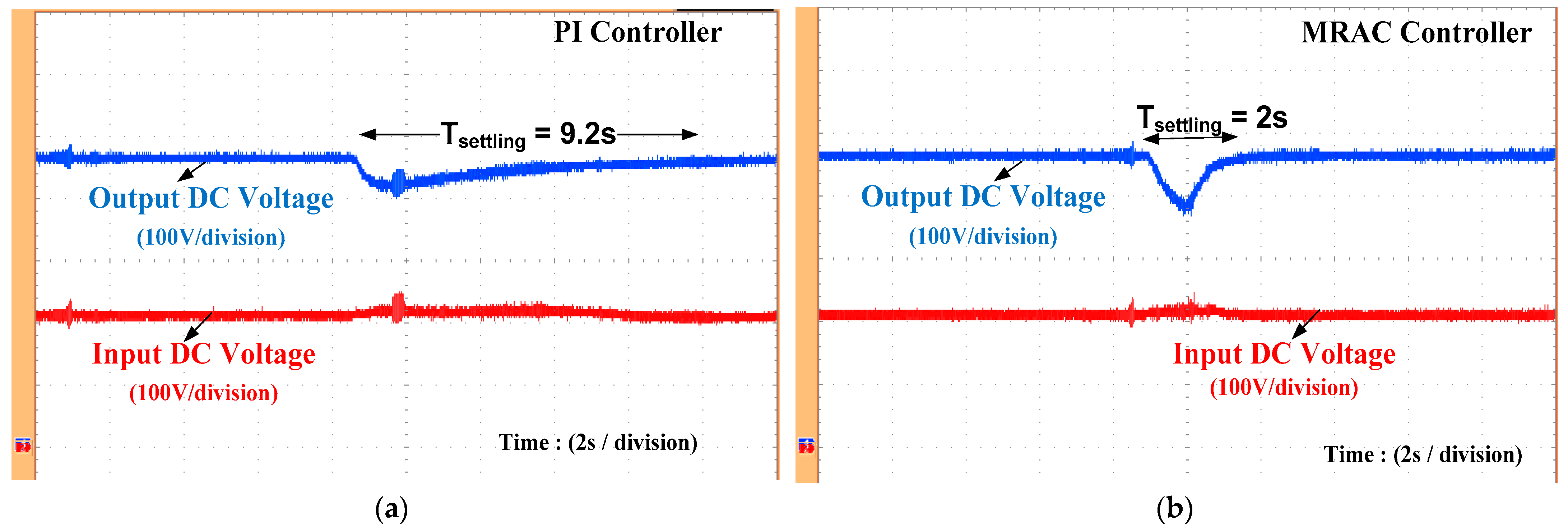
6. Experimental Results

The proposed two stage grid tied micro-CAES system using a boost converter and a VSI has been verified in the hardware setup in OPAL-RT platform. The hardware setup developed for the system under study is shown in Figure 10.

The scroll-type air motor employed in the experimental system is an Air Squared Mfg. 1 kW device. The device is fed from a 340 L air tank charged with air at up to 20 bar from a grid fed compressor. The air flow into the scroll is controlled by a pressure regulating valve. The scroll-air motor is coupled with a Voltmaster AB30L 2.4 kW induction generator, whose output voltage is then rectified to DC and used as input for the other system components. The inputs and outputs to the micro-CAES system at different air pressures can be observed in Figure 11. The input pressure to the expander is incrementally increased in steps of 1 bar. The generator cuts in when the pressure increases to over 2.5 bar and an output voltage from the generator is achieved. It can be observed that the output voltage from the CAES system generator is proportional to the input pressure to the air motor.

The controllers have been designed in MATLAB and interfaced to the system via OPAL-RT. The feedback signals are acquired from the actual system using voltage and current sensors and then fed to the controllers through ADC converters.

To prove the efficacy of the MRAC the grid tied CAES system has been tested in real time hardware setup and the DC-link voltage is compared with PI control. Figure 12a shows that for a rise in power demand from zero to 934 W the DC-link voltage falls and then the controller drives it back to its reference voltage after 9.2 s for the PI controller, whereas the proposed MRAC controller takes only 2 s to settle the voltage to its reference level as can be seen from Figure 12b. The deviation in settling time of the simulation result and that of experimental result is due to the use of a rate limiter in the experimental setup with slew rate of 200 for smooth operation. However, it can be noted that the ratio of settling time for MRAC and PI control technique remains approximately same in both simulation and experimental result.

The effect of variation in CAES voltage on the DC-link voltage and inverter current is shown in Figure 13a,b. It is seen that the variation in the input voltage from 200 V to 150 V and vice versa has negligible effect on the output current of the system. So, the power flow remains unaltered at 710 W for input side disturbances which proves the effectiveness of the MRAC controller.

The inverter output should be in phase with the grid and match the frequency of the grid voltage. Figure 14a shows that the inverter voltage and grid current waveforms have the same frequency with the unity power factor, which satisfies the condition for the grid integration of the inverter. The waveform for the three phase inverter current for the 934 W power delivery condition is shown in Figure 14b.

The power flow reference is fed to the system in terms of the reference current I_dgref and I_qgref. Figure 15a,b shows one phase inverter current with the change in the reference power. In Figure 15a it is shown that a step change of power delivery from 710 W to 934 W has been made by changing the reference current I_dgref from 3 A to 4 A based on (22). As a result, the SMC controller generates the actuating signal such that the inverter current (rms) changes from 2.15 A to 2.83 A. Similarly, for a fall in power demand from 934 W to 710 W, the inverter current (rms) again changes from 2.83 A to 2.15 A as shown in Figure 15b. In both the cases I_qgref has been kept as zero. From the experimental results it is verified that any power demand by the grid can be delivered with faster response and high efficiency by the grid connected CAES based system with the designed controller.

7. Conclusions

A grid integrated compressed air energy storage system with modern non-linear control techniques has been presented in this paper. The complete system uses a two-stage conversion with a model reference adaptive controlled DC–DC boost converter and sliding mode-controlled voltage source inverter to integrate the energy storage device to the grid. The conventional control techniques require a detail knowledge of system parameters and they respond efficiently for known disturbances only. In the presented work the MRAC and SMC controllers can address any kind of disturbances arising in the system due to parametric changes and operating point shifting, making the system more robust. The total system has been simulated in the MATLAB/SIMULINK environment with different operating conditions and the results have been presented that prove the better performance of the system. Moreover, the conclusions drawn from the simulation are also tested in a real time hardware setup with the OPAL-RT platform and validated to claim the efficacy of the system.

References

1. Hansen, K.; Breyer, C.; Lund, H. Status and perspectives on 100% renewable energy systems. Energy 2019, 175, 471–480. [Google Scholar] [CrossRef]
2. Pleßmann, G.; Erdmann, M.; Hlusiak, M.; Breyer, C. Global Energy Storage Demand for a 100% Renewable Electricity Supply. Energy Procedia 2014, 46, 22–31. [Google Scholar] [CrossRef] [Green Version]
3. Bazilian, M.; Mai, T.; Baldwin, S.; Arent, D.; Miller, M.; Logan, J. Decision-making for High Renewable Electricity Futures in the United States. Energy Strat. Rev. 2014, 2, 326–328. [Google Scholar] [CrossRef]
4. Lund, P.D.; Lindgren, J.; Mikkola, J.; Salpakari, J. Review of energy system flexibility measures to enable high levels of variable renewable electricity. Renew. Sustain. Energy Rev. 2015, 45, 785–807. [Google Scholar] [CrossRef] [Green Version]
5. Brouwer, A.S.; van den Broek, M.; Seebregts, A.; Faaij, A. Impacts of large-scale Intermittent Renewable Energy Sources on electricity systems, and how these can be modeled. Renew. Sustain. Energy Rev. 2014, 33, 443–466. [Google Scholar] [CrossRef]
6. Weitemeyer, S.; Kleinhans, D.; Vogt, T.; Agert, C. Integration of Renewable Energy Sources in future power systems: The role of storage. Renew. Energy 2015, 75, 14–20. [Google Scholar] [CrossRef] [Green Version]
7. Hu, J.; Harmsen, R.; Crijns-Graus, W.; Worrell, E.; van den Broek, M. Identifying barriers to large-scale integration of variable renewable electricity into the electricity market: A literature review of market design. Renew. Sustain. Energy Rev. 2018, 81, 2181–2195. [Google Scholar] [CrossRef]
8. Mears, D.; Gotschall, H.; Kamath, H. EPRI-DOE Handbook of Energy Storage for Transmission and Distribution Applications; EPRI: Palo Alto, CA, USA; The U.S. Department of Energy: Washington, DC, USA, 2003.
9. Evans, A.; Strezov, V.; Evans, T.J. Assessment of utility energy storage options for increased renewable energy penetration. Renew. Sustain. Energy Rev. 2012, 16, 4141–4147. [Google Scholar] [CrossRef]
10. Wang, J.; Lu, K.; Ma, L.; Wang, J.; Dooner, M.; Miao, S.; Li, J.; Wang, D. Overview of Compressed Air Energy Storage and Technology Development. Energies 2017, 10, 991. [Google Scholar] [CrossRef] [Green Version]
11. Wang, J.; Yang, L.; Luo, X.; Mangan, S.; Derby, J.W. Mathematical Modeling Study of Scroll Air Motors and Energy Efficiency Analysis—Part I. IEEE/ASME Trans. Mechatron. 2011, 16, 112–121. [Google Scholar] [CrossRef]
12. Wang, J.; Luo, X.; Yang, L.; Shpanin, L.M.; Jia, N.; Mangan, S.; Derby, J.W. Mathematical Modeling Study of Scroll Air Motors and Energy Efficiency Analysis—Part II. IEEE/ASME Trans. Mechatron. 2009, 16, 122–132. [Google Scholar] [CrossRef]
13. Luo, X.; Wang, J.; Dooner, M.; Clarke, J. Overview of current development in electrical energy storage technologies and the application potential in power system operation. Appl. Energy 2015, 137, 511–536. [Google Scholar] [CrossRef] [Green Version]
14. Kim, Y.; Favrat, D. Energy and exergy analysis of a micro-compressed air energy storage and air cycle heating and cooling system. Energy 2010, 35, 213–220. [Google Scholar] [CrossRef] [Green Version]
15. Tallini, A.; Vallati, A.; Cedola, L. Applications of Micro-CAES Systems: Energy and Economic Analysis. Energy Procedia 2015, 82, 797–804. [Google Scholar] [CrossRef] [Green Version]
16. Todorovic, M.H.; Palma, L.; Enjeti, P.N. Design of a wide input range DC–DC converter with a robust power control scheme suitable for fuel cell power conversion. IEEE Trans. Ind. Electr. 2008, 55, 1247–1255. [Google Scholar] [CrossRef]
17. Sira-Ramirez, H.; Rios-Bolívar, M. Sliding mode control of DC-to-DC power converters via extended linearization. IEEE Trans. Circuits Syst. 1994, 41, 652–661. [Google Scholar] [CrossRef]
18. Hiti, S.; Borojevic, D. Robust nonlinear control for boost converter. IEEE Trans. Ind. Electr. 1995, 10, 651–658. [Google Scholar]
19. Sun, L. Helicopter Hovering Control Design based on Model Reference Adaptive Method. In Proceedings of the 2019 IEEE 3rd Information Technology, Networking, Electronic and Automation Control Conference (ITNEC), Chengdu, China, 15–17 March 2019; pp. 1621–1624. [Google Scholar]
20. Morse, W.D.; Ossman, K.A.; Ossman, A. Model following reconfigurable flight control system for the AFTI/F-16. J. Guid. Control. Dyn. 1990, 13, 969–976. [Google Scholar] [CrossRef]
21. Bar-Kana, I.; Fischl, R. A Simple Adaptive Enhancer of Voltage Stability for Generator Excitation Control. In Proceedings of the 1992 American Control Conference, Chicago, IL, USA, 24–26 June 1992; pp. 1705–1709. [Google Scholar]
22. Bar-Kana, I.; Guez, A. Simplified Techniques for Adaptive Control of Robotic. In Control and Dynamic Systems—Advances in Theory and Applications; Leondes, C., Ed.; Elsevier: Amsterdam, The Netherlands, 1991; Volume 41, pp. 147–203. [Google Scholar]
23. Chen, J.; Wang, J.; Wang, W. Model Reference Adaptive Control for a Class of Aircraft with Actuator saturation. In Proceedings of the 2018 37th Chinese Control Conference (CCC), Wuhan, China, 25–27 July 2018; pp. 2705–2710. [Google Scholar]
24. Kurniawan, E.; Widiyatmoko, B.; Bayuwati, D.; Afandi, M.I.; Suryadi; Rofianingrum, M.Y. Discrete-Time Design of Model Reference Learning Control System. In Proceedings of the 2019 24th International Conference on Methods and Models in Automation and Robotics (MMAR), Miedzyzdroje, Poland, 26–29 August 2019; pp. 337–341. [Google Scholar]
25. Mizumoto, I.; Iwai, Z. Simplified adaptive model output following control for plants with unmodelled dynamics. Int. J. Control 1996, 64, 61–80. [Google Scholar] [CrossRef]
26. Khajehoddin, S.A.; Karimi-Ghartemani, M.; Jain, P.K.; Bakhshai, A. A Control Design Approach for Three-Phase Grid-Connected Renewable Energy Resources. IEEE Trans. Sustain. Energy 2011, 2, 423–432. [Google Scholar] [CrossRef]
27. Bao, X.; Zhuo, F.; Tian, Y.; Tan, P. Simplified Feedback Linearization Control of Three-phase Photo-voltaic Inverter with an LCL Filter. IEEE Trans. Power Electron. 2012, 28, 2739–2752. [Google Scholar] [CrossRef]
28. He, N.; Xu, D.; Zhu, Y.; Zhang, J.; Shen, G.; Zhang, Y.; Ma, J.; Liu, C. Weighted Average Current Control in a Three-Phase Grid Inverter with an LCL Filter. IEEE Trans. Ind. Electron. 2012, 28, 2785–2797. [Google Scholar] [CrossRef]
29. Mishra, S.; Sekhar, P.C. Sliding mode based feedback linearizing controller for a PV system to improve the performance under grid frequency variation. In Proceedings of the 2011 International Conference on Energy, Automation and Signal, Bhubaneswar, India, 28–30 December 2011; pp. 1–7. [Google Scholar]
Figure 1. Block diagram of the system under study.
Energies 14 04097 g001
Figure 2. Block diagram of the system under study.
Energies 14 04097 g002
Figure 3. Root locus of the (a) uncompensated system; (b) compensated system.
Energies 14 04097 g003
Figure 4. Control block diagram of MRAC controller for boost converter.
Energies 14 04097 g004
Figure 5. Control block diagram of SMC controller for VSI.
Energies 14 04097 g005
Figure 6. Input CAES voltage and DC-link voltage for boost converter.
Energies 14 04097 g006
Figure 7. Input current and output current of the boost converter.
Energies 14 04097 g007
Figure 8. Output voltage of the boost converter for fall in input voltage with MRAC and PI controller.
Energies 14 04097 g008
Figure 9. (a) Three phase inverter reference voltage, grid voltage and grid current; (b) inverter reference voltage and grid voltage of phase-A, (c) Id and Iq of inverter output current; (d) active and reactive power flow to the grid.
Energies 14 04097 g009
Figure 10. Experimental setup of the grid integrated CAES system.
Energies 14 04097 g010
Figure 11. CAES output voltage with different air flow rate and air pressure.
Energies 14 04097 g011
Figure 12. (a) Input and output voltage of the boost converter for a rise in power demand with PI controller; (b) input and output voltage of the boost converter for a rise in power demand with MRAC controller.
Energies 14 04097 g012
Figure 13. (a) Inverter current (phase A) and DC-link voltage for fall in input CAES voltage; (b) inverter current (phase A) and DC-link voltage for increase in input CAES voltage.
Energies 14 04097 g013
Figure 14. (a) Grid current and inverter reference voltage with unity power factor; (b) three phase inverter current for 934 W power delivery.
Energies 14 04097 g014
Figure 15. (a) Inverter current for rise in Idgref, (b) inverter current for fall in Idgref.
Energies 14 04097 g015