Article

A Cascade Proportional Integral Derivative Control for a Plate-Heat-Exchanger-Based Solar Absorption Cooling System

by
Yeudiel Garcíadealva
1,*,
Roberto Best
1,
Víctor Hugo Gómez
1,
Alejandro Vargas
2,
Wilfrido Rivera
1 and
José Camilo Jiménez-García
1
1
Instituto de Energías Renovables (IER), Universidad Nacional Autónoma de México (UNAM), 62588 Temixco, Mexico
2
Unidad Académica Juriquilla, Instituto de Ingeniería, Universidad Nacional Autónoma de México (UNAM), 76230 Querétaro, Mexico
*
Author to whom correspondence should be addressed.
Energies 2021, 14(13), 4058; https://doi.org/10.3390/en14134058
Submission received: 14 May 2021 / Revised: 9 June 2021 / Accepted: 16 June 2021 / Published: 5 July 2021

Abstract

:
Automatic proportional integral derivative control techniques are applied in a single-stage solar absorption cooling system, showing 3.8 kW (~1 ton) cooling capacity, with a coefficient of performance of 0.6 and −4.1 °C evaporator cooling temperature. It is built with plate heat exchangers as main components, using ammonia–water as the working mixture fluid and solar collectors as the main source of hot water. Control tuning was verified with a dynamical simulation model for a solution regarding mass flow stability and temperature control in the solar absorption cooling system. The controller improved steady thermodynamic state and time response. According to experimental cooling temperatures, the system could work in ranges of refrigeration or air-conditioning end-uses, whose operation makes this control technique an attractive option to be implemented in the solar absorption cooling system.

1. Introduction

Since 1990, there has been a more than threefold increase in the demand for space cooling in buildings. Space cooling contributed with the emission of 1 Gt CO2 and around 8.5% of global electricity consumption, according to the 2019 global energy report [1]. Some reasons are: the improvement in environmental comfort, urban growth, and climatic changes that cause drastic variations in temperatures. Following the same trend over the years, cooling demand growth rates will continue in the next decade. China has positioned itself as the world leader, with 40% of the market in the purchase of cooling equipment [1]. It has been recorded that global refrigeration consumption is the cause of 15% of electricity demand peaks, and for days of intense heat, it can be responsible for more than 50% of electricity demand peaks in the residential sector [2].
Absorption cooling systems are being used worldwide to save electricity, with chillers driven by waste heat, district heat, or solar heat. The evidence that the peak cooling demand is linked with increased solar radiation presents an optimal development opportunity for solar thermal refrigeration technologies. An example of experimental absorption equipment is a system, whose components, i.e., the heat exchangers, the expansion valve, and the thermal compressor, are connected by means of pipes and valves, which provoke strong non-linearities, a high dependency unit, and a high thermal inertia. Thus, the dynamic modelling and control of such systems is not trivial [3].
Various types of absorption systems, research on working fluids, practical achievements, and the most promising developments are discussed by Ziegler [4,5,6], Labus et al. [7], Azher et al. [8], and Pongsid et al. [9]. Absorption cycles are modelled and compared with experiments by Dincer et al. [10,11] and Ng et al. [12], for different heat exchange technologies, e.g., with plate exchangers such as those proposed by Sterner and Sunden [13] and Goodarzi et al. [14].
A useful tool in the analysis of the heat and mass transfer processes, particularly during the operation set up, is the use of dynamic models [15,16,17]; Kim and Ferreira [18] achieved an analysis simulation of an ammonia–water absorption chiller. Weihua et al. [19], Viswanathan et al. [20], and Martinho et al. [21] described the dynamic model in detail regarding the heat and mass balances, whereas Iranmanesh and Mehrabian [22], Ochoa et al. [23], and Kohlenbach and Ziegler [24] describe LiBr/H2O systems, where the latter further includes performance analysis, sensitivity checks, and comparison to experimental data. Puig et al. [25] compared approaches to the characteristic equation method and concluded that the method developed by Albers et al. [26,27] is the simplest and that it provides better accuracy. An object-oriented simulation using parallel processing for foretelling the transient behavior of absorption chillers with arbitrary configuration has been explained by Matsushima et al. [28]. Other modeling methods such as state-space, graph-theory, structure-matrix, and combined forecasting have been employed for modeling air-conditioning systems by Yao et al. [29], Omar and Micallef [30], and Wen et al. [31].
An advantage of the absorption refrigeration systems over mechanical compression is the energy source; the latter require high-quality energy for their operation, but absorption refrigeration systems can use low quality thermal energy. This means that heat source temperatures do not need to be high (80–150 °C). Therefore, the waste heat from many industrial processes or, as in the actual analysis, a solar collector system would be sufficient to supply the power required in these machines, which are frequently controlled by on–off or proportional–integral control strategies. Fernández and Vázquez [32], Rêgo et al. [33], and Jeong et al. [34] propose a parametric model control action that is based on generator heat flux modulation and the level of a high temperature generator that provides the maximum system performance. Hüls et al. [35] shows applications with an intelligent control algorithm, in which absorption chillers are advantageous because of synergies within the rest of the energy supply system, such as a solar cooling system. The control of absorption commercial chillers is conventionally done by temperature control of the driving heat input. In order to understand this behavior, it is important to realize that an absorption chiller is a device that is totally governed by heat transfer processes. This gives rise to the possibility of reducing the complex response to the characteristic temperature equation model [36]. Nienborg et al. [37] contested variants of control in diverse system arrangement with a dynamic system simulation. By the optimization of key parts, they achieved electricity savings of up to 25%. Sabbagh and Gómez [38] established an optimal control strategy to run an absorption refrigeration chiller.
Some researchers have already worked with the proportional integral derivative (PID) controller [39,40,41], even using fuzzy logic [42], to tune PID parameters (Kp, Ki, and Kd) of variable speed pumps for the purpose of improving the solar fraction and the system energy consumption [43]. Lima et al. [44] proposed a technique for varying the speed of the pump and, therefore, ensured the range of flow for absorption chillers, with the pair LiBr-H2O, implementing a PID controller action system, which allowed flow control testing. Vinther et al. [45] simulated decentralized control structures in terms of PI feedback loops for absorption cycle heat pumps using the dynamic nonlinear model of a single-effect LiBr-H2O absorption system.
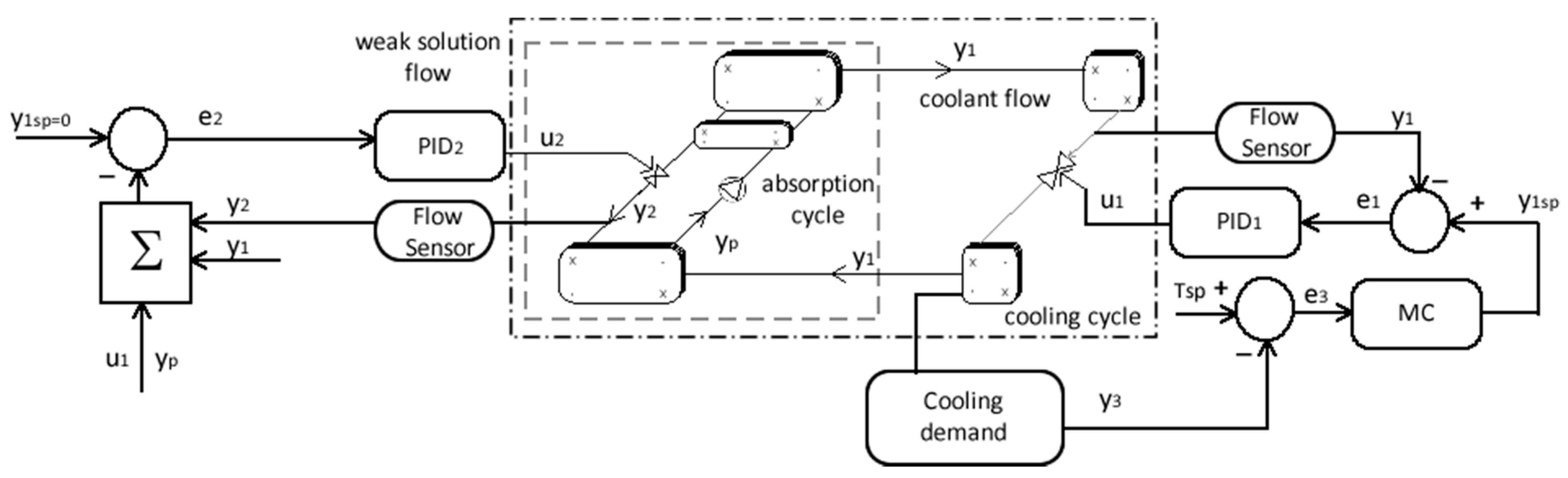
Previous work experience and promising results achieved in solar absorption systems motivate us to continue improving the systems and the models that describe them for the implementation of optimal controls. The main purpose of this work is to propose a PID controller in a plate heat exchanger solar absorption cooling system (SACS), designed and built by Jimenez-García and Rivera [46]. The system works with the ammonia–water pair (NH3–H2O), it was built using five vertical plate heat exchangers and is designed to operate with solar energy or some other cheap heat source. Suggested adjustments were made to improve efficiency; in addition, a cascade PID control is tested. The controlled variables are the outlet temperature of the cold water and the mass balance in the thermal compressor, while the solution returning to the absorber and the refrigerant volumetric flow are the manipulated variables. The test facility was located at the Refrigeration and Heat Pump Laboratory of the Renewable Energy Institute (IER), National Autonomous University of Mexico (UNAM) in Temixco, Morelos.

2. Absorption Cooling System ACS

2.1. Main System

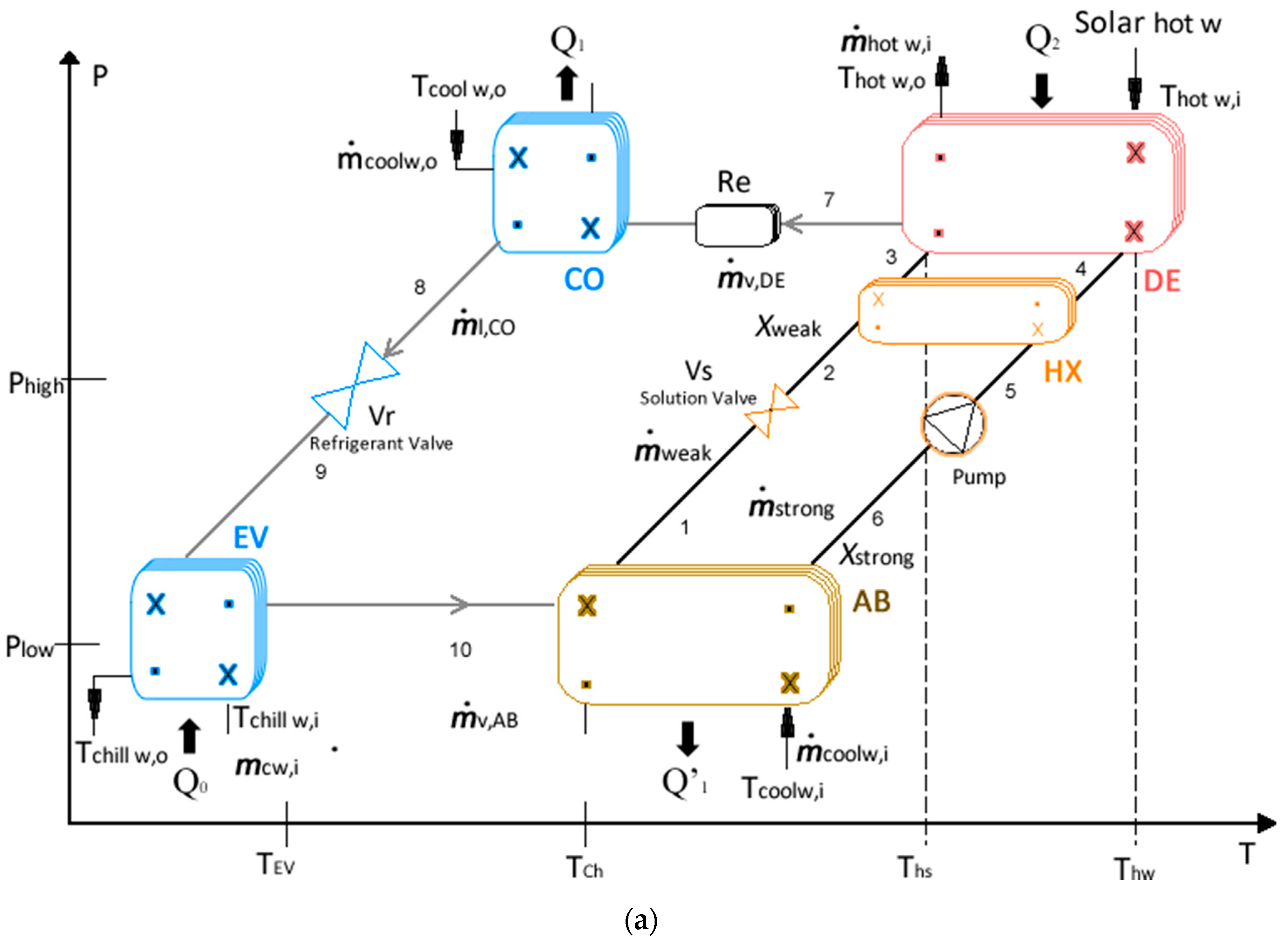
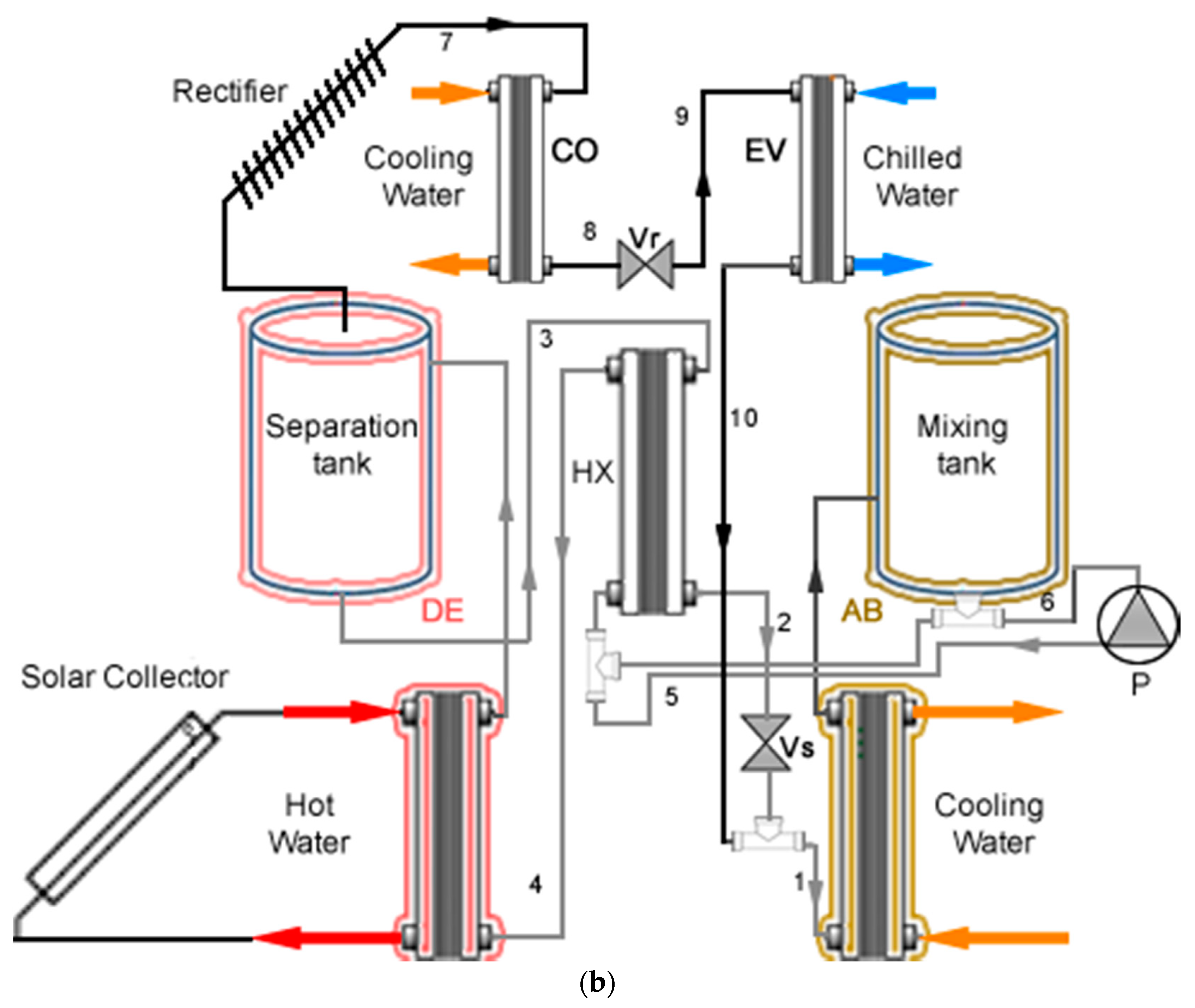
Figure 1 shows the most important components of the refrigerant (NH3) circuit: the compression heat pump, the condenser CO, the refrigerant throttling valve Vr, and the evaporator EV; heat exchangers have 20 plates each. To replace the compressor in a conventional refrigeration system, the absorber AB is used, together with a heat exchanger HX and the desorber DE (also called generator elsewhere), with 40 plates each; a solution pump P and throttling solution valve Vs are also required. In this inner circuit, a solution of the refrigerant and absorbent is recirculated. Two tanks are used, one mixing chamber in the absorber and another for vapor separation flow at DE exit. The system operation is continuous, with simultaneous refrigerant generation and absorption operations; the real experimental equipment is shown in Figure 2. Therefore, there are two circuits in the system, one for the solution (1–6) and another one for the refrigerant (7–10). External fluids are streams of water supplied to different components so that the operation of the cooling system is carried out.
In the evaporator EV, the liquid refrigerant is vaporized at low pressure by absorbing heat Q0 from the chamber to be cooled. The refrigerant vapor (10) is then absorbed by a refrigerant-depleted weak (1) solution in the absorber. The resulting strong (6) solution enriched by the absorption of refrigerant is pumped by the solution pump into DE (5), which is at the condenser pressure. The mechanical work supplied to the solution pump is relatively low, a very low percentage of the heat supplied to the desorber [5].
The pumped solution flows through HX, (4) before it enters DE, increasing its temperature as a consequence of the heat transferred by the solution returning from the desorber to the absorber. In DE, the strong solution is boiled by the driving heat Q2 at the highest temperature, whereby the refrigerant absorbed in AB is expelled from the solution (3). The refrigerant is condensed in CO (7). The condensate is then expanded in Vr (8) to the evaporator pressure (9). This closes the working medium circuit. At DE, the solution changes from high refrigerant concentration to low refrigerant concentration by the supply of heat from an external source, Q2. This weak solution flows into the solution heat exchanger HX, and then, it is expanded by the expansion valve Vs to the evaporator pressure and passes back into the absorber AB, where it can absorb refrigerant again. This closes the solution cycle.
The refrigeration cycle can be considered as a reverse thermal machine. Carnot efficiency can be defined for the refrigeration cycle as Equation (1),
( C O P ) R = T E V ( T C O T E V )  
It represents the maximum theoretical value of efficiency that can be obtained in a refrigeration cycle. In practice, the efficiencies obtained are much lower due to the irreversibilities in the system. As the analysis of the Carnot cycle gives the maximum coefficient of performance (COP)max for a mechanical vapor compression system, it is convenient to find the COP achievable in an absorption system. The heating medium of the DE supplies the heat QDE (Q2) to the system, the pump supplies the work Wp, and the cooled solution in the evaporator supplies the heat QEV. The system delivers heat to the environment (cooling water) in the absorber QAB and condenser QCO. The sum is the heat dissipated Q0:
Q 0 = Q A B + Q C O
From the first law of thermodynamics:
Q 0 = Q D E + Q E V + W P
Supposing that mean heating temperature in the desorber TDE, a mean chilled solution temperature in the evaporator TEV, and that ambient temperature T0 are constant.
Q D E ( T D E T 0 ) T D E Q E V ( T 0 T E V ) T E V W P
if Wp is assumed to be negligible,
C O P = Q E V / Q D E T E V ( T D E T 0 ) / ( T D E ( T 0 T E V ) )
and for a reversible system:
( C O P ) m a x = T E V / ( T D E T 0 ) / ( T D E ( T 0 T E V ) )

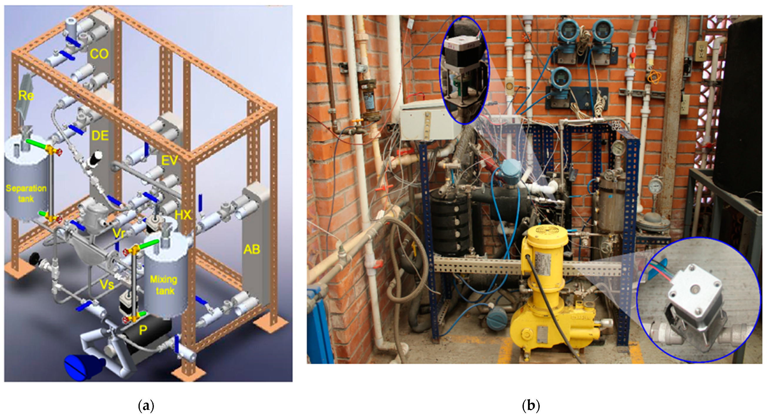
2.2. Experimental System

Figure 2a shows a diagram of the main mechanical components of the experimental SACS. Its support structure’s dimensions are length 1 m, width 0.8 m, and height 1 m, including the instrumentation for measurement and analysis. All components, including the pipes, valves, and accessories, are made of stainless steel to prevent corrosion. Five high efficiency plate heat exchangers were used, all of them oriented vertically; with 40 plates for DE, HX, and AB and 20 plates for CO and EV. Figure 2b shows a photograph of the experimental system.
In order to modify the solution load within the cooling system, two storage tanks of 4 L each were incorporated. The separation tank is placed at the outlet of DE; it allows that ammonia vapor to flow towards CO through the rectifier and the weak liquid solution to return to AB; the mixing tank receives the weak solution and the ammonia vapor from EV. Since the SACS is operated with the NH3-H2O working mixture, the rectifier used was a finned stainless steel tube, with a length of 40 cm and a nominal diameter of 1/2 inch, installed with 30° of inclination. To operate the equipment, a diaphragm, intermittent flow, or pulse pump was used, and a pulse damper had to be adapted, a small spherical chamber, and a membrane with nitrogen gas confined to the discharge pressure of the pump. There are two pressure levels (high and low) separated by two expansion valves. The first Vr was on the line from EV–CO, and the second on the line from DE–AB, both are unidirectional and made from stainless steel. Both are coupled to NEMA 17 DC stepper motors and allow us to maintain the position without using encoders.
For the experimental evaluation, a data acquisition system and external flow systems (a heating system, a cooling system, and a circuit of water to be chilled) were used. The auxiliary water heating system that the refrigeration system requires for its operation is installed on the roof of the Refrigeration and Heat Pumps Laboratory at IER-UNAM. It consists of a bank of evacuated tube collectors (18 modules divided into 3 sections connected in parallel) with a collection area of 30 m2. The system has a vertical storage tank and an auxiliary heater. The heated water is sent to the cooling system by means of a 0.33 HP pump. The cooling water for AB and CO is obtained from a cooling chiller (26–30 °C). For the analysis of the cooling power, water is circulated through the evaporator at constant temperature controlled by an electrical resistance.
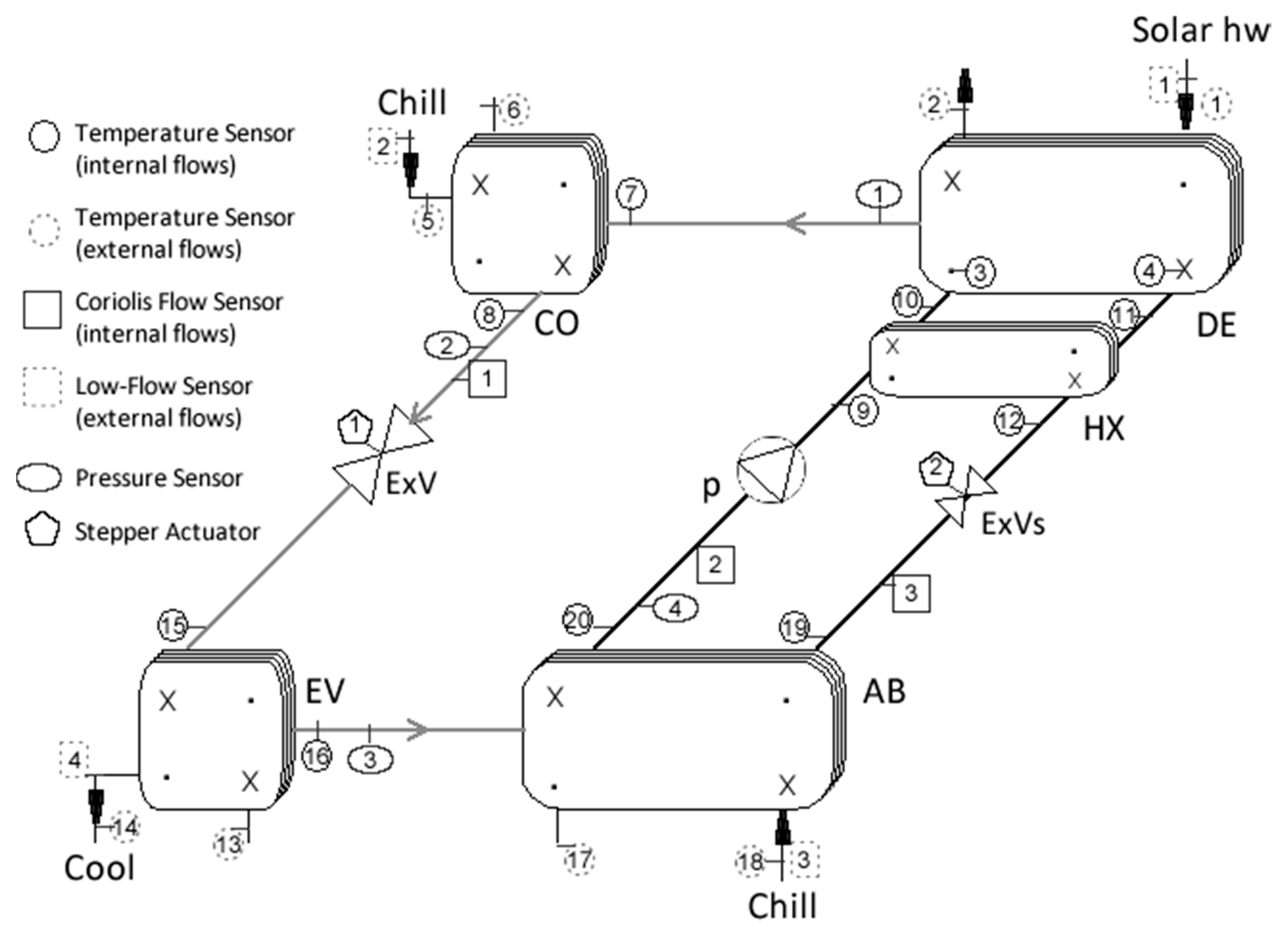
To evaluate the behavior of the SACS, it was necessary to measure some thermodynamic variables such as temperature, pressure, and mass flow of the weak and strong solution, cooling water (AB, CO), heating water (DE), and chilled water (EV). The variables were measured using electronic instruments: 20 RTD temperature sensors (PT1000) to register the flow temperatures at the inlet and outlet of each heat exchanger, 4 piezoelectric pressure transducers placed at the outputs of the DE, CO, EV, and AB; 3 Coriolis flowmeters, the first between the HX and AB heat exchanger for the weak solution, the second between the desorber and heat exchanger for the strong solution, the third between CO and EV and 4 rotameter-turbine flowmeters, at the inlets of external pressure flows. The location of each sensor in the SACS is shown in Figure 3.
Table 1 describes the accuracy of the sensors. For the data acquisition, a program was developed in which all the calibrated temperature, pressure, and mass flow sensors that were utilized in the system are included. The information is stored every twenty seconds in a database. A DAC 34972A with a multiplexer card and an input and output control card were used, the latter for the implementation of the PID. In Vr and Vs, the speed of both stepper motors can be controlled by means of a PMW signal and their direction with a digital signal using the micro-stepping motor driver A3967 and the Agilent card.

2.3. Dynamic System

The dynamic model of a refrigeration system proposed by Wen et al. [31] allows the comparison between the performance of an experimental control and the numerical simulations using MATLAB. The system basically contains 8 interconnected units: evaporator, absorber, desorber, condenser, heat exchanger, rectifier, pump, two throttle valves; two pressure levels were considered. For completeness, the main aspects of this model are here explained.
For each element of the system, pressure, temperature, and concentration are described, through a concentrated parameters approximation: according to the law of energy and conservation of mass; taking into account that the ammonia–water mixture phase changes throughout the cycle and the transfer of heat and mass are time-varying in the system; other assumptions are listed below:
  • Only two pressures are considered: high (desorber–condenser) and low (absorber-evaporator);
  • The thermal storage of the plates heat exchanger are neglected;
  • There is no pressure loss in the pipes;
  • The throttling process is isenthalpic;
  • Heat transfer to and from the surroundings are ignored;
  • The amount of work given to the pump is negligible;
  • The fluid leaves each component at the component temperature;
  • Constant heat exchanger efficiency.
The model in state space is as follows:
d M A B d t = m ˙ w e a k + m ˙ v , A B m ˙ s t r o n g
( M A B c p , s t r o n g ) d T A B   d t = m ˙ w e a k ( h w e a k , A B h s t r o n g ) + m ˙ v , A B ( h v , A B h s t r o n g ) Q ˙ A B
M A B d X s t r o n g d t = m ˙ w e a k X w e a k ( m ˙ w e a k + m ˙ v , A B ) X s t r o n g
d M c o h l , C O d t = m ˙ v , D E h v , D E m ˙ l , C O h l , C O Q ˙ C O
( M D E c p , w e a k ) d T D E   d t = m ˙ s t r o n g ( h s t r o n g , D E h w e a k ) + m ˙ v , D E ( h w e a k   h v , D E ) + Q ˙ D E
M D E d X w e a k d t = m ˙ s t r o n g X s r o n g + ( m ˙ v , D E m ˙ s t r o n g ) X w e a k
where M A B is the cumulative mass in the absorber, including the mass of refrigerant vapor and NH3 solution; m ˙ w e a k , m ˙ v , A B and m ˙ s t r o n g are the mass flow rates of the weak solution, refrigerant vapor, and strong solution, respectively. The mass traces and heat of the refrigerant vapor are imperceptible compared to those of the NH3 solution within the margin of error.
Therefore, M A B can approximately represent the mass of the NH3 solution in AB. h s t r o n g is the specific enthalpy of the solution at the AB outlet, h w e a k , A B is the specific enthalpy at the inlet of AB, h v , A B is the specific enthalpy of the heated refrigerant vapor in AB, and Q ˙ A B is the heat transfer rate from AB to the cooling water. T A B   is the average temperature, and c p , s t r o n g is the specific heat capacity of the solution in the case side of AB. M E V is the cumulative mass of the liquid refrigerant in the evaporator. T E V is the average temperature in EV, Q ˙ E V is the heat transfer rate from the chilled water to the evaporator, and h l , E V is the specific enthalpy of the liquid refrigerant under evaporating pressure.
If the volumes inside the pipes that join all parts of the system are neglected, the mass conservation equation of AB and the mass conservation equation in the whole system can be resolved as:
M D E X w e a k + M A B X s t r o n g = M N H 3
M D E + M C O + M E V + M A B = M t o t a l
The effectiveness of the heat exchanger given as [3]:
η s h e = T w e a k T w e a k . A B T w e a k T s t r o n g
The energy balance, therefore, leads to:
T s t r o n g ,   D E = T w e a k + m ˙ w e a k c p , w e a k m ˙ s t r o n g c p , s t r o n g   ( T w e a k T s t r o n g )
The heat transfer rate can be calculated by taking the desorber as an example:
Q ˙ D E = m ˙ h o t   w c p , w ( T h o t   w , i T h o t   w , o )
Q ˙ D E = ( U A ) D E   ( T h o t   w , i T D E ) ( T h o t   w , o T D E ) ln ( ( T h o t   w , i T D E ) ( T h o t   w , o T D E ) )
Connecting Equations (16) and (17), the heat transfer rate in the DE and the hot water outlet temperature can be estimated:
Q ˙ D E = m ˙ h o t   w c p , w ( 1 e ( U A ) D E / m ˙ h o t   w c p , w ) ( T h o t   w , i T D E )
T h o t   w , o = T h o t   w , i ( 1 e ( U A ) D E / m ˙ h o t   w c p , w ) ( T h o t   w , i T D E )  
Analogous results can also be concluded for the other main components.
The mass flow rate of the strong solution from AB is defined by the solution pump, and it can be defined as:
m ˙ s t r o n g = k ρ s t r o n g f p V p
where the coefficient k is particular to the pump; ρ s t r o n g is the strong solution density; f p is the frequency driving the solution pump; V p is the internal volume of the pump. The valves Vr and Vs are adiabatic devices. The mass flow rate can be calculated as:
m ˙ l = A v l C v l ρ l ( Δ P + ρ l g ( Z + z ) )
where C v l is the valve flow coefficient; Δ P is the pressure difference between the connected components; g is the gravitational acceleration; ρ is the density. By controlling the valve aperture, the cross-section area A v l   can be set, and this can be used as a manipulated variable for controlling the mass flow rates in the SACS [47,48].
The state of the SACS can be described by six variables: the cumulative mass in AB ( M A B ) , the average temperature in AB ( T A B ), the concentration of the strong solution in AB ( X s t r o n g ) , the cumulative mass in EV ( M E V ), the average temperature in DE ( T D E ), and the concentration of the weak solution in DE ( X w e a k ) .
SACS model can be written in state-space form x ˙ = f ( x ,   u ,   θ , p ) with the following state vector:
x = [ M A B   T A B   X w e a k   M E V   T A B   X s t r o n g   ] T
The input vector for the model is:
u = [ m ˙ h o t   w   m ˙ c o o l   w   m ˙ c h i l l   w T c o o l   w , i   T h o t   w , i   f p   ] T
where m ˙ h o t   w   m ˙ c o o l   w   m ˙ c h i l l   w   T h o t   w , i   T c o o l   w , i   f p are the external water circuits mass flow rates and inlet temperatures. θ ( t ) is an internal variables vector that depends on the state, and p is a constant value parameters vector.
[ M ˙ A B T ˙ A B X ˙ s t r o n g M ˙ C O T ˙ D E X ˙ w e a k ] = [ m ˙ w e a k + m ˙ v , A B m ˙ s t r o n g ( m ˙ w e a k ( h w e a k , A B h s t r o n g ) + m ˙ v , A B ( h v , A B h s t r o n g ) Q ˙ A B ) / ( M A B C p , s t r o n g ) ( m ˙ w e a k X w e a k ( m ˙ s t r o n g m ˙ v , A B ) X s t r o n g ) / M A B Q ˙ C O / m ˙ v , D E h v , D E m ˙ l , c h l , c ( m ˙ s t r o n g ( h s t r o n g , D E h w e a k ) + m ˙ v , D E ( h v , D E h w e a k ) + Q ˙ D E ) / ( M D E C p , w e a k ) m ˙ s t r o n g X s t r o n g ( m ˙ w e a k m ˙ v , D E ) X w e a k ]

3. Control System

3.1. PID Control

Flow control is the most suitable manipulated variable for the feedback control loops. Flow controllers have been tuned empirically with proportional gains less than unity and quick integral times. The processes dynamics are due to compressibility or inertial effects; most of the perturbances are high-frequency noise (periodic or random) because of turbulence, valve changes, and pump vibration. Usually limits of stability in the gain of the controller are reached, due to the time delays and thermal capacitances that are inherent in the system.
Temperature controllers are usually proportional–integral–derivative (PID), which manipulate the flow of fuel or steam to a heating system operated in proportion to the rate of heat. This is because the heat of condensation of the steam, and the heating value of the fuel is usually not affected by load. On the other hand, when the cooling water or hot oil is the manipulated variable, the heat rate is highly non-linear, mostly because the heat transfer rate requires that the outlet utility temperature approaches the inlet temperature when the rate of heat transfer increases.
Usually, a closed-loop system has as its control objective, in principle, the regulation of the set point (SP), represented by r (t). This implies, in general terms, that each control loop manages to maintain the process variable (PV), represented as y (t), close to the SP, despite disturbances [49]. The PID algorithm is undoubtedly the most widely implemented in industrial applications. A PID controller is composed of the sum of a proportional action, an integral action, and a derivative action. The ideal PID controller equation can be written as follows:
u ( t ) = K ( e ( t ) + 1 T i 0 t e ( τ ) d τ + T d d e ( t ) d t )
where u(t) represents the control variable; e(t) is the error between what is measured and what is desired. The controller parameters are the proportional gain K, the integral time T i , and the derivative time T d .

3.2. PID Setup

Figure 4 shows a scheme of the feedback control loops. The objective is to maintain the cooled water temperature in the evaporator at TSP. The process variable in this first control loop is the measured temperature y3; its difference is the error e3. On the other hand, flow m ˙ l c o is the measured process variable y1 of a cascaded control loop, whose set point y1 SP is determined by a model-based relationship between the temperature error e3 and the desired flow of refrigerant from CO to EV (in the figure shown as the manual control (MC) block). Another control loop is needed in the weak solution circuit between DE and AB to ensure that increasing the flow in the strong solution circuit is compensated by a decrease in the mass flow between DE and AB, which comprises the process variable y2. Therefore, the objective of this control loop is to maintain the sum (y1 + y2) at a constant value yp, the mass flow of strong solution induced by the solution pump p (see Equation (20)).
This approach to control the SACS configuration is based on experimental conclusions. For the experimental assessment, Table 2 shows the parameters values. NH3 concentration (Xstrong = 0.40) was calculated for the ammonia–water fluid pair method proposed by Tillner-Roth [50].

4. Results

4.1. Parametric Evaluation of the Experimental System

This section presents the system performance; the behavior or trend is determined to define parameters and evaluate a desired characteristic of the system. In addition to the selection of directly sensed variables, calculated parameters have been selected for the SACS assessment. Experimental tests were carried out to validate repeatability. The measuring range for the parameters are detailed in Table 2. The high-temperature water provided to the system by the solar collectors was between 98 and 110 °C, and the cooling water temperatures were in the range 26–30 °C; they extracted thermal energy from the condenser and the absorber in a serial circuit fed with cooling water starting at AB, so AB and CO inlet temperatures are assumed equal.
Figure 5 shows the behavior of the system pressures for a characteristic test: high (CO, DE) and low (EV, AB). Hot water was supplied to the system from 95 to 110 °C, which means 86 to 98 °C in the internal solution mixture; the cooling water used to extract the thermal energy in AB and CO was provided at 26, 28, and 30 °C. The system operated in steady-state conditions and was manually tuned.
Figure 6 shows the external (a) and internal (b) evaporator cooling powers (QEV) varying the heating temperature supplied to the desorber and for different cooling water inlet temperatures at CO and AB. The maximum cooling capacity obtained is 3.86 kW external and 4.87 kW internal at 95 °C hot water, 86 °C solution temperature at DE, and 26 °C cooling water in CO.
For three different cooling water temperatures, Figure 7a shows the evaporation temperature variation as the solution temperature at DE is increased. For a generation temperature approximated to 86 °C and a condensation temperature of 30 °C, the refrigerant mass flow rate was unsteady, so, in order to keep it constant, it was necessary either to increase the heating water temperature or decrease the cooling water temperature. Figure 7b shows the external COP registered at the same conditions. From this figure, it is evident that the refrigerant desorption is lower as well as the generation temperature is increased, which affects the COP achieved by the SACS.
The uncertainty is the associated parameter to the measurement result that characterizes the dispersion of the values attributed to the measuring device [51]. An analysis of type A uncertainty was implemented on the experimental data [52,53], in view of the technical specifications of the instruments required, cf. Table 1; ±0.031 °C was calculated for the temperature measurements, ±0.067 bar for pressure, ±0.020 kg/min for external flows, and ±0.006 kg/min for internal flows; ±0.038 and ±0.015 kW for internal and external cooling load; 0.071 for COP.

4.2. Dynamic Model

Design and experimental parameters of the SACS are listed in Table 3 and Table 4.
The comparison of the simulated model response and the experimental measured output for the same output signal is shown in Figure 8. The results show that the model fits the data absolute average deviation (A.A.D%) of 4.28.
The information is stored every twenty seconds in a database, and every experiment was completed in around two hours. The recorded mass flow rates, temperatures, and pressures were described as inputs of the model simulation. The refrigerant temperature at the exit of the evaporator was compared to the model simulation results under the same references, while the experimental data ranges analyzed were registered, the mass flow rate of the hot water on the storage tank, the chilled water, and cooled water were kept constant until the next range was analyzed.

4.3. PID Control

For calibrating the gains of the PID controller, Nichols and Ziegler’s open-loop tuning techniques were followed using the simulation model (Table 5); having the ultimate gain and frequency, the parameters of Table 3 can be obtained. Figure 9 and Figure 10 show a good agreement between simulation and experiment. In the simulation, constant parameters were assumed. Several experimental limitations have already been described throughout this text, and thus, a direct comparison is not feasible. However, the simulation trends can be related and compared qualitatively to those of the experiment. According to this purpose, the experimental tests are only compared with each other. Even so, correction measures have been applied to the experimental parameters for the comparison of the experimental test and the calculation of the COP.

5. Discussion

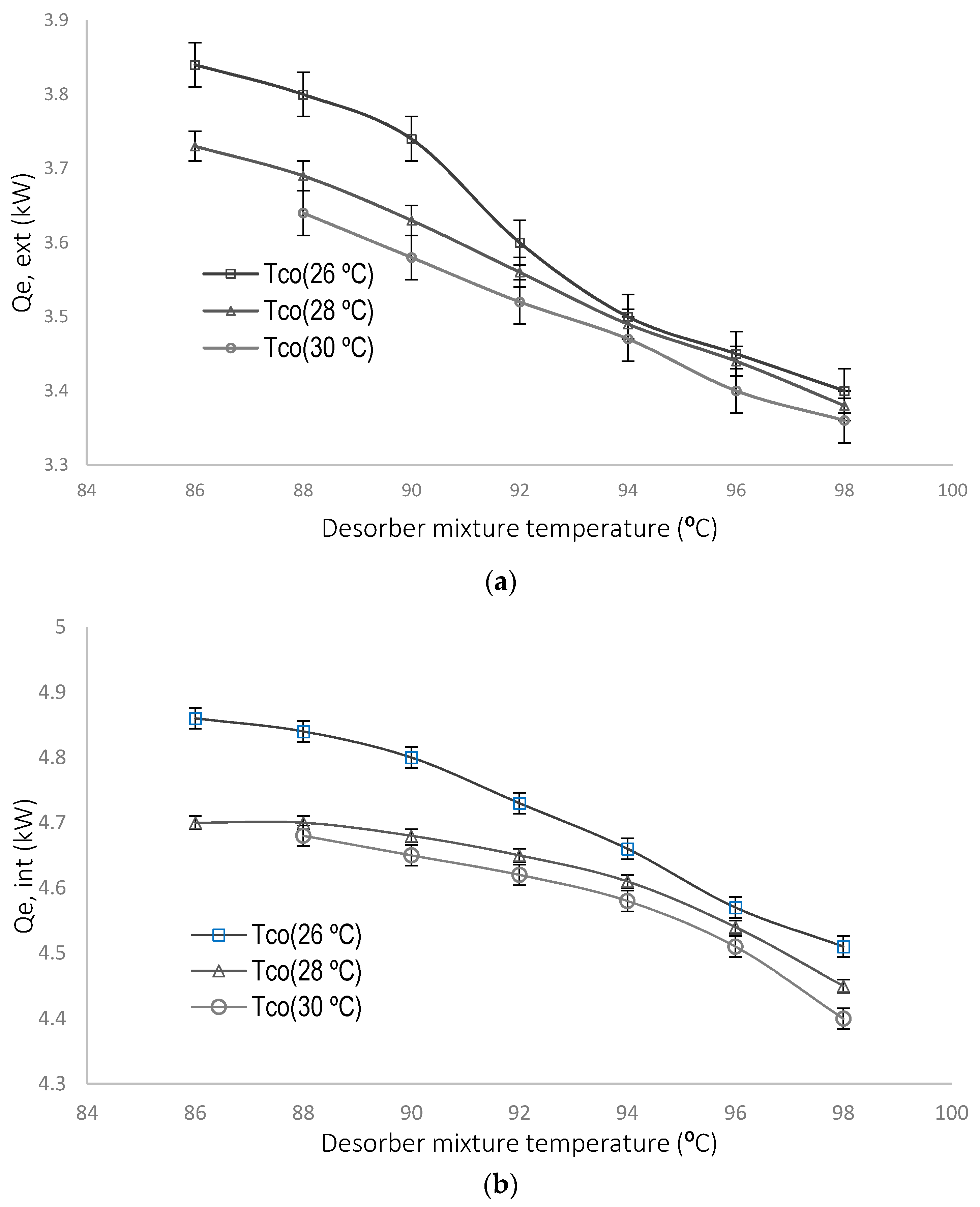
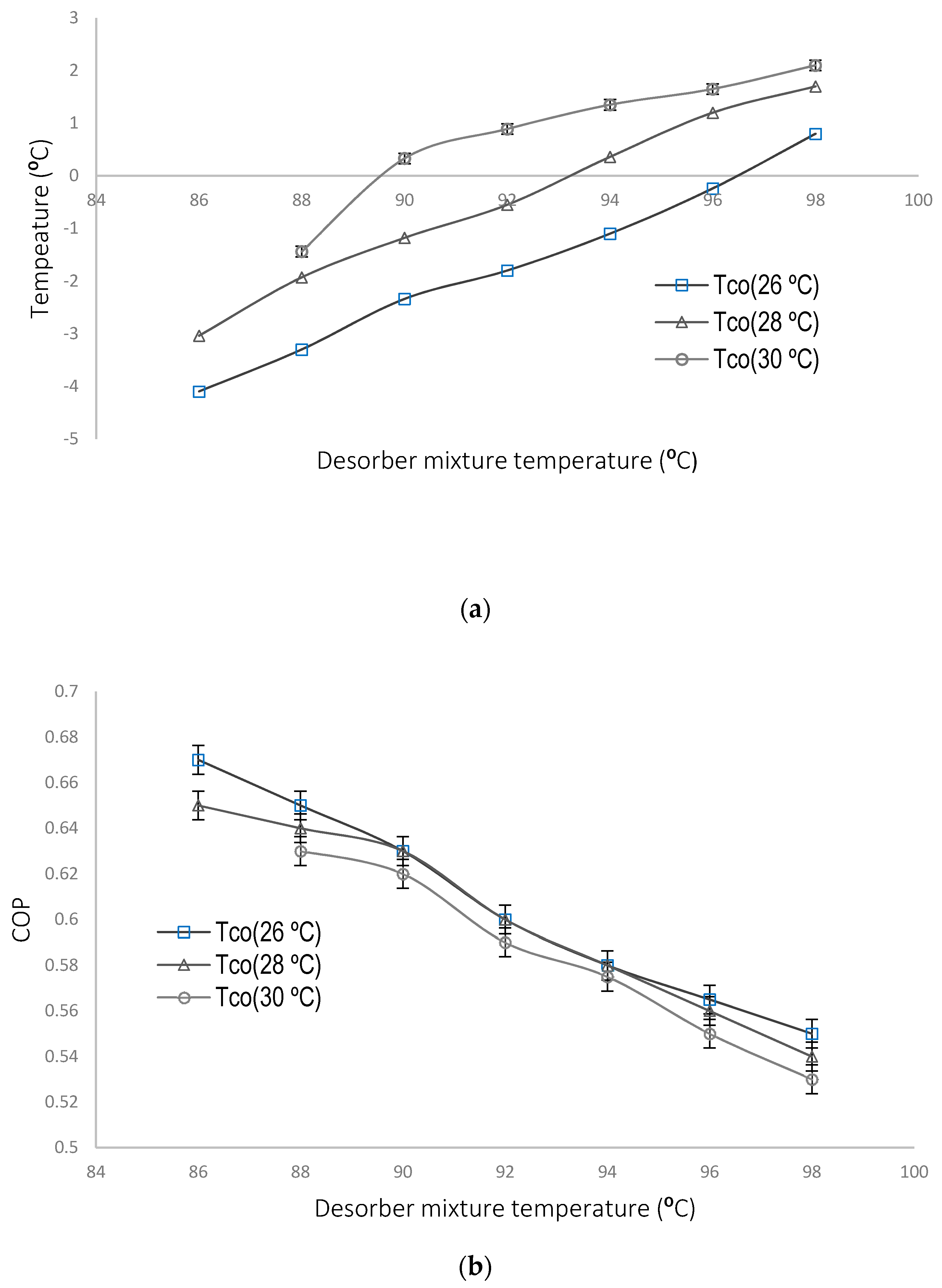
Several experimental tests were carried out to validate the repeatability of the parametric evaluation, at the beginning, for a non-controlled system. The operating conditions and the solution flow influence determined the following methodology for stability control: first, it was developed an object oriented program through a data acquisition system, then, some test runs were carried out to finally be able to validate the proposed controller. The maximum cooling capacity obtained was 3.86 kW external and 4.87 kW internal; this was obtained at 95 °C hot water, 86 °C solution temperature at DE, and 26 °C cooling water in CO. As expected, the best cooling capacity was achieved at the lowest cooling water temperatures in the condenser, and the best COP achieved was 0.67 with an average of 0.58.
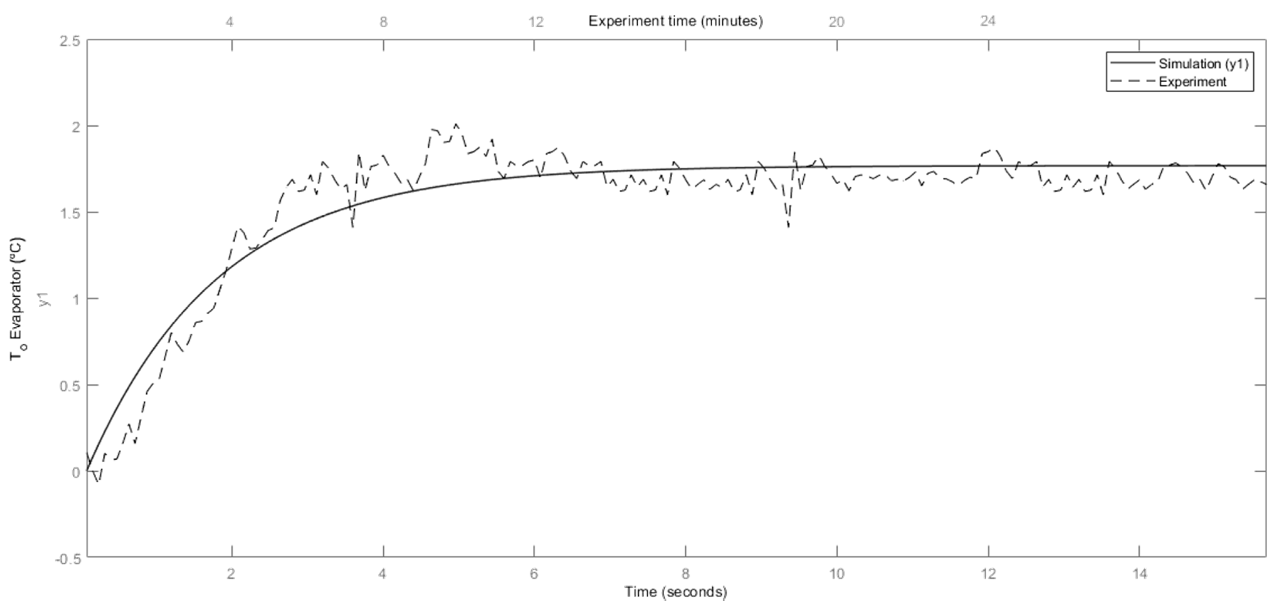
The validation of the dynamic simplified model was implemented in MATLAB/Simulink, and its accuracy was verified. The thermodynamic properties for the ammonia–water solution with an ammonia concentration of 40% for the temperatures, at which the system was operated, were obtained by the Tillner-Roth [51] equations. The comparison results shown in Figure 8 show good agreement between the simulated and experimental data, which is a good reference to validate the experimental PID controllers proposed in the system.
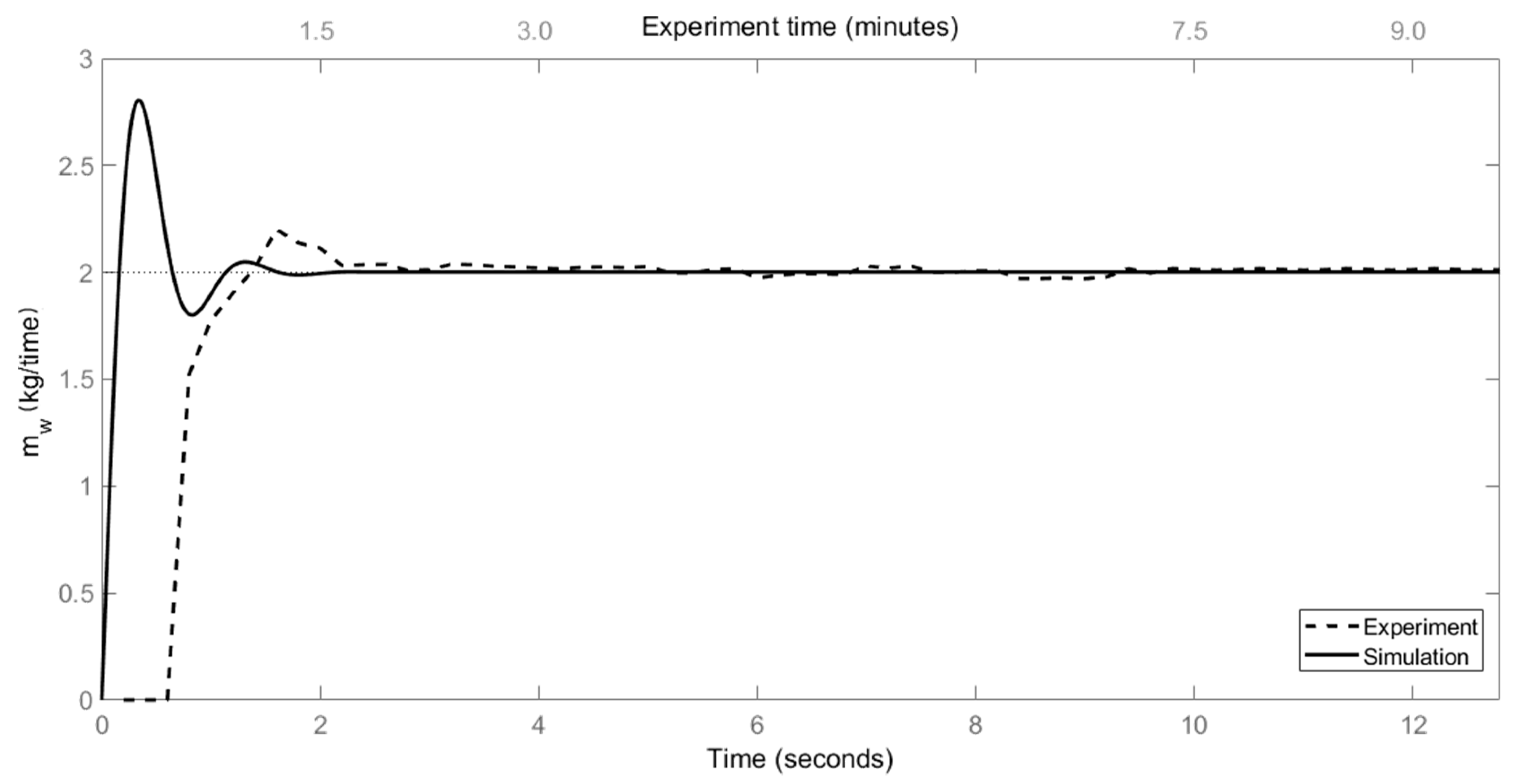
The feasibility of the PID control for the SACS began with local experimental tests of the behavior of the equipment operated with a PID tuning with known techniques from Ziegler and Nichols; then, a linearized model was used to compare the practical results. The hypothesis was that the control of the refrigerant and diluted solution mass flows, in addition to maintaining the levels in the mixing and separation tanks, could achieve the stability and control of the system. It was then possible to improve other parameters such as evaporator cooling capacity and COP. Response time, beyond the inherent advantages of automation, has been reduced; once the transitory part is reached, the range of the control objective is maintained indefinitely. The operation proposal of cascaded PID’s was also verified. The simulation results show good agreement with the experimental data, except for parts of the initial transient response.
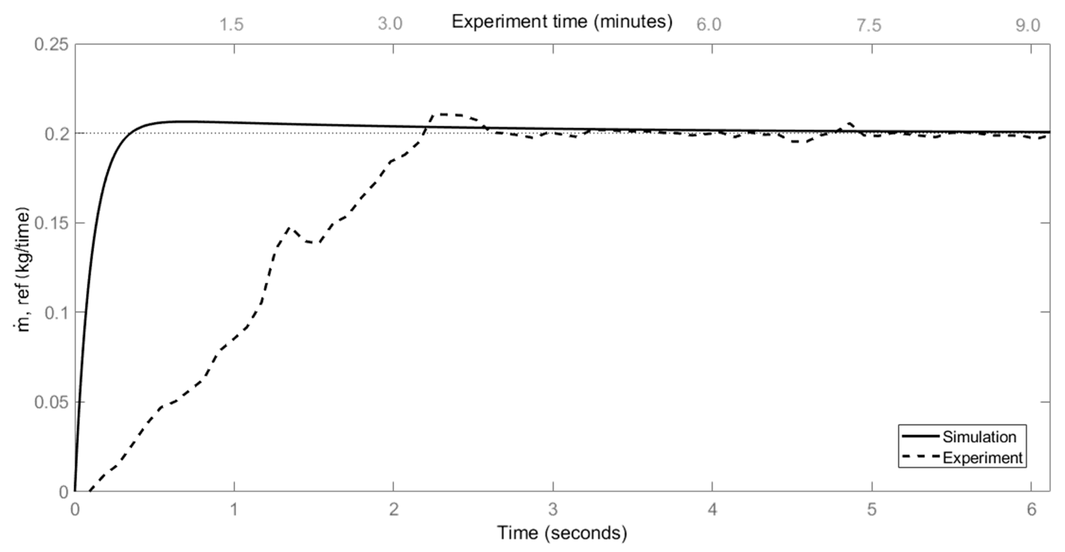
On the validation of the control proposal, the adaptation of the dynamic model exposed in state space is proposed. The thermodynamic and control results in the SACS were analyzed with MATLAB and compared to the experimental results in the real SACS, considering an NH3-H2O mixture with a strong concentration of 0.40. The traditional PID controller action is augmented with a version of two cascaded PID’s, which overcomes several issues of previous formulations. There are linear alternatives that attempt to approximate the behavior of non-linear techniques but reduce their complexity. As PID control strategies, in this type of control, the main purpose is to simplify controllers designed for specific operation points and some rules that allow switching between them or operated in parallel. Except for the transitory behavior data, the model simulated data in the settlement time and the experimental results were concurrent with a variation of ±2%.

6. Conclusions

This investigation aims to present a proposal for automatic control in the SACS resulting from a black box analysis from which the tuning of the PID controller gain follows. This study has made it possible to advance in the operation of the system, improving the performance of the equipment operating without control, achieving, on average, cooling powers of 3.8 kW, external COP of 0.58, and −4.1 ° C evaporator cooling temperature at a desorber temperature of 86 °C and condenser temperature of 26 °C. Furthermore, shorter transient times are obtained, compared to the usual response of 3–5 min, as well as longer stand-alone stable times, which is desirable in this sort of cooling systems.
A theoretical model was developed to reproduce the theoretical behavior of an ideal cascade PID controller of the SACS, for the evaporation temperature variable, manipulating the variables of mass flow of weak solution (PID1) and mass flow of refrigerant (PID2), operating in parallel; this was validated with data from experimental tests. Obtaining an average difference between 8% for the solution case and 10% for the refrigerant case.
The transient response time to reach the steady state and the SP of the PID was 2 min for the weak solution flow and 5 min for the refrigerant flow. The temperature objective was reached in 11 min. Once the settling time had been reached, the coupled PID controllers maintained the conditions with a variation error of ±2% during the entire operating time of the system. The system fulfilled what was expected, so it is concluded that it is a viable technical and economic proposal for absorption systems of various capacities.

Author Contributions

Conceptualization, Y.G., R.B., W.R. and A.V.; methodology, Y.G., R.B., W.R., A.V. and V.H.G.; software, Y.G., V.H.G. and J.C.J.-G.; validation, Y.G., R.B., W.R., A.V. and V.H.G.; formal analysis, Y.G., R.B., W.R., A.V. and V.H.G.; investigation, Y.G., A.V. and V.H.G.; resources, Y.G., R.B., W.R., V.H.G., A.V. and J.C.J.-G.; data curation, Y.G. and V.H.G.; writing—original draft preparation, Y.G., V.H.G. and A.V.; writing—review and editing, Y.G., R.B., A.V., V.H.G., J.C.J.-G. and W.R.; visualization, Y.G., R.B., A.V., V.H.G., J.C.J.-G. and W.R.; supervision, R.B., A.V., V.H.G., J.C.J.-G. and W.R.; project administration, Y.G., R.B., A.V., V.H.G., J.C.J.-G. and W.R.; funding acquisition, Y.G., R.B., A.V., V.H.G., J.C.J.-G. and W.R. All authors have read and agreed to the published version of the manuscript.

Funding

The project was also partially funded by DGAPA-UNAM project PAPIIT IN1109119.

Institutional Review Board Statement

Not applicable.

Informed Consent Statement

Not applicable.

Data Availability Statement

PAPIME PE107121.

Acknowledgments

The experiments described in this paper were carried out within the project.

Conflicts of Interest

The authors declare no conflict of interest.

Nomenclature

Aeffective area in contact (m2)
A v l minimum cross-section area (m2)
ABabsorber
COcondenser
COPcoefficient of performance
Cpspecific heat at constant pressure (kJ/kg–K)
C v l flow coefficient of the valve
DEdesorber
EVevaporator
FRflow ratio
HXheat exchanger
Hspecific enthalpy (kJ/kg)
m ˙ mass flow (kg/min)
Mmass (kg)
Psolution pump
Q ˙ heat rate (kW)
Rrefrigeration
RErectifier
Ttemperature (°C)
Ttime (s)
Uheat transfer coefficient (kW/m2K)
UAglobal thermal surface conductivity (kW/K)
Vrrefrigerant expansion throttle valve
Vssolution expansion throttle valve
Wpower (kW)
Xconcentration of the NH3H2O solution
Zheight difference between the upper component outlet and lower component inlet
Zproportion level height of liquid in the upper component to the accumulative mass
Subscript:
0ambience
chill wchilled water
cool wcooling water
hot shot solution
hot whot water
i, oinlet, outlet
lliquid phase
maxmaximum
ppump
rrefrigerant
ssolution
strongstrong solution
vvapor phase
vlvalve
weakweak solution

References

  1. IEA-Cooling. Tracking Report-June 2020. Available online: https://www.iea.org/reports/cooling (accessed on 1 June 2021).
  2. Kalkan, N.; Young, E.A.; Celiktas, A. Solar thermal air conditioning technology reducing the footprint of solar thermal air conditioning. Renew. Sust. Energy Rev. 2012, 16, 6352–6383. [Google Scholar] [CrossRef]
  3. Joudi, K.A.; Lafta, A.H. Simulation of a simple absorption refrigeration system. Energy Convers. Manag. 2001, 42, 1575–1605. [Google Scholar] [CrossRef]
  4. Ziegler, F. Recent developments and future prospects of sorption heat pump systems. Int. J. Therm. Sci. 1999, 38, 191–208. [Google Scholar] [CrossRef]
  5. Ziegler, F.; Alefeld, G. Coefficient of performance of multistage absorption cycles. Int. J. Refrig. 1987, 10, 285–295. [Google Scholar] [CrossRef]
  6. Ziegler, J.G.; Nichols, N.B. Optimum settings for automatic controllers. Math. Comput. Sci. 1942, 64, 759–768. [Google Scholar] [CrossRef]
  7. Labus, J.M.; Bruno, C.J.; Coronas, A. Review on absorption technology with emphasis on small capacity absorption machines. J. Therm. Sci. Eng. Appl. 2013, 17, 739–762. [Google Scholar] [CrossRef]
  8. Abed, A.M.; Alghoul, M.A.; Sopiana, K.; Majdi, H.S.; Al-Shamani, A.N.; Muftah, A.F. Enhancement aspects of single stage absorption cooling cycle: A detailed review. Renew. Sust. Energy Rev. 2017, 77, 1010–1045. [Google Scholar] [CrossRef]
  9. Srikhirin, P.; Aphornratana, S.; Chungpaibulpatana, S. A review of absorption refrigeration technologies. Renew. Sust. Energy Rev. 2001, 5, 343–372. [Google Scholar] [CrossRef]
  10. Dincer, I.; Midilli, A.; Hepbasli, A.; Karakoc, T.H. Global Warming: Engineering Solutions; Springer: Boston, MA, USA, 2010; pp. 147–159. [Google Scholar]
  11. Dincer, I.; Dost, D. A simple model for heat and mass transfer in absorption cooling systems (ACSs). Int. J. Energy Res. 1996, 20, 237–243. [Google Scholar] [CrossRef]
  12. Ng, K.C.; Chua, H.T.; Han, Q.; Kashiwagi, T.; Akisawa, A.; Tsurusawa, T. Thermodynamic Modeling of Absorption Chiller and Comparison with Experiments. Heat Transf. Eng. 1999, 20, 42–51. [Google Scholar]
  13. Sterner, D.; Sunden, B. Performance of plate heat exchangers for evaporation of ammonia. Heat Transf. Eng. 2006, 27, 45–55. [Google Scholar] [CrossRef]
  14. Goodarzi, M.; Amiri, A.; Mohammad, S.G.; Mohammad, R.S.; Kirimipour, A.; Languri, E.M.; Dahari, M. Investigation of heat transfer and pressure drop of a counter flow corrugated plate heat exchanger using MWCNT based nanofluids. Int. Commun. Heat Mass Transf. 2015, 66, 172–179. [Google Scholar] [CrossRef]
  15. Evola, G.; Le Pierrès, N.; Boudehenn, F.; Papillon, P. Proposal and validation of a model for the dynamic simulation of a solar-assisted single-stage LiBr/water absorption chiller. Int. J. Refrig. 2013, 36, 1015–1028. [Google Scholar] [CrossRef]
  16. Kim, B.; Park, J. Dynamic simulation of a single-effect ammonia-water absorption chiller. Int. J. Refrig. 2007, 30, 535–545. [Google Scholar] [CrossRef]
  17. Ruz, M.L.; Garrido, J.; Vázquez, F.; Morilla, F. A hybrid modeling approach for steady-state optimal operation of vapor compression refrigeration cycles. Appl. Therm. Eng. 2017, 120, 74–87. [Google Scholar] [CrossRef] [Green Version]
  18. Kim, D.S.; Infante Ferreira, C.A. Analytic modelling of steady state-single effect absorption cycles. Int. J. Refrig. 2008, 31, 1012–1020. [Google Scholar] [CrossRef]
  19. Cai, W.; Sen, M.; Paolucci, S. Dynamic simulation of an ammonia-water absorption refrigeration system. Ind. Eng. Chem. Res. 2011, 51, 2070–2076. [Google Scholar] [CrossRef]
  20. Viswanathan, V.K.; Rattner, A.S.; Determan, M.D.; Garimella, S. Dynamic model for a small-capacity ammonia-water absorption chiller. HVACR Res. 2013, 19, 865–881. [Google Scholar] [CrossRef]
  21. Martinho, L.C.S.; Vargas, J.V.C.; Balmant, W.; Ordonez, J.C. A single stage absorption refrigeration system dynamic mathematical modeling, adjustment and experimental validation. Int. J. Refrig. 2016, 68, 130–144. [Google Scholar] [CrossRef]
  22. Iranmanesh, A.; Mehrabian, A.M. Dynamic simulation of a single-effect LiBr-H2O absorption refrigeration cycle considering the effects of thermal masses. Energy Build. 2013, 60, 47–59. [Google Scholar] [CrossRef]
  23. Ochoa, A.A.V.; Dutra, J.C.C.; Henríquez, J.R.G.; dos Santos, C.A.C. Dynamic study of a single effect absorption chiller using the pair LiBr/H2O. Energy Convers. Manag. 2016, 108, 30–42. [Google Scholar] [CrossRef]
  24. Kohlenbach, P.; Ziegler, F. A dynamic simulation model for transient absorption chiller performance. Part II: Numerical results and experimental verification. Int. J. Refrig. 2008, 31, 226–233. [Google Scholar] [CrossRef]
  25. Puig-Arnavat, M.; López-Villada, J.; Bruno, J.C.; Coronas, A. Analysis and parameter identification for characteristic equations of single- and double-effect absorption chillers by means of multivariable regression. Int. J. Refrig. 2010, 33, 70–78. [Google Scholar] [CrossRef]
  26. Albers, J.; Kühn, A.; Petersen, S.; Ziegler, F. Control of Absorption Chillers by Insight: The characteristic equation. Czas. Tech. Mech. 2008, 105, 3–12. [Google Scholar]
  27. Albers, J. New absorption chiller and control strategy for the solar assisted cooling system at the German federal environment agency. Int. J. Refrig. 2014, 39, 48–56. [Google Scholar] [CrossRef]
  28. Matsushima, H.; Fujii, T.; Komatsu, T.; Nishiguchi, A. Dynamic simulation program with object-oriented formulation for absorption chillers (modelling, verification, and application to triple-effect absorption chiller). Int. J. Refrig. 2010, 33, 259–268. [Google Scholar] [CrossRef]
  29. Yao, Y.; Huang, M.; Chen, J. State-space model for dynamic behavior of vapor compression liquid chiller. Int. J. Refrig. 2013, 36, 2128–2147. [Google Scholar] [CrossRef]
  30. Osta-Omar, S.M.; Micallef, C. Mathematical Model of a Lithium-Bromide/Water Absorption Refrigeration System Equipped with and Adiabatic Absorber. Computation 2016, 4, 44. [Google Scholar] [CrossRef] [Green Version]
  31. Wen, H.; Wu, A.; Liu, Z.; Shang, Y. A State-Space Model for Dynamic Simulation of a Single-Effect LiBr/H2O Absorption Chiller. IEEE Access 2019, 7, 57251–57258. [Google Scholar] [CrossRef]
  32. Fernández-Seara, J.; Vázquez, M. Study and control of the optimal generation temperature in NH3-H2O absorption refrigeration system. Appl. Therm. Eng. 2001, 21, 343–357. [Google Scholar] [CrossRef]
  33. Rêgo, A.T.; Hanriot, S.M.; Oliveira, A.F.; Brito, P.; Rêgo, T.F.U. Automotive exhaust gas flow control for an ammonia-water absorption refrigeration system. Appl. Therm. Eng. 2014, 64, 101–107. [Google Scholar] [CrossRef]
  34. Jeong, A.S.; Younggy, S.; Chung, J.D. Dynamics and control of solution levels in a high temperature generator for an absorption chiller. Int. J. Refrig. 2012, 35, 1123–1129. [Google Scholar]
  35. Güido, W.H.; Lanser, W.; Petersen, S.; Ziegler, F. Performance of absorption chillers in field test. Appl. Therm. Eng. 2018, 134, 353–359. [Google Scholar] [CrossRef]
  36. Bennet, S. The Past of PID Controllers. Annu. Rev. Control 2001, 25, 43–53. [Google Scholar] [CrossRef]
  37. Björn, N.; Dalibard, A.; Schnabel, L.; Eicker, U. Approaches for the optimized control of solar thermally driven cooling systems. Appl. Energy 2017, 185, 732–744. [Google Scholar]
  38. Sabbagh, A.A.; Gómez, J.M. Optimal control of single stage LiBr/water absorption chiller. Int. J. Refrig. 2018, 92, 1–9. [Google Scholar] [CrossRef]
  39. Hamid, N.; Kamal, M.; Yahaya, F.H. Application of PID controller in controlling refrigerator temperature. In Proceedings of the 2009 5th International Colloquium on Signal Processing & Its Applications, Kuala Lumpur, Malaysia, 6–8 March 2009; Volume 1, pp. 378–384. [Google Scholar]
  40. Salazar, M.; Méndez, F. PID control for a single-stage transcritical CO2 refrigeration cycle. Appl. Therm. Eng. 2014, 67, 429–438. [Google Scholar] [CrossRef]
  41. Bejarano, G.; Alfaya, J.A.; Rodriguez, D.; Morilla, F.; Ortega, M.G. Benchmark for PID control of Refrigeration Systems based on Vapour Compression. IFAC Pap. 2018, 51, 497–502. [Google Scholar] [CrossRef]
  42. Zadeh, L.A. Fuzzy Sets. Inf. Control 1965, 8, 338–353. [Google Scholar] [CrossRef] [Green Version]
  43. Visek, E.; Mazzrella, L.; Motta, M. Performance Analysis of a Solar Cooling System Using Self-Tuning Fuzzy-PID Control with TRNSYS. Energy Procedia 2014, 57, 2609–2618. [Google Scholar] [CrossRef] [Green Version]
  44. Lima, K.C.; Caldas, A.M.A.; dos Santos, C.A.C.; Ochoa, A.A.V.; Dutra, J.C.C. Flow Control For Absorption Chillers Using the Par LiBr/H2O Driven in Recirculation Pumps of Low Power. IEEE Access 2016, 14, 1624–1629. [Google Scholar] [CrossRef]
  45. Vinther, K.; Nielsen, R.J.; Nielsen, K.M.; Andersen, P.; Pedersen, T.S.; Bendtsen, J.D. Absorption Cycle Heat Pump Model for Control Design. In Proceedings of the 2015 European Control Conference (ECC), Linz, Austria, 15–17 July 2015. [Google Scholar]
  46. Jiménez-García, J.C.; Rivera, W. Parametric analysis on the experimental performance of an ammonia/water absorption cooling system built with plate heat exchangers. Appl. Therm. Eng. 2019, 148, 87–95. [Google Scholar] [CrossRef]
  47. Hewitt, N.J.; Mcmullan, J.T.; Murphy, N.E.; Ng, C.T. Comparison of expansion valve performance. Int. J. Energy Res. 1995, 19, 347–359. [Google Scholar] [CrossRef]
  48. Tassou, S.A.; Al-Nizari, H.O. Investigation of the effects of thermostatic and electronic expansion valves on the steady-state and transient performance of commercial chillers. Int. J. Refrig. 1993, 16, 49–56. [Google Scholar] [CrossRef]
  49. Shinskey, F.G. Process Control Systems: Application, Design, and Tuning, 4th ed.; McGraw-Hill Inc.: New York, NY, USA, 1996; pp. 74–79. [Google Scholar]
  50. Tillner-Roth, R.; Friend, D.G. A Helmholtz Free Energy Formulation of the Thermodynamic Properties of the Mixture {Water + Ammonia}. J. Phys. Chem. Ref. Data 1998, 27, 63–96. [Google Scholar] [CrossRef] [Green Version]
  51. Iso GUM. Guide to the Expression of Uncertainty in Measurementm; ISO: Geneva, Switzerland, 2008. [Google Scholar]
  52. Moffat, R.J. Using Uncertainty Analysis in the Planning of an Experiment. J. Fluids Eng. 1985, 107, 173–178. [Google Scholar] [CrossRef]
  53. Moffat, R.J. Contributions to the Theory of Single-Sample Uncertainty Analysis. J. Fluids Eng. 1982, 104, 250–258. [Google Scholar] [CrossRef] [Green Version]
Figure 1. (a) Absorption cooling cycle. (b) Experimental diagram of the absorption cooling cycle. Colors indicate the correspondences of the components.
Energies 14 04058 g001aEnergies 14 04058 g001b
Figure 2. (a) Layout of experimental SACS design. (b) Real experimental SACS setup; insets show the stepper motors for controlling the expansions valves.
Energies 14 04058 g002
Figure 3. Sensors and actuators in the SACS.
Energies 14 04058 g003
Figure 4. Block diagram of a cascade PID feedback loop applied on the SACS.
Energies 14 04058 g004
Figure 5. Main pressure profile in the DE and EV system at different TCO and TDE.
Energies 14 04058 g005
Figure 6. External (a) and internal (b) evaporator cooling capacity as a function of the heating water temperature at DE for different cooling water temperatures.
Energies 14 04058 g006
Figure 7. (a) Evaporator temperatures by heating solution temperatures at different TCO and internal (b) COP versus heating solution temperatures at different TCO.
Energies 14 04058 g007
Figure 8. Comparison of temperature response model simulation data (solid line) and experimental data (dashed line).
Energies 14 04058 g008
Figure 9. Response of the weak solution valve with PID1.
Energies 14 04058 g009
Figure 10. Response of the expansion valve with PID2.
Energies 14 04058 g010
Table 1. Sensors summary data.
VariableMeasuring InstrumentOperation RangeAccuracy
FlowCoriolis flow meter0 to 20 (kg/min)±0.1%
Impeller flow meter0 to 60 (kg/min)±1%
PressurePressure transductor0 to 25 (bar)±1%
TemperatureRTD temperature−40 a 750 (°C)±0.3 °C
Table 2. Range of operating conditions of the thermal units.
Parameters UnitsExperimental Value
Pressures
Desorberbar11–15
Condenserbar10–14
Evaporatorbar2–4
Absorberbar2–3
Flow rates
Refrigerant kg/min0.1–0.3
Chilled waterkg/min10
Cooling waterkg/min20
Hot waterkg/min16
Temperatures
Chilled water inlet EV°C25–20
Cooling water inlet CO, AB°C26–30
Heating water inlet DE°C98–110
Inlet condenser°C90–100
Outlet condenser°C30–32
Inlet evaporator°C24–26
Outlet evaporator°C−4–2
Inlet desorber°C90–100
Ammonia concentrations
Weak solution NH3 fraction 16.86–17.15
Strong solution NH3 fraction 38.22–41.11
Refrigerant NH3 fraction 99.21
Cycle external performance
COP 0.56–0.61
QEVkW3.1–3.9
QDEkW5.8–6.8
QCOkW4.0–4.5
QABkW4.5–5.5
Table 3. Input parameters of state vector values.
SymbolDescriptionValue
m ˙ h o t   w Hot water mass flow rate (kg/min)16
m ˙ c o o l   w Cooling water mass flow rate(kg/min) 10
m ˙ c h i l   w   Chilled water mass flow rate (kg/min)15
f p Solution pump frequency (Hz)60
T h o t   w , i Inlet hot water temperature (°C)95–110
T c o o l   w , i Inlet cooling water temperature (°C)26
T c h i l l   w , i Inlet chilled water temperature (°C)26–30
m ˙ s t r o n g Strong solution mass flow rate (kg/min)2
X s t r o n g Initial NH3 concentration in the mixture (%)40
Table 4. Example of parameters of state vector values.
SymbolDescriptionValue
M N H 3 Overall mass of NH3 (kg)4
M t o t a l Overall mass of NH3 and H2O (kg) 10
U A D E   Desorber heat transfer coefficient (kW/K)1.35
U A C O Condenser heat transfer coefcient (kW/K)3.36
U A E V Evaporator heat transfer coefficient (kW/K)2.43
U A A B Absorber heat transfer coefficient (kW/K)1.9
z D E , A B DE–AB height differee (m)0.06
z C O , E V DE–AB height difference (m)0.2
η s h e Solution heat exchanger coefficient (-)0.4
Table 5. Parameter controller gains CN for the system.
TypeC0C1C2C3
k p 1 0.80.60.40.4
k i 1 0.60.30.150.25
k d 1 0.250.10.00.0
k p 2 0.60.40.30.36
k i 2 0.60.40.30.25
k d 2 0.50.20.00.1
Publisher’s Note: MDPI stays neutral with regard to jurisdictional claims in published maps and institutional affiliations.

