Short-Term Load Forecasting Using Convolutional Neural Networks in COVID-19 Context: The Romanian Case Study ^†

Abstract

Short-term load forecasting (STLF) is fundamental for the proper operation of power systems, as it finds its use in various basic processes. Therefore, advanced calculation techniques are needed to obtain accurate results of the consumption prediction, taking into account the numerous exogenous factors that influence the results’ precision. The purpose of this study is to integrate, additionally to the conventional factors (weather, holidays, etc.), the current aspects regarding the global COVID-19 pandemic in solving the STLF problem, using a convolutional neural network (CNN)-based model. To evaluate and validate the impact of the new variables considered in the model, the simulations are conducted using publicly available data from the Romanian power system. A comparison study is further carried out to assess the performance of the proposed model, using the multiple linear regression method and load forecasting results provided by the Romanian Transmission System Operator (TSO). In this regard, the Mean Squared Error (MSE), the Mean Absolute Error (MAE), the Mean Absolute Percentage Error (MAPE), and the Root Mean Square Error (RMSE) are used as evaluation indexes. The proposed methodology shows great potential, as the results reveal better error values compared to the TSO results, despite the limited historical data.

1. Introduction

Energy forecasting is an essential component in assuring the optimal operation and development of power systems. Considering the growth of renewable energy sources (RES) and their stochastic nature, generation forecasting represents a topic of high interest in recent years [1,2,3]. However, the load forecasting continues to be a problem of great importance, as it is involved in many applications, such as economic power dispatch, storage scheduling, or network planning [4]. Four categories can be defined for the load forecasting problem based on the time horizon required to be estimated: very short-term load forecasting (VSTLF), short-term load forecasting (STLF), medium-term load forecasting (MTLF), and long-term load forecasting (LTLF). VSTLF implies a time frame of a few minutes to a few hours ahead, being used in real-time operation or demand response application [5]. Forecasting the electricity consumption for one day to one week ahead is known as STLF, having hourly or half-hourly resolution. STLF mainly serves for day-ahead scheduling and trading in the electricity market [6], and it represents the focus of the current study. MTLF consists in estimating the load for one to few weeks ahead, while LTLF may involve time horizons up to few years. Procedures such as maintenance scheduling or investment planning rely on precise MTLF and LTLF results [4]. Considering the high degree of uncertainties of load as result of a wide variety of factors (daily temperature, economic and social events etc.), advanced calculation methods are required in order to efficiently deal with the great quantities of data and obtain good forecasting accuracy [7]. Over the years, various approaches have been proposed for solving the complex nonlinear problem that defines the short-term load forecasting. Examples of classical time-series approaches include the Autoregressive Integrated Moving Average (ARIMA) [8] and variant methodologies, such as ARIMA with exogenous variables (ARIMAX) and seasonal ARIMA (SARIMA) [9]. For an improved adaptation to the continuously fluctuating character of electricity consumption, multiple studies focus on solving the forecasting problem using modern soft computing techniques, among them genetic algorithms, expert systems, and fuzzy logic [10,11,12,13]. However, the main drawback associated with these methods, namely the computational burden [14], encouraged the exploration of other AI technologies. Machine learning models have received increased interest in recent works, as they proved themselves highly reliable in dealing with elaborate problems that imply large amounts of data (such as STLF), achieving lower execution time [15]. These techniques allow the development of high-performance frameworks that facilitate the incorporation of nonlinear interdependency of the load and various external factors for enhanced prediction accuracy. Frequently applied methodologies include the support vector regression (SVR) [16] and artificial neural networks (ANN) [17]. In addition to these methods, the recurrent neural networks (RNN), long short-term memory (LSTM), and gated recurrent unit (GRU) networks were recently applied in various studies, due to their capability of learning long-term dependencies [18,19,20,21]. Multiple deep learning models, namely SVR, RNN, LSTM, GRU, random forest (RF), and gradient boosting, are employed in [22] in order to determine the day-ahead load forecasting for energy balancing in a RES-based grid using charge/discharge storages control. Among the analyzed models, the GRU approach proved to be the most efficient. On the other hand, the authors of [23] propose a deep convolution neural network model to forecast the electricity load of Victoria (Australia). A comparison study is conducted as well, using state-of-the-art forecasting models including RNN, extreme learning machine, and ARIMA, which concluded with the outperformance of the CNN model. A deep convolutional neural network model is also presented in [24], where the proposed framework is tested against five commonly used algorithms in load forecasting (SVM, RF, decision tree, multiple linear regression, and LSTM). Once again, the convolutional neural network model showed the best performance among the analyzed methodologies. Based on these premises, the current study approaches the convolutional neural networks for solving the STLF problem, due to their ability to efficiently capture short-term trends in the data patterns. Moreover, CNNs proved themselves more computationally efficient, as they require less memory for training than other approaches and present high accuracy regardless of the lack of historical data [25].

As pointed out in [26,27], the COVID-19 pandemic is not limited to a global health crisis, but it showed adverse impacts on numerous other activity sectors as well, including power systems operation. In the midst of power systems transition, due to the new technologies integration (renewables, storage systems, electrical vehicles etc.), the COVID-19 outbreak generated socioeconomic phenomena defined by new consumption profiles. The shutdown of various business facilities, public offices, schools, and commercial spaces triggered significant changes in the consumption behaviors, with consequences on the entire operation of the electrical system. In this manner, the disruption caused by COVID-19 raises new issues regarding the traditional load forecasting methodologies and motived the current study, as current literature regarding this subject is limited.

In this paper, a short-term load forecasting model based on convolution neural networks is presented. Additional to multiple factors affecting the electricity consumption profile (including time of use and weather data), the proposed framework integrates the socioeconomic aspects of the COVID-19 pandemic, for increasing the forecasting accuracy for the Romanian power system. Several CNN architectures are firstly assessed in terms of accuracy. Once the best architecture is established, the proposed model is further tested, using the multiple linear regression method and load forecasting results provided by the Romanian TSO. In this regard, the Mean Squared Error (MSE), the Mean Absolute Error (MAE), the Mean Absolute Percentage Error (MAPE), and the Root Mean Square Error (RMSE) are used as evaluation indexes. Therefore, our main contributions can be summarized as follows:

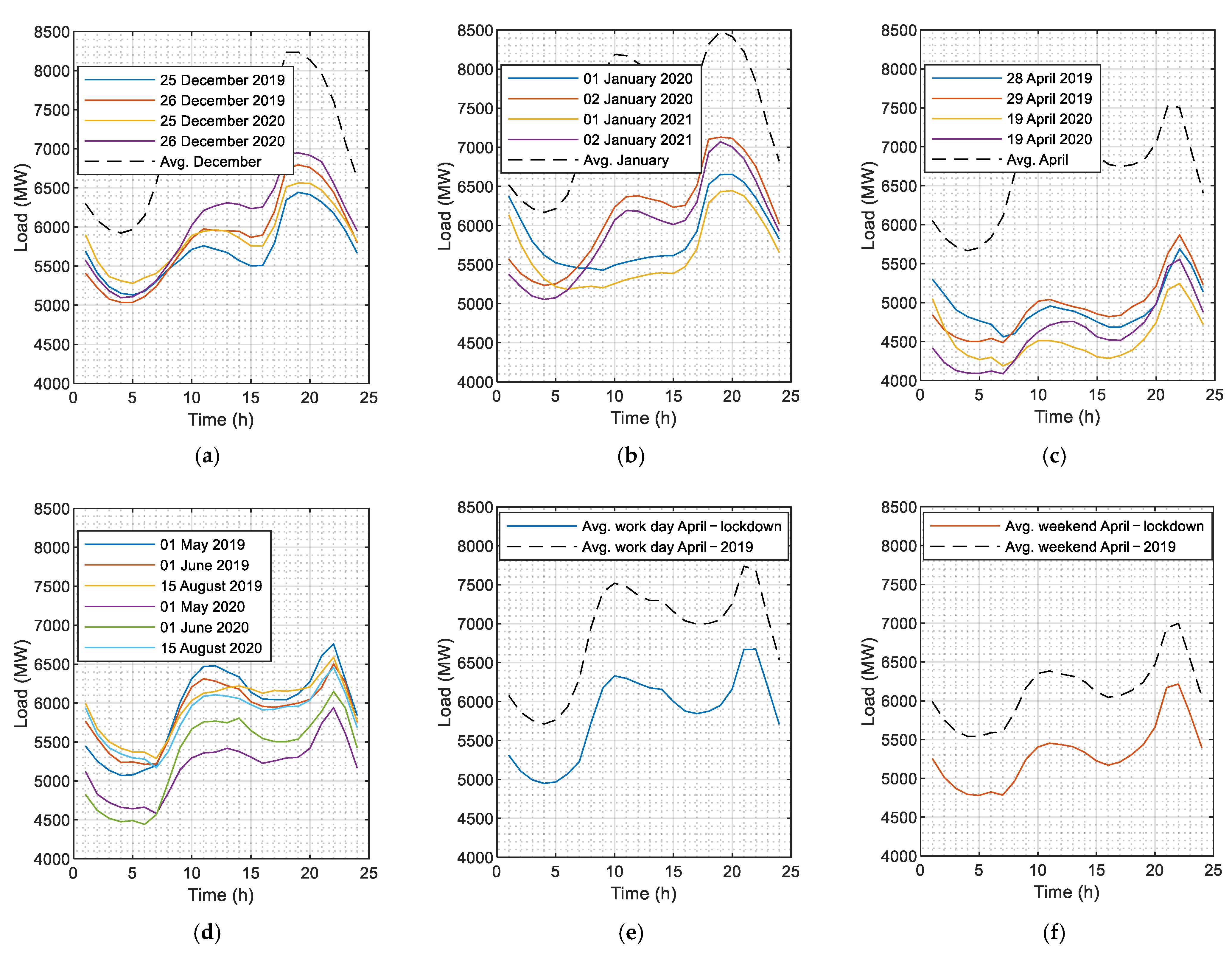
• Assessing the COVID-19 pandemic effects on the electricity demand in Romania;
• Proposing an STLF model that incorporates pandemic-related inputs, based on the previously mentioned analysis, using CNNs;
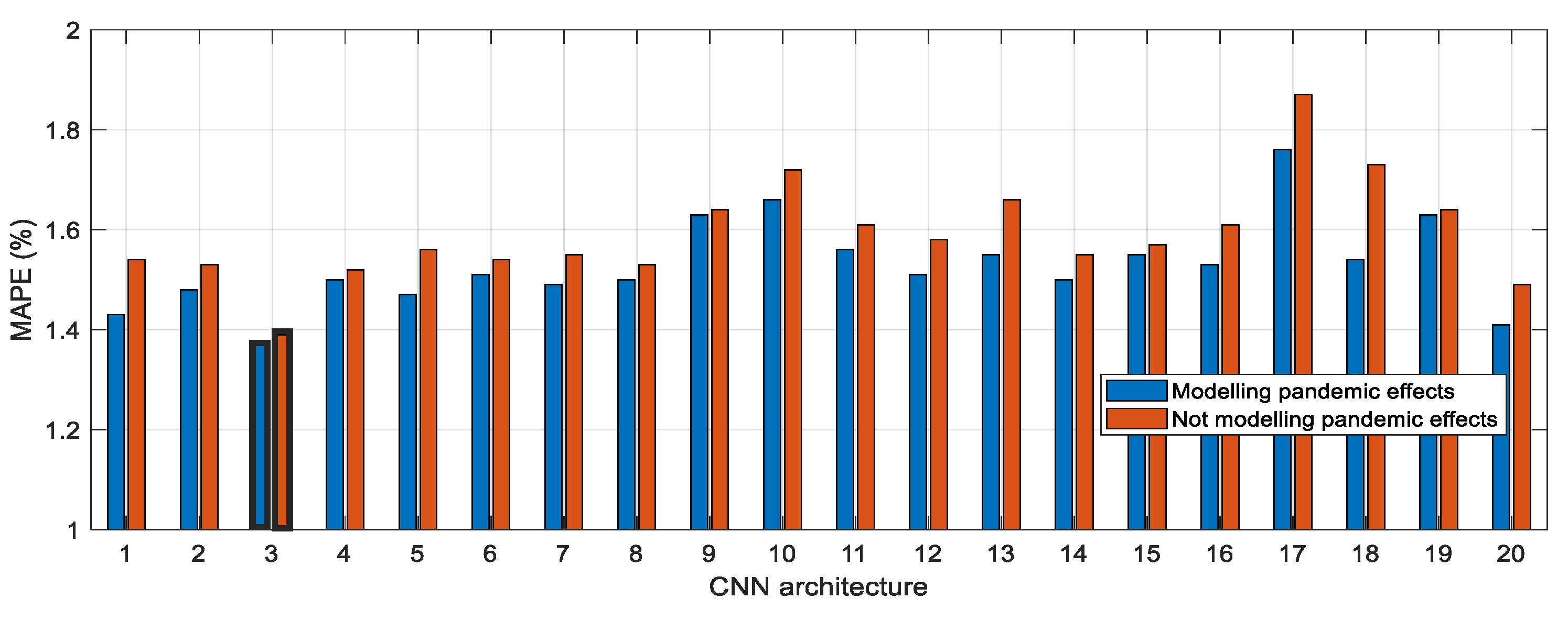
• Evaluating the benefits of including the pandemic effects in the STLF model and identifying the best CNN architecture;
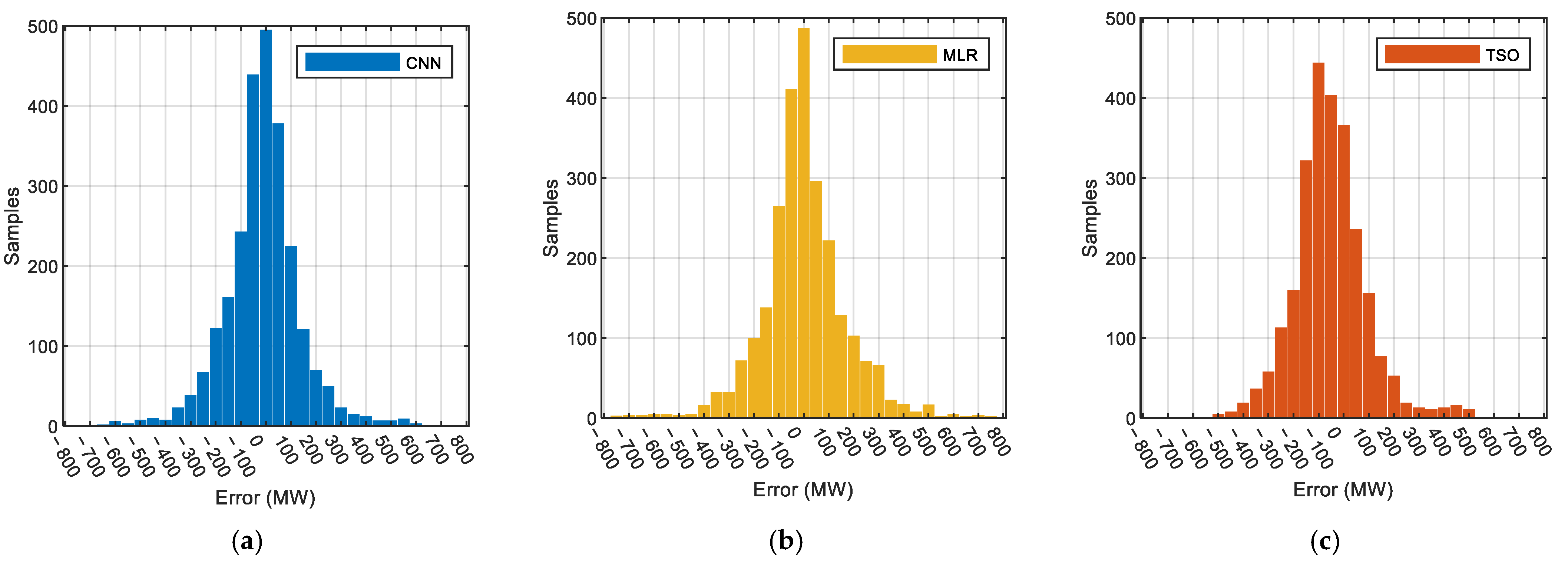
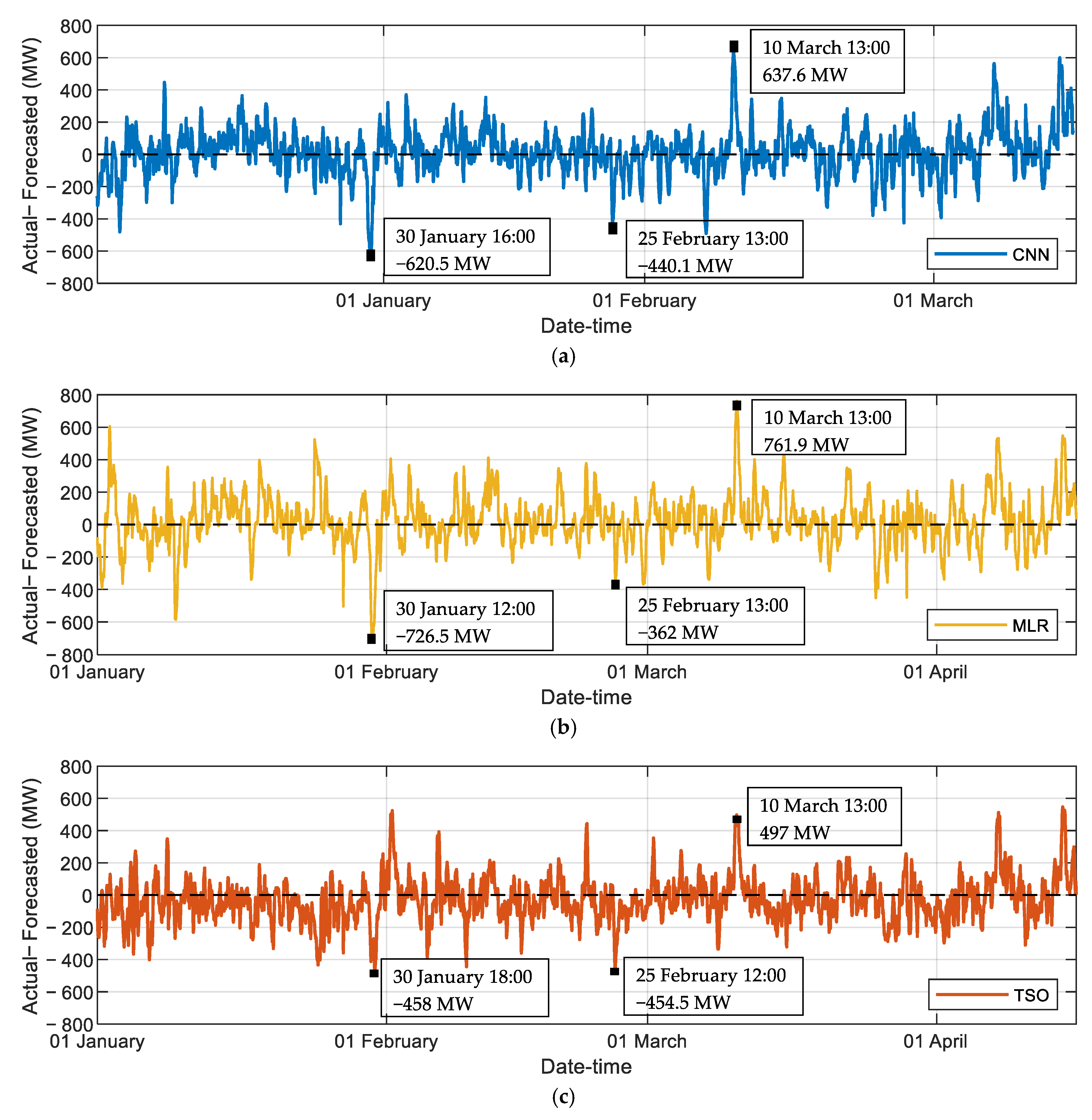
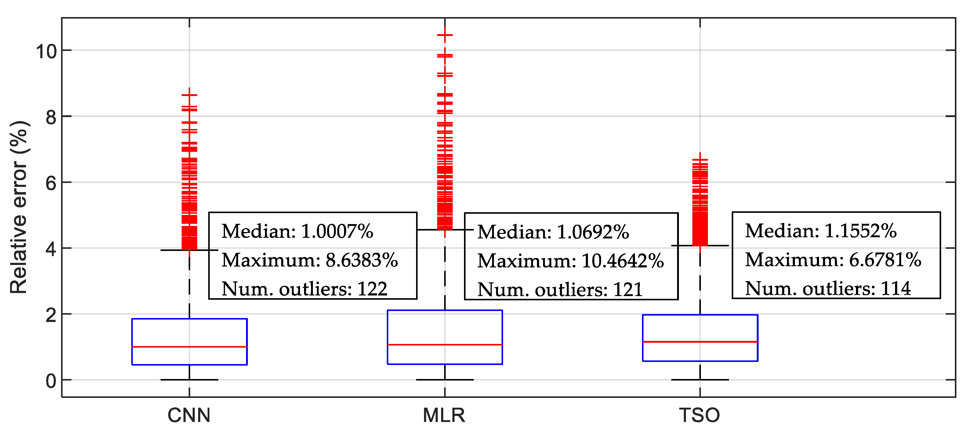
• Establishing the accuracy of the model by comparing the obtained results with two other methodologies, namely the multiple linear regression (MLR) and the results provided by the Romanian TSO.

The rest of the paper is structured as follows. Section 2 discusses the COVID-19 outbreak impact on the electricity demand in Romania. In Section 3, the implementation procedure for the load forecasting methods is described, while Section 4 exhibits the experimental results. Finally, conclusions and guidelines for future work are stated in Section 5.

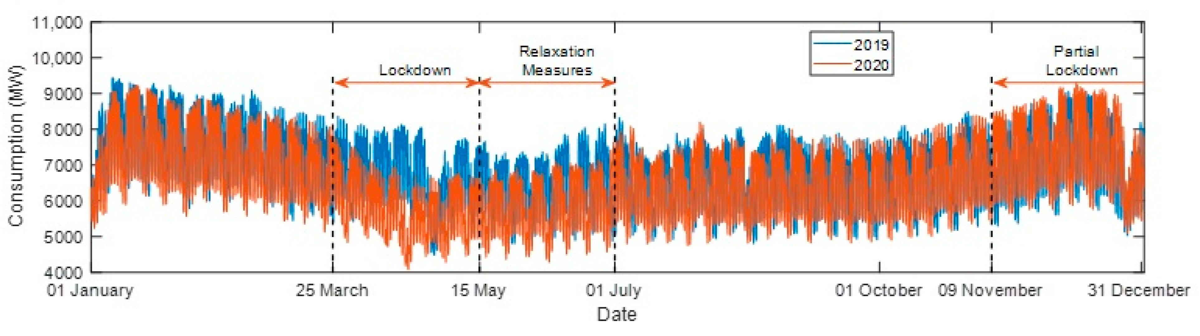
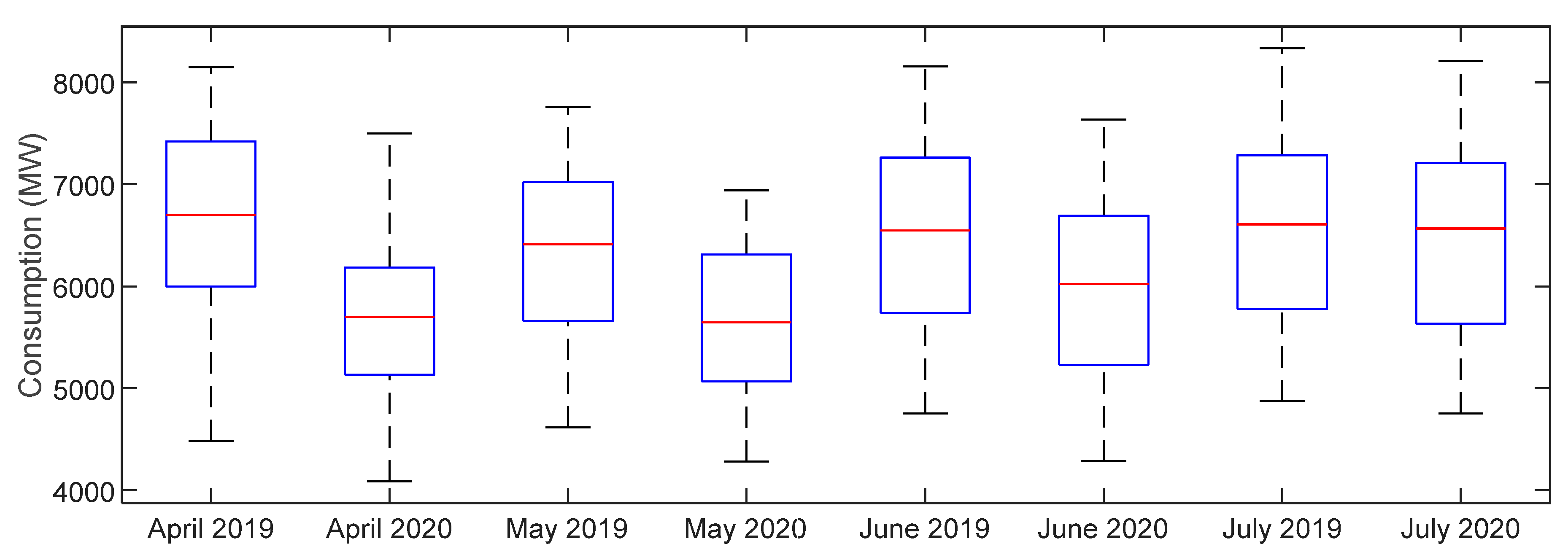
2. COVID-19 Pandemic Effects on the Electricity Demand in Romania

The first reported cases of the novel coronavirus disease were in December 2019 in the region of Hubei, China. Soon, it became clear that the disease represents a major issue; thus, the World Health Organization (WHO) declared COVID-19 to be a Public Health Emergency of International Concern on 30 January 2020 [28]. As the disease spread across the world, with several severe cases reported, in conjunction with the uncertainty regarding the effects of the virus, the WHO declared the outbreak of the novel coronavirus a global pandemic on 11 March 2020 [29]. As most countries enforced several traveling restrictions or lockdowns during COVID-19 outbreaks, the economy was greatly impacted by the pandemic.

In Romania, the first case of COVID-19 infection dated from 26 February 2020. In less than one month, on 24 March 2020, Romania reached 762 infections with the novel coronavirus. In order to reduce the spread of the disease, the government announced, through a military ordinance, national lockdown [30], allowing only essential activities, such as grocery shopping and emergency medical care. As many companies suspended their business activities, a major change in the power demand at the national level could be observed. Following the lockdown measure, the electricity consumption drastically decreased compared to the same period in previous years, as depicted in Figure 1.

Starting with the date of 15 May 2020, gradual relaxation measures were considered [31] until most restrictions were suspended on 1 July 2020. As it can be observed in Figure 1, the restrictions have a major impact on the electricity consumption in the relaxation phase as well. Following the final relaxation measures, the energy consumption restored to typical values as most economic activities recommenced. Due to the increasing number of new infections, the government imposed partial lockdown on 9 November 2020, in order to decrease the spreading rate of the disease [32], mainly consisting of a curfew within the 22.00–05.00 period.

On the first two weeks after the lockdown decision (25 March–7 April 2020), the electricity demand gradually reduced compared to the period before lockdown and to the corresponding period of 2019. For the mentioned period in 2019, the maximum load reached in the Romanian power system was 8373 MW, on 26 March. For the same period in 2020, at the beginning of the lockdown, the maximum load was 7803 MW, which was reached on 25 March, with 6.8% less than the equivalent period of the previous year. Furthermore, during the period 8 April–14 May, the peak loads in 2019 and 2020 were 8138 MW and 6958 MW, respectively, decreasing by 14.6% in 2020. Similar consequences of the lockdown were identified by the authors of [27] in the Italian power system.

To further quantify the effects of the pandemic lockdown, Figure 2 displays a boxplot representation of the monthly consumption in Romania for the most relevant months in 2019 and 2020. During the lockdown period, the consumption has been reduced significantly, as each indicator of the boxplots for the selected months of 2020 has lower value compared to its equivalent from 2019 (e.g., the median hourly consumption in April 2019 was 6676 MWh, while for April 2020, the value reduced by 14.6%, reaching only 5700 MWh). In July, after the relaxation of the measures, the consumption reached similar values compared to 2019.

In the context of the COVID-19 pandemic, demand forecasting becomes a more difficult task, as various restrictions may affect the load profile. As state-of-the-art methods for load forecasting involve neural networks trained with supervised learning, modeling of the pandemic effects represents an important feature to ensure good accuracy of new models.

3. Load Forecasting Methods

The STLF is defined as a time-series problem that requires the prediction of the next-day consumption pattern based on historical load profiles. In addition to historical values of the consumption, the electricity demand is conditioned by other numerous exogenous factors, such as weather-related data and social aspects [33]. The day-ahead load forecasting problem can be formulated by using the following equation:

$$\left[{\widehat{y}}_{t+1},\dots ,{\widehat{y}}_{t+24}\right]=f\left(y_t,y_{t-1},\dots ,y_{t-n},x_1,x_2,\dots ,x_m\right)$$

(1)

where y_i and ŷ_i are the actual load and the predicted load at time i, respectively, while x_m denotes the exogenous input m and t is the current time.

In this paper, two methodologies are investigated in solving the STLF problem, namely the classical multiple linear regression (MLR) and a convolutional neural network (CNN)-based model, the former serving as a benchmark for the CNN. Further in this section, the principles of the mentioned methods are outlined.

3.1. Multiple Linear Regression

The multiple linear regression represents a fundamental method of solving forecasting problems, employing a statistical approach. The method establishes the correlation between the predicted variable and a set of predictor variables [34].

$$y={\beta }_0+{\beta }_1{x}_1+{\beta }_2{x}_2+\dots +{\beta }_k{x}_k+\epsilon$$

(2)

where y is the predicted variable, x₁, x₂, ..., x_k are the independent variables, β₀, β₁, ..., β_k are the regression parameters, and ε is the error term.

The error term ε is considered to have the mean value of zero and constant variance; thus, the MLR model computes an estimate b of the parameters β [35].

$$\widehat{y}=b_0+b_1{x}_1+b_2{x}_2+\dots +b_k{x}_k$$

(3)

The b parameters of the MLR model are computed using the ordinary least squares method, which implies the minimization of the following equation:

$$B={\left(X^{T}X\right)}^{-1}{X}^{T}Y$$

(4)

where B, X, and Y are the matrix representations of the regression coefficients, independent variables, and the predicted variables, respectively, considering a set of n examples.

$$B=\left[\begin{array}{c}{b}_0\\ b_1\\ \begin{array}{c}⋮\\ b_k\end{array}\end{array}\right],Y=\left[\begin{array}{c}{y}_1\\ y_2\\ \begin{array}{c}⋮\\ y_n\end{array}\end{array}\right], X=\left[\begin{array}{ccc}1& x_{1,1}& \begin{array}{ccc}{x}_{1,2}& \dots & x_{1,k}\end{array}\\ 1& x_{2,1}& \begin{array}{ccc}{x}_{2,2}& \dots & x_{2,k}\end{array}\\ \begin{array}{c}⋮\\ 1\end{array}& \begin{array}{c}⋮\\ x_{n,1}\end{array}& \begin{array}{ccc}\begin{array}{c}⋮\\ x_{n,2}\end{array}& \begin{array}{c}\ddots \\ \dots \end{array}& \begin{array}{c}⋮\\ x_{n,k}\end{array}\end{array}\end{array}\right]$$

(5)

One major advantage of using statistical models, such as MLR, in load forecasting problems consists in the simplicity of the model. MLR may involve both continuous numerical values (quantitative variables) and categorical values (qualitative variables) [36] without requiring any adaptation of the model. As the regression coefficients are determined using a few matrix operations, described by Equation (4), the computation time required to solve the MLR model is significantly lower compared to other methods. Nevertheless, in load-forecasting problems, the available data are rapidly increasing, causing the MLR to be outperformed by other methods, such as neural networks. Considering its simplicity and robustness, multiple linear regression is used in this paper as a benchmark model.

The predicted variable ŷ is estimated using the input variables x and the b parameters. As the MLR method returns a single output, the multiple hour forecasting implies the computation of a corresponding set of b parameters (the B array) for each time step, which is adapted to the hourly target output Y.

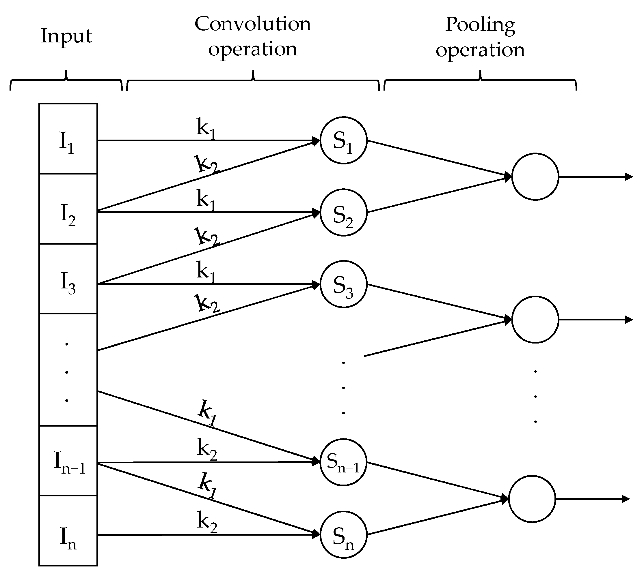
3.2. Convolutional Neural Networks (CNN)

The main feature of CNNs is the capability to extract local trends from contiguous data, which are structured in the form of an array, such as pixels in images or measured values of a time series. CNNs display state-of-the-art performance on a wide variety of applications in the image processing field, such as recognition of handwritten text [37], object detection [38], or diagnosis based on medical images [39], as well as in other fields, such as speech recognition [40] or traffic forecasting [41]. CNNs provide effective tools for solving various problems in power systems as well. In [42], a classifying model based on CNN is developed for transient stability assessment, outperforming other machine-learning methods. The authors of [43] proposed a CNN model for fault location on HVDC links. The low computational cost of CNNs allowed the authors of [44] to develop an accelerated tool for N−1 contingency evaluation.

A CNN represents a neural network that employs the convolution operation for feature extraction in at least one of its layers [45]. Considering a one-dimensional input, the convolution operation can be described by the following equation:

$$S\left(i\right)=\left(I\ast K\right)\left(i\right)={\displaystyle \sum }_{n}I\left(i+n\right)\times K\left(n\right)$$

(6)

where * represents the convolution operator, while I and K are the 1D input and the kernel, respectively. The output of the convolution operation is the feature map S.

In addition to the convolution operation, CNNs define the pooling operation, which extracts the maximum or average value of adjacent elements from a feature map, thus achieving a down-sampling of the initial feature maps. Figure 3 depicts a visual representation of the convolution and pooling operations for a one-dimensional input.

As the parameters of the kernel are multiplied with each value of the input array, a sparse connectivity of the neural network is assured, significantly reducing the number of parameters to update during training, which implies an increase in the convergence speed. Furthermore, as the kernel’s weights are shared among the elements of the input array, the neural network is able to learn and detect features regardless of the position occurred within the input [25]. Consequently, the electricity consumption patterns may be learned by a CNN and generate good results for the STLF problem. CNNs proved efficient in solving load forecasting problems using one-dimensional inputs, considering a sequence of historical consumption data as input [46]. The applications proposed in the literature involve two-dimensional CNNs as well, emphasizing the relation between the same periods from different days [47], achieving good accuracy. The model proposed in this paper is based on 1D CNN, as the model complexity is reduced compared to 2D CNNs.

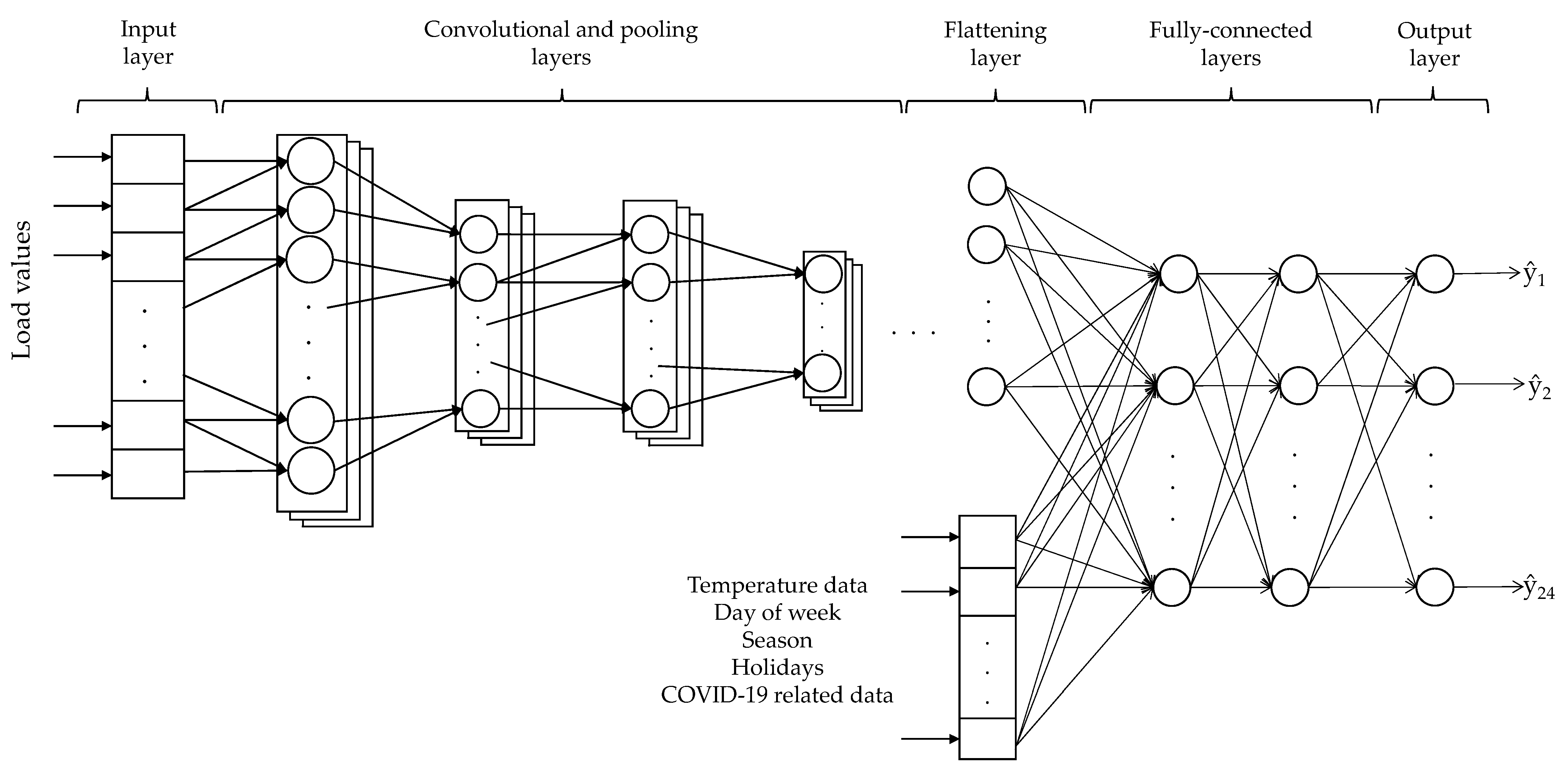
4. The Proposed Convolutional Neural Network (CNN) Model Implementation

Building on the authors’ previous work [48], the proposed load forecasting method employs several data types, including historical electricity consumption, temperature data, and social-related data derived from the calendar date, such as the day of week, season, or holiday flags. A CNN model is developed in this paper for solving the day-ahead load forecasting problem, at one-hour resolution, for the aggregated load in the Romanian power system, which considers the COVID-19 pandemic effects as well, based on the timeline of decisions taken by the government in Romania.

4.1. The Convolutional Neural Network (CNN) Structure

A typical CNN architecture is comprised of convolutional and pooling layers, as discussed in the previous section, a flattening layer, which organizes the feature maps in a one-dimensional array, and the fully connected layers, which consist of classical feed-forward neurons. The convolutional and pooling layers are designed for processing data connected spatially (e.g., pixels in an image) or temporally (e.g., load variation in time). Therefore, in the proposed model, the convolutional layer’s input is represented by the historical load values, while the exogenous data are concatenated with the neurons in the flattening layer and forwarded to the fully connected layers, as depicted in Figure 4. The parameters of the neural network are discussed in Section 5.

The activation function used for each convolutional and fully connected layer is the exponential linear unit (ELU), as it outperforms the rectified linear unit (ReLU) and its variations [49]. The output of ELU function is computed as follows:

$$y=\{\begin{array}{c}x x>0\\ \alpha \left(e^x-1\right) x\le 0 \end{array}$$

(7)

where x and y are the neuron’s input and output, respectively. The hyperparameter α is set to 1 in this study.

For capturing complex features of the load profile, the consumption values from the previous week, consisting of 168 hourly loads, are used as input for the convolutional layer. The exogenous variables employed in the proposed model consist of temperature, date-related, and COVID-19 pandemic data. For temperatures, values for the past week are used, as well as the forecast for the day ahead, as meteorological forecasts can be considered accurate. The calendar date reveals important features for an STLF model, as the load is affected by various social factors (e.g., working day or weekend). In this regard, categorical variables, which may only accept values of 0 and 1, are created to specify the day of week, season, and whether the day is a holiday, using the one-hot coding technique [50].

Figure 5 depicts the electricity consumption during various holidays, such as Christmas or New Years, and during the lockdown from 2020. As it can be observed, the load profiles have specific shapes during the most important holidays (i.e., Christmas, New Years, and Easter); thus, using a single categorical input for all holidays is insufficient. Therefore, three more categorical variables are created in order to indicate the occurrence of the three mentioned holidays.

As the measures for diminishing the COVID-19 infection rate affected the economic activity and thus the electricity consumption, neural network-based forecasting methods should be designed to contain pandemic-related data. The proposed STLF model includes the pandemic effects through categorical variables, by indicating if any restrictions are applied for the forecasted day. These restrictions are known based on governmental decisions, which are publicly announced. As depicted in Figure 1, three major periods could be identified so far in Romania (i.e., the national lockdown, a period of gradual relaxation, and the partial lockdown). In this regard, a categorical variable is defined for each of the three major sets of restrictions, specifying the measures applied for each day in the dataset. The periods discussed in Section 2 are described in

Table 1. Pandemics conditions in Romania.

Pandemic Restrictions Period	Starting Date	Ending Date
National lockdown	25 March 2020	15 May 2020
Gradual relaxation	16 May 2020	1 July 2020
Partial lockdown	9 November 2020	15 April 2021

. Similar to the temperature inputs, the holiday effect and pandemic data for the past 7 days and for the forecasted day are introduced in the model.

As depicted in Figure 4, the output of the model consists in the load forecast for the next 24 h. To summarize the input variables of the proposed model,

Table 2. Input variables of the proposed model.

Variable Type	Type of Data	Temporal Characteristics	One Hot Encoding
Load	Hourly values	Past 168 h	No
Temperature	Min./avg./max. daily values	Past 7 days and forecasted day	No
Day of Week	Monday/Tuesday/Wednesday/Thursday/Friday/Saturday/Sunday	Forecasted day	Yes
Season	Spring/Summer/Autumn/Winter	Forecasted day	Yes
Holidays	No holiday/Typical holiday/Christmas/New Year’s Day/Easter	Past 7 days and the forecasted day	Yes
Pandemic restrictions	No restrictions/lockdown/gradual relaxation/partial lockdown	Past 7 days and the forecasted day	Yes

presents the variable types and their implementation characteristics.

4.2. Convolutional Neural Network (CNN) Training and Performance Evaluation

Introduced in [51], the Nesterov-accelerated Adaptive Moment Estimation (Nadam) optimizer combines the nesterov momentum and the Adam algorithm. The performance achieved by Nadam in training convolutional neural networks exceeds other optimizers, such as stochastic gradient descent (SGD), adaptive gradient (AdaGrad), or the standard Adam [52]. In this regard, the proposed method employs the Nadam optimizer in training the model. The considered loss function for the CNN model is represented by the Mean Squared Error (MSE) computed with Equation (8), where y and ŷ define the actual load and predicted load, and n is the number of samples.

$$MSE=\frac{1}{n}{\displaystyle \sum }_1^n{\left(y-\widehat{y}\right)}^2$$

(8)

A major challenge in training neural networks models is represented by the occurrence of overfitting, which consists in achieving good accuracy for the training dataset yet performing poorly for the testing dataset. To improve generalization, thus reducing overfitting, several techniques may be employed, such as early stopping, dropout, and L₁ or L₂ regularization [53]. In this paper, an early stopping criterion is implemented, which consists of monitoring the value of the loss function for the validation set during training and stopping the training process if the performance on the validation set does not improve over 1000 epochs. Additionally, the L₁ and L₂ regularization techniques are applied in the developed CNN model to further avoid overfitting. These regularization methods introduce supplemental terms to the loss function as follows:

$$E\left(w\right)=E_0\left(w\right)+{\lambda }_1{\displaystyle \sum }_i\left|w_i\right|+\frac{1}{2}{\lambda }_2{\displaystyle \sum }_i{w}_i^2$$

(9)

where E₀(w) represents the initial loss function, which was computed using Equation (8), w are the weights of the neural network, and λ₁ and λ₂ are the regularization coefficients.

The L₁ regularization method aims at minimizing the neural network’s weights with respect to the λ₁ coefficient, representing a feature selection mechanism. As the input of the proposed model consists of a significant number of categorical variables, leading to a degree of sparsity in the data, the L₁ regularization may reduce the value of weights associated with insignificant features [54]. Described by the sum of squared weights, the L₂ regularization technique prevents overfitting of data during training by hindering the weights from reaching high values if it is not necessary [55]. In this paper, the considered values for the regularization coefficients are 1 for λ₁ and 0.1 for λ₂, respectively.

The evaluation of the model’s accuracy is performed by using several metrics widely applied in the literature [56,57,58]. Additionally, to the MSE index, which is previously defined, the Mean Absolute Error (MAE), the Mean Absolute Percentage Error (MAPE), and the Root Mean Square Error (RMSE) were used as well.

$$\mathrm{MAE}=\frac{1}{n}{\displaystyle \sum }_1^n\left|y-\widehat{y}\right|$$

(10)

$$\mathrm{MAPE}=\frac{1}{n}{\displaystyle \sum }_1^n\left|\frac{y-\widehat{y}}{y}\right|100$$

(11)

$$\mathrm{RMSE}=\sqrt{\frac{1}{n}{\displaystyle \sum }_1^n{\left(y-\widehat{y}\right)}^2}$$

(12)

For the CNN model implementation, Keras, a machine learning library built in Python, was employed using TensorFlow as the backend. Regarding the MLR method, the scikit-learn machine learning library is used to define the model. The neural network training was performed on a personal computer with NVIDIA GPU GeForce GTX 1050 Ti. As TensorFlow applies GPU parallel computing techniques in the training process of neural networks, the time is substantially reduced compared to the standard CPU computing [59]. Therefore, the possibility of studying various architectures is facilitated.

5. Simulation Results

5.1. Dataset Description

The proposed CNN model is trained in this case study using data collected over the period 16 November 2012—15 April 2021, aiming at forecasting the day-ahead aggregated load for the Romanian power system. According to the model description presented in the previous section, the proposed STLF methodology requires previous values of the electricity consumption, temperature data, date-related information, and COVID-19 pandemic data. The historical load in the Romanian power system with hourly resolution is available at the Romanian TSO website [60]. For modeling the temperature effect, the minimum, maximum, and average daily values measured in Bucharest city were collected from the wunderground web service [61]. As discussed in previous sections, the pandemic impact is modeled considering the governmental decisions in Romania.

5.2. Convolutional Neural Network (CNN) Parameter Tuning

Achieving good performances with neural network-based models heavily relies on the proper design of the architecture. As neural networks consist of numerous parameters and hyperparameters that may affect the accuracy of the model, identifying the optimal architecture represents a difficult task, considering the amount of time required to train complex models. The influence of the convolutional layers’ parameters (i.e., the number of convolutional layers, number of filters used, and their dimension) on the model performance is further studied. In this regard, 20 different CNN architectures are proposed, having the number of convolutional layers varied from one up to three. Furthermore, the effect of pooling layers is analyzed.

Table 3. Description of the considered Convolutional Neural Network (CNN) architectures.

Architecture	Convolutional Layers	(Number of Convolutional Filters/Filter Size)	Pooling Filter Size	Dense Layers Size
1	1	(15/5)	-	(24,24)
2		(15/5)	2
3		(15/3)	-
4		(15/3)	2
5		(15/9)	-
6		(15/9)	2
7	2	((15/3), (15/9))	-
8		((15/3), (15/9))	(2,2)
9		((5/3), (1/9))	-
10		((5/3), (1/9))	(2,2)
11		((15/7), (15/5))	-
12		((15/7), (15/5))	(2,2)
13		((5/13), (1/3))	-
14		((5/13), (1/3))	(2,2)
15		((5/7), (1/5))	-
16		((5/7), (1/5))	(2,2)
17	3	((15/9), (15/5), (15/3))	-
18		((15/9), (15/5), (15/3))	(2,2,2)
19		((5/13), (5/9), (1/5))	-
20		((5/13), (5/9), (1/5))	(2,2,2)

summarizes the particularities of each considered architecture.

The available dataset is split among the training, validation, and testing phases, as follows:

• The days of 2021 (1 January–15 April) are used for testing the accuracy of the neural network;
• 70% of the remaining data are used for training;
• 30% of the remaining data are used for validation.

The precision assessment is conducted for each of the 20 previously defined architectures, by computing the MAE, MAPE, MSE, and RMSE values for the testing dataset. The results achieved by the considered architectures are presented in

Table 4. Convolutional Neural Network (CNN) model performance for various architectures.

		Modeling Pandemic Effects				Not Modeling Pandemic Effects
		MAE	MAPE	MSE	RMSE	MAE	MAPE	MSE	RMSE
CNN Architecture	1	108.09	1.43	23.475	153.2	117.3	1.54	28.157	167.8
	2	111.6	1.48	24.868	157.7	116	1.53	30.222	173.8
	3	104	1.37	20.841	144.36	105.9	1.39	23.059	151.9
	4	112.5	1.50	25.852	160.8	115.9	1.52	27.783	166.7
	5	111.1	1.47	24.946	157.9	119.6	1.56	29.084	170.5
	6	114	1.51	27.043	164.5	116.9	1.54	29.211	170.9
	7	113.3	1.49	26.591	163	118	1.55	29.798	172.6
	8	114.3	1.5	26.919	164	117.5	1.53	28.523	168.9
	9	123	1.63	26.513	162.8	124.3	1.64	31.649	177.9
	10	124.9	1.66	29.317	171.2	130.7	1.72	33.081	181.9
	11	118.9	1.56	29.637	172.2	122.1	1.61	32.019	178.9
	12	114.9	1.51	26.849	163.9	120.7	1.58	29.996	173.2
	13	117.2	1.55	26.669	163.3	125.7	1.66	32.297	179.7
	14	113.8	1.50	23.611	153.7	117.7	1.55	27.263	165.1
	15	117.4	1.55	26.694	163.4	119.6	1.57	27.157	164.8
	16	114.7	1.53	24.657	157	122.5	1.61	28.472	168.7
	17	133.3	1.76	36.118	190	141.5	1.87	43.499	208.6
	18	118.2	1.54	28.558	169	131.4	1.73	35.548	188.5
	19	125.9	1.63	31.722	178.1	124.3	1.64	31.029	176.2
	20	107.2	1.41	21.221	145.7	112.2	1.49	23.090	152

Mean Absolute Error (MAE), Mean Absolute Percentage Error (MAPE), Root Mean Square Error (RMSE).

. Furthermore, in order to evaluate the importance of considering pandemic effects, the neural network is also trained without including the pandemic impact.

As it can be observed in Table 4, the best performance by means of all evaluation metrics is achieved by architecture 3, when the pandemic effects are included in the model, reaching an MAPE value of only 1.37%. Overall, better results are achieved with less convolutional layers, as using three convolutional layers led to poor performances due to overfitting (e.g., for architectures 17 and 19, the MAPE values are 1.76% and 1.63%, respectively). Applying the pooling operation generates worse results for the architectures with one convolutional layer, while it improves the performance for architectures with three layers. When two layers are used, the pooling operation improves the accuracy of the model in the majority of the cases, with few exceptions, namely architectures 7–10, where using pooling layers lead to marginally worse results. Therefore, for more convolutional layers used, the pooling layers can improve the model’s accuracy by downsizing the input volume to extract the most important information, as the model is prone to overfit. However, the down-sampling through pooling may lose relevant information when using one convolutional layer, leading to worsen accuracy.

To better emphasize the impact of including pandemic effects data in the model, Figure 6 depicts the values of MAPE for the 20 proposed architectures when the pandemic conditions are acknowledged against the results obtained without considering pandemic data. During the testing days (from 1 January to 15 April 2021), partial lockdown restrictions were applied at the national level in Romania. As Figure 6 reveals, a better accuracy is attained for each analyzed architecture when pandemic effects are included in the model, achieving an average reduction of the errors by 4.3%. Therefore, considering pandemic-related input data in the model improves the performance of the CNN model for the testing set.

5.3. The Proposed Model Performance Evaluation

In order to benchmark the proposed CNN model, a comparative analysis is conducted between the best CNN architecture identified in the previous section, a standard MLR model, and the consumption values estimated by the Romanian TSO, Transelectrica. For equity between the models, the same input data used to train the CNN were considered in the MLR model. The day-ahead load forecast results of the TSO are publicly accessible on the official web page [62].

Firstly,

Table 5. Performance evaluation for Convolutional Neural Network (CNN), Multiple Linear Regression (MLR), and Transmission System Operator (TSO).

	MAE	MAPE	MSE	RMSE
CNN	104	1.37	20841	144.36
MLR	116.7	1.54	26965	164.2
TSO	108.15	1.45	20464	143.05

presents the values of evaluation metrics achieved by each method for the considered testing period. The proposed model achieved the best results in terms of MAE and MAPE, while the TSO shows marginally better values for MSE and RMSE. The linear regression method exhibits the lowest performances among the three sets of results.

To better comprehend the performance of the proposed model, a more detailed analysis of the forecasting results is further conducted for the three considered methodologies. Figure 7 depicts the distribution of absolute errors for the testing set, which are determined as the difference of the actual and forecasted values of the consumption.

The proposed CNN model displays a zero-centered distribution of errors, with 37% of the samples laying in the (−50:50) MW range, thus resulting in good values for the evaluation metrics. However, the reached error for few samples exceeds 500 MW. Conversely, for the TSO results, a skewed distribution can be observed, which is centered around the −100 MW mark, attaining only 30% of the errors in the interval (−50:50) MW. The distribution of errors produced by the TSO results is narrower compared to that of the CNN, as the error of each sample is contained in the interval (−500:500) MW. To identify the days when high forecasting errors occurred, Figure 8 depicts the difference between the actual and the forecasted values sequentially for the testing period.

For several days (e.g., 30 January, 25 February, and 10 March), which exhibited atypical behavior of the load, each of the analyzed methodologies presented high values of the errors, as depicted in Figure 8. During special days, namely 1 January and 2 January, CNN and TSO achieved good accuracy, with the maximum errors being 318 MW and 317 MW, respectively. On the other hand, MLR displayed poor performances on the mentioned days, indicating that the model is not able to extract the relevant features regarding the holiday effects on the load profile.

The proposed CNN model’s accuracy is further evaluated by comparing the relative errors for the CNN, MLR, and TSO, employing the boxplot representation from Figure 9.

The CNN model was the most consistent in achieving precise forecasts, as the median value of the errors was 1%, with 0.155% better compared to the TSO results. As previously revealed, high errors are occurring in several atypical days, as the maximum relative error for the CNN reached 8.64%, while the maximum error for the TSO is 6.68%.

6. Conclusions

The COVID-19 pandemic raises major concerns for public health and for the economic field as well. As a consequence of the new socioeconomic conditions, the electricity demand is drastically affected by the changes in the economic sectors. In this paper, a CNN model was implemented to solve the STLF for the aggregated load in the Romanian power system, which incorporates conventional exogenous factors (weather, day of the week, season, etc.) and the pandemic effects as well. Modeling the COVID-19 pandemic restrictions represents an important feature of novel load forecasting methods, as governmental decisions and the rate of infection influence the economic activity, thus changing the electricity demand at both aggregated and individual consumption levels. Regardless of the future conditions and state of the pandemic, its impact should be further acknowledged, as COVID-19 triggered important disruptions and reforms in many areas of activities (e.g., work from home and online education). These data must be considered, since load forecasting models based on machine learning techniques require information from the past to learn. Otherwise, if lockdown periods, or other major events regarding the pandemic, are not properly flagged, a decrease in accuracy occurs due to the lack of these biasing data.

Frequently used metrics, namely the MAE, MAPE, MSE, and RMSE, were used in this study in order to identify the most performant CNN model design. An analysis on the importance of considering pandemic effects was further conducted by training the studied architectures, firstly by including the pandemic-related inputs and subsequently by disregarding them. The results showed a reduction of the errors for all the assessed architectures when the COVID-19 restrictions are considered, proving the necessity of inserting these socioeconomic aspects in the model. Furthermore, the proposed model’s performance was compared with the results obtained by a multiple linear regression model and the results acquired from the Romanian TSO. The CNN model presents promising results, as it was the most consistent method in obtaining reduced forecasting errors for the analyzed testing period.

Future work focuses on load and generation forecasting at lower aggregation levels for optimal day-ahead scheduling of microgrids, considering electricity market participation as well. As deep neural networks require a large amount of data to provide good results, data augmentation techniques will be investigated in the future, to enlarge the training dataset based on available inputs.

References

1. Dec, G.; Drałus, G.; Mazur, D.; Kwiatkowski, B. Forecasting Models of Daily Energy Generation by PV Panels Using Fuzzy Logic. Energies 2021, 14, 1676. [Google Scholar] [CrossRef]
2. Wang, H.; Lei, Z.; Zhang, X.; Zhou, B.; Peng, J. A review of deep learning for renewable energy forecasting. Energy Convers. Manag. 2019, 198, 111799. [Google Scholar] [CrossRef]
3. Țiboacă, M.; Costinaș, S.; Rădan, P. Design of Short-Term Wind Production Forecasting Model using Machine Learning Algorithms. In Proceedings of the 2021 12th International Symposium on Advanced Topics in Electrical Engineering (ATEE), Bucharest, Romania, 25–27 March 2021; Institute of Electrical and Electronics Engineers: Piscataway, NJ, USA, 2021. [Google Scholar] [CrossRef]
4. Hong, T.; Fan, S. Probabilistic electric load forecasting: A tutorial review. Int. J. Forecast. 2016, 32, 914–938. [Google Scholar] [CrossRef]
5. Luo, J.; Hong, T.; Yue, M. Real-time anomaly detection for very short-term load forecasting. J. Mod. Power Syst. Clean Energy 2018, 6, 235–243. [Google Scholar] [CrossRef] [Green Version]
6. Chen, K.; Chen, K.; Wang, Q.; He, Z.; Hu, J.; He, J. Short-Term Load Forecasting With Deep Residual Networks. IEEE Trans. Smart Grid 2019, 10, 3943–3952. [Google Scholar] [CrossRef] [Green Version]
7. Dong, X.; Qian, L.; Huang, L. A CNN based bagging learning approach to short-term load forecasting in smart grid. In Proceedings of the 2017 IEEE SmartWorld, Ubiquitous Intelligence & Computing, Advanced & Trusted Computed, Scalable Computing & Communications, Cloud & Big Data Computing, Internet of People and Smart City Innovation (SmartWorld/SCALCOM/UIC/ATC/CBDCom/IOP/SCI), San Francisco, CA, USA, 4–8 August 2017. [Google Scholar]
8. Juberias, G.; Yunta, R.; Garcia Moreno, J.; Mendivil, C. A new ARIMA model for hourly load forecasting. In Proceedings of the 1999 IEEE Transmission and Distribution Conference (Cat. No. 99CH36333), New Orleans, LA, USA, 11–16 April 1999. [Google Scholar]
9. Bercu, S.; Proïa, F. A SARIMAX coupled modelling applied to individual load curves intraday forecasting. J. Appl. Stat. 2013, 40, 1333–1348. [Google Scholar] [CrossRef] [Green Version]
10. Li, W.; Han, Z.-H.; Niu, D.-X. Improved genetic algorithm-GM(1,1) for power load forecasting problem. In Proceedings of the 2008 Third International Conference on Electric Utility Deregulation and Restructuring and Power Technologies, Nanjing, China, 6–9 April 2008. [Google Scholar]
11. Ghanbari, A.; Abbasian-Naghneh, S.; Hadavandi, E.; Ghanbari, A. An intelligent load forecasting expert system by integration of ant colony optimization, genetic algorithms and fuzzy logic. In Proceedings of the 2011 IEEE Symposium on Computational Intelligence and Data Mining (CIDM), Paris, France, 11–15 April 2011. [Google Scholar]
12. Bucolo, M.; Fortuna, L.; Nelke, M.; Rizzo, A.; Sciacca, T. Prediction models for the corrosion phenomena in Pulp & Paper plant. Control Eng. Pract. 2002, 10, 227–237. [Google Scholar]
13. Cevik, H.H.; Çunkaş, M. Short-term load forecasting using fuzzy logic and ANFIS. Neural Comput. Appl. 2015, 26, 1355–1367. [Google Scholar] [CrossRef]
14. Zhou, S.-M.; Gan, J.Q. Low-level interpretability and high-level interpretability: A unified view of data-driven interpretable fuzzy system modelling. Fuzzy Sets Syst. 2008, 159, 3091–3131. [Google Scholar] [CrossRef]
15. Metaxiotis, K.; Kagiannas, A.; Askounis, D.; Psarras, J. Artificial intelligence in short term electric load forecasting: A state-of-the-art survey for the researcher. Energy Convers. Manag. 2003, 44, 1524–1534. [Google Scholar] [CrossRef]
16. Ceperic, E.; Ceperic, V.; Baric, A. A Strategy for Short-Term Load Forecasting by Support Vector Regression Machines. IEEE Trans. Power Syst. 2013, 11, 4356–4364. [Google Scholar] [CrossRef]
17. Hernández, L.; Baladrón, C.; Aguiar, J.M.; Carro, B.; Sánchez-Esquevilas, A.; Lloret, J. Artificial neural networks for short-term load forecasting in microgrids environment. Energy 2014, 75, 252–264. [Google Scholar] [CrossRef]
18. Tang, X.; Dai, Y.; Wang, T. Short-term power load forecasting based on multi-layer bidirectional recurrent neural network. IET Gener. Transm. Distrib. 2019, 13, 3847–3854. [Google Scholar] [CrossRef]
19. Ke, K.; Hongbin, S.; Chengkang, Z.; Brown, C. Short-term electrical load forecasting method based on stacked auto-encoding and GRU neural network. Evol. Intell. 2019, 12, 385–394. [Google Scholar] [CrossRef]
20. Hossain, M.S.; Mahmood, H. Short-Term Load Forecasting Using an LSTM Neural Network. In Proceedings of the IEEE Power and Energy Conference at Illinois (PECI), Champaign, IL, USA, 27–28 February 2020. [Google Scholar]
21. Bouktif, S.; Fiaz, A.; Ouni, A.; Serhani, M.A. Single and Multi-Sequence Deep Learning Models for Short and Medium Term Electric Load Forecasting. Energies 2019, 12, 149. [Google Scholar] [CrossRef] [Green Version]
22. Sidorov, D.; Tao, Q.; Muftahov, I.; Zhukov, A.; Karamov, D.; Dreglea, A.; Liu, F. Energy balancing using charge/discharge storages control and load forecasts in a renewable-energy-based grids. In Proceedings of the 38th Chinese Control Conference, Guangzhou, China, 27–30 July 2019; pp. 6865–6870. [Google Scholar]
23. Khan, S.; Javaid, N.; Chand, A.; Khan, A.B.M.; Rashid, F.; Afridi, I.U. Electricity Load Forecasting for Each Day of Week Using Deep CNN. In Proceedings of the International Conference on Advanced Information Networking and Applications, Matsue, Japan, 27–29 March 2019; Volume 927, pp. 1107–1119. [Google Scholar]
24. Kuo, P.-H.; Huang, C.-J. A High Precision Artificial Neural Networks Model for Short-Term Energy Load Forecasting. Energies 2018, 11, 213. [Google Scholar] [CrossRef] [Green Version]
25. Goodfellow, I.J.; Bengio, Y.; Courville, A. Deep Learning; MIT Press: Cambridge, MA, USA, 2016. [Google Scholar]
26. Navon, A.; Machlev, R.; Carmon, D.; Onile, A.E.; Belikov, J.; Levron, Y. Effects of the COVID-19 Pandemic on Energy Systems and Electric Power Grids—A Review of the Challenges Ahead. Energies 2021, 14, 1056. [Google Scholar] [CrossRef]
27. Ghiani, E.; Galici, M.; Mureddu, M.; Pilo, F. Impact on Electricity Consumption and Market Pricing of Energy and Ancillary Services during Pandemic of COVID-19 in Italy. Energies 2020, 13, 3357. [Google Scholar] [CrossRef]
28. World Health Organization. Available online: https://www.who.int/news/item/30-01-2020-statement-on-the-second-meetingof-the-international-health-regulations-(2005)-emergency-committee-regarding-the-outbreak-of-novel-coronavirus-(2019-ncov) (accessed on 10 May 2021).
29. Cucinotta, D.; Vanelli, M. WHO declares COVID-19 a pandemic. Acta Bio Med. Atenei Parm. 2020, 91, 157–160. [Google Scholar]
30. Ministery of Internal Affairs. Military Ordinance no. 3 of 24 March 2020. Available online: https://www.mai.gov.ro/ordonanta-militara-nr-3-din-24-03-2020-privind-masuri-de-prevenire-a-raspandirii-covid-19/ (accessed on 10 May 2021).
31. Ministery of Internal Affairs. Decision no. 24/2020 from 14 May 2020. Available online: https://www.mai.gov.ro/hotarare-nr-24-din-14-05-2020-privind-aprobarea-instituirii-starii-de-alerta-la-nivel-national-si-a-masurilor-de-prevenire-si-control-a-infectiilor-in-contextul-situatiei-epidemiologice-generate/ (accessed on 10 May 2021).
32. Romanian Government. Available online: https://gov.ro/en/ (accessed on 10 May 2021).
33. Nichiforov, C.; Stamatescu, G.; Stamatescu, I.; Făgărăşan, I.; Iliescu, S.S. Building Electrical Load Forecasting through Neural Network Models with Exogenous Inputs. In Proceedings of the 23rd International Conference on System Theory, Control and Computing (ICSTCC), Sinaia, Romania, 9–11 October 2019. [Google Scholar]
34. Olive, D. Linear Regression; Springer International Publishing: Cham, Switzerland, 2017. [Google Scholar]
35. Amral, N.; Ozveren, C.S.; King, D. Short term load forecasting using Multiple Linear Regression. In Proceedings of the 2007 42nd International Universities Power Engineering Conference, Brighton, UK, 4–6 September 2007. [Google Scholar]
36. Hong, T.; Wang, P.; Willis, H.L. A naïve multiple linear regression benchmark for short term load forecasting. In Proceedings of the Power and Energy Society General Meeting, Detroit, MI, USA, 24–29 July 2011. [Google Scholar]
37. LeCun, Y.; Kavukcuoglu, K.; Farabet, C. Convolutional networks and applications in vision. In Proceedings of the 2010 IEEE International Symposium, Circuits and Systems (ISCAS), Paris, France, 30 May–2 June 2010; Volume 201, pp. 253–256. [Google Scholar]
38. Erhan, D.; Szegedy, C.; Toshev, A.; Anguelov, D. Scalable Object Detection Using Deep Neural Networks. In Proceedings of the IEEE Conference on Computer Vision and Pattern Recognition, Columbus, OH, USA, 24–27 June 2014; pp. 2147–2154. [Google Scholar]
39. Ting, F.F.; Tan, Y.J.; Sim, K.S. Convolutional neural network improvement for breast cancer classification. Expert Syst. Appl. 2019, 120, 103–115. [Google Scholar] [CrossRef]
40. Qian, Y.; Bi, M.; Tan, T.; Yu, K. Very Deep Convolutional Neural Networks for Noise Robust Speech Recognition. IEEE/ACM Trans. Audio Speech Lang. Process. 2016, 24, 2263–2276. [Google Scholar] [CrossRef]
41. Ma, Y.; Zhang, Z.; Ihler, A. Multi-Lane Short-Term Traffic Forecasting With Convolutional LSTM Network. IEEE Access 2020, 8, 34629–34643. [Google Scholar] [CrossRef]
42. Shi, Z.; Yao, W.; Zeng, L.; Wen, J.; Fang, J.; Ai, X.; Wen, J. Convolutional neural network-based power system transient stability assessment and instability mode prediction. Appl. Energy 2020, 263, 114586. [Google Scholar] [CrossRef]
43. Lan, S.; Chen, M.-J.; Chen, D.-Y. A novel HVDC double-terminal non-synchronous fault location method based on convolutional neural network. IEEE Trans. Power Deliv. 2019, 34, 848–857. [Google Scholar] [CrossRef]
44. Du, Y.; Li, F.; Li, J.; Zheng, T. Achieving 100x acceleration for N-1 contingency screening with uncertain scenarios using deep convolutional neural network. IEEE Trans. Power Syst. 2019, 34, 3303–3305. [Google Scholar] [CrossRef]
45. Aggarwal, C. Neural Networks and Deep Learning: A Textbook; Springer: Cham, Switzerland, 2018. [Google Scholar]
46. Pramono, S.H.; Rohmatillah, M.; Maulana, E.; Hasanah, R.N.; Hario, F. Deep Learning-Based Short-Term Load Forecasting for Supporting Demand Response Program in Hybrid Energy System. Energies 2019, 12, 3359. [Google Scholar] [CrossRef] [Green Version]
47. Shen, Y.; Ma, Y.; Deng, S.; Huang, C.-J.; Kuo, P.-H. An Ensemble Model based on Deep Learning and Data Preprocessing for Short-Term Electrical Load Forecasting. Sustainability 2021, 13, 1694. [Google Scholar] [CrossRef]
48. Tudose, A.; Sidea, D.; Picioroaga, I.; Boicea, V.; Bulac, C. A CNN Based Model for Short-Term Load Forecasting: A Real Case Study on the Romanian Power System. In Proceedings of the 2020 55th International Universities Power Engineering Conference (UPEC), Turin, Italy, 1–4 September 2020. [Google Scholar]
49. Clevert, D.; Unterthiner, T.; Hochreiter, S. Fast and Accurate Deep Network Learning by Exponential Linear Units (ELUs). In Proceedings of the 4th International Conference on Learning Representations, ICLR 2016, San Juan, PR, USA, 2–4 May 2016. [Google Scholar]
50. Harris, D.; Harris, S. Digital Design and Computer Architecture; Morgan Kaufmann: Burlington, MA, USA, 2010. [Google Scholar]
51. Dozat, T. Incorporating Nesterov momentum into Adam. In Proceedings of the International Conference on Learning Representations (ICLR) Workshop Track, San Juan, Puerto Rico, 2–4 May 2016. [Google Scholar]
52. Dogo, E.M.; Afolabi, O.J.; Nwulu, N.I.; Twala, B.; Aigbavboa, C.O. A comparative analysis of gradient descent-based optimization algorithms on convolutional neural networks. In Proceedings of the International Conference on Computational Techniques, Electronics, and Mechanical Systems, Belgaum, India, 21–22 December 2018. [Google Scholar]
53. Ying, X. An Overview of Overfitting and its Solutions. J. Phys. Conf. Ser. 2019, 1168, 022022. [Google Scholar] [CrossRef]
54. Rahangdale, A.; Raut, S. Deep Neural Network Regularization for Feature Selection in Learning-to-Rank. IEEE Access 2019, 7, 53988–54006. [Google Scholar] [CrossRef]
55. Krogh, A.; Hertz, J.A. A simple weight decay can improve generalization. In Proceedings of the Neural Information Processing Systems (NeurIPS), San Mateo, CA, USA, 2–5 December 1991. [Google Scholar]
56. Liu, D.; Wang, L.; Qin, G.; Liu, M. Power Load Demand Forecasting Model and Method Based on Multi-Energy Coupling. Appl. Sci. 2020, 10, 584. [Google Scholar] [CrossRef] [Green Version]
57. Nichiforov, C.; Stamatescu, G.; Stamatescu, I.; Arghira, N.; Făgărăşan, I.; Iliescu, S.S. Embedded On-line System for Electrical Energy Measurement and Forecasting in Buildings. In Proceedings of the 2019 10th IEEE International Conference on Intelligent Data Acquisition and Advanced Computing Systems: Technology and Applications (IDAACS), Metz, France, 18–21 September 2019. [Google Scholar]
58. Dorado Rueda, F.; Durán Suárez, J.; del Real Torres, A. Short-Term Load Forecasting Using Encoder-Decoder WaveNet: Application to the French Grid. Energies 2021, 14, 2524. [Google Scholar] [CrossRef]
59. Buber, E.; Diri, B. Performance Analysis and CPU vs GPU Comparison for Deep Learning. In Proceedings of the 2018 6th International Conference on Control Engineering & Information Technology (CEIT), Istanbul, Turkey, 25–27 October 2018. [Google Scholar]
60. Transelectrica. Available online: http://www.transelectrica.ro/en/widget/web/tel/sen-grafic/-/SENGrafic_WAR_SENGraficportlet (accessed on 1 May 2021).
61. Wunderground. Available online: https://www.wunderground.com/ (accessed on 1 May 2021).
62. Transelectrica. Available online: http://www.transelectrica.ro/en/web/tel/consum (accessed on 1 May 2021).
Figure 1. Electricity consumption in Romania in 2019 and 2020.
Energies 14 04046 g001
Figure 2. Boxplots of monthly power consumption in the Romanian power system for the April–July period, in 2019 and 2020.
Energies 14 04046 g002
Figure 3. Visualization of convolution and pooling operations for a one-dimensional input.
Energies 14 04046 g003
Figure 4. Architecture of the proposed Convolutional Neural Network.
Energies 14 04046 g004
Figure 5. Load profile variation in Romania occurring on (a) Christmas; (b) New Year; (c) Easter; (d) Other legal holidays; (e) Workdays during lockdown; (f) Weekend days during lockdown.
Energies 14 04046 g005
Figure 6. Comparison of results for considered Convolutional Neural Network (CNN) architectures.
Energies 14 04046 g006
Figure 7. Comparison of error distributions for: (a) Convolutional Neural Network (CNN); (b) Multiple Linear Regression (MLR); (c) Transmission System Operator (TSO).
Energies 14 04046 g007
Figure 8. Absolute errors in the testing set achieved by (a) Convolutional Neural Network (CNN); (b) Multiple Linear Regression (MLR); (c) Transmission System Operator (TSO).
Energies 14 04046 g008
Figure 9. Boxplots of relative errors for Convolutional Neural Network (CNN), Multiple Linear Regression (MLR), and Transmission System Operator (TSO) forecast results.
Energies 14 04046 g009