Detection of Vegetation Encroachment in Power Transmission Line Corridor from Satellite Imagery Using Support Vector Machine: A Features Analysis Approach

Abstract

Vegetation encroachment along electric power transmission lines is one of the major environmental challenges that can cause power interruption. Many technologies have been used to detect vegetation encroachment, such as light detection and ranging (LiDAR), synthetic aperture radar (SAR), and airborne photogrammetry. These methods are very effective in detecting vegetation encroachment. However, they are expensive with regard to the coverage area. Alternatively, satellite imagery can cover a wide area at a relatively lower cost. In this paper, we describe the statistical moments of the color spaces and the textural features of the satellite imagery to identify the most effective features that can increase the vegetation density classification accuracy of the support vector machine (SVM) algorithm. This method aims to distinguish between high- and low-density vegetation regions along the power line corridor right-of-way (ROW). The results of the study showed that the statistical moments of the color spaces contribute positively to the classification accuracy while some of the gray level co-occurrence matrix (GLCM) features contribute negatively to the classification accuracy. Therefore, a combination of the most effective features was used to achieve a recall accuracy of 98.272%.

1. Introduction

The process of delivering electrical power to end users involves three main steps: generation, transmission, and distribution. The power transmission line is the backbone infrastructure of the transmission process. There are many environmental factors that can pose a risk to the transmission process, such as forest fires, wind storms, and vegetation encroachment [1,2,3]. Vegetation encroachment is a major challenge that is faced in the installation, operation, and maintenance processes of transmission lines in areas with high-density vegetation. The overgrowth of trees can cause flashovers when there is contact between tree branches and transmission lines, as illustrated in Figure 1. In Malaysia, more than 60% of the country is forested terrain, where, in the state of Sarawak, approximately from 2005–2008, 17.58% of power interruptions were due to vegetation encroachment [4].

There are many different methods available for monitoring vegetation encroachment. Patrol inspection is one of the traditional monitoring techniques, where a team of inspectors visits the area of possible risk periodically [5]. This technique is time-consuming and needs to be conducted by a large group of inspectors. Other monitoring methods use advanced optical remote sensing technologies such as light detection and ranging (LiDAR) data, synthetic aperture radar (SAR) data, and airborne photogrammetry, which can be very effective for remote areas [5]. Despite their effectiveness, the data acquisition process is very expensive with respect to the coverage area. To overcome the high-cost limitation, high-resolution satellite images can be used to provide wide geographic coverage at relatively low cost [6,7,8]. Generally, satellites are equipped with various types of onboard sensors that can observe a wide range of the electromagnetic wave spectrum. However, the price of satellite images increases with respect to the image resolution and the available multispectral bands.

Many works have studied the feasibility of using satellite images for monitoring vegetation encroachment. These studies can be categorized into two main groups. The first group used the vegetation index methods to detect the vegetation activity along the power line right-of-way (ROW) such as the normalized difference vegetation index (NDVI), enhanced vegetation index (EVI), and atmospherically resistance vegetation index (ARVI) [9]. Most of the previous studies focused on using the NDVI for the vegetation detection process [9,10]. The basic concept behind the NDVI is the natural ability of green plants to absorb the red light band and reflect the near-infrared (NIR) and green bands, where the normalized difference between the red band and the NIR band represents the NDVI [11,12,13]. Figure 2 shows the electromagnetic reflectance from the Earth’s surface of different natural elements. Vegetation index methods can detect plants with different densities based on the vegetation index calculation. However, this type of detection depends on the availability of multispectral satellite data for the target location.

The second group used the stereo satellite images to create a digital elevation model (DEM) map. The DEM method uses more than one satellite image with different observation perspectives [14,15]. This method has the advantage of estimating the heights of objects around the transmission line corridor area. However, the lack of available stereo image data of suitable resolution can pose a limitation of using this method.

The visible light band of high-resolution satellite images can be a low-cost alternative to the previous methods as well as being widely and freely accessible by a many satellite imagery platforms such as Google Maps, Google Earth, and ESRI Imagery. In this paper, we describe the feasibility of using the visible light band spectrum and the texture properties of satellite images to classify the vegetation regions besides the power line ROW using the support vector machine (SVM) algorithm.

2. Materials and Methods

In this section, we will discuss the proposed vegetation encroachment detection process as shown in Figure 3. The overall process has two steps: training and testing. The training step consists of four processes: manual patch extraction and labeling, automatic feature extraction, SVM training, and weight storing. While the testing step has three processes: automatic patch extraction, automatic feature extraction, and class prediction.

2.1. Dataset Preparation

Multispectral satellite images contain several electromagnetic bands. The visible light band can be found in most satellite images. The availability of the visible light band facilitates the process of data collection from different satellite image sources. In this work, the collected dataset was pre-corrected geometrically, radiometrically, and atmospherically.

The training data were manually collected from different satellite image sources including Google Maps, Google Earth, and ESRI Imagery. The collected satellite images had different resolutions and scales. The reason for collecting data from different sources is to understand the behavior of the extracted features under different conditions which can contribute to finding a general vegetation density classification solution. There was a total of 12,344 training samples gathered. Each sample had a 32 × 32 pixels patch in which 6172 of samples contained high-density vegetation regions and the rest of the samples contained low-density vegetation regions. The dataset was divided into an 80%, 20% ratio where 80% of the dataset was used for training and 20% for testing.

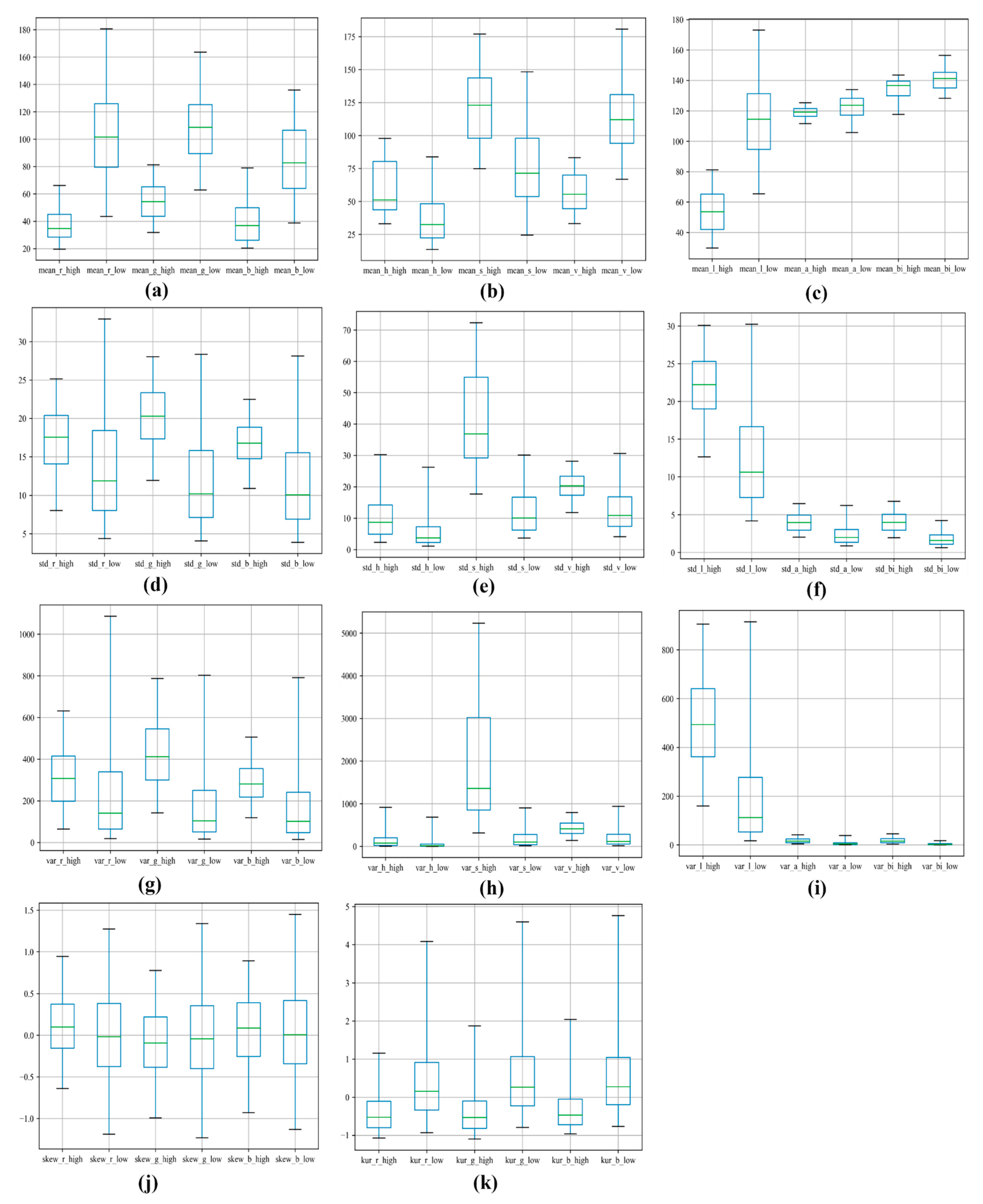
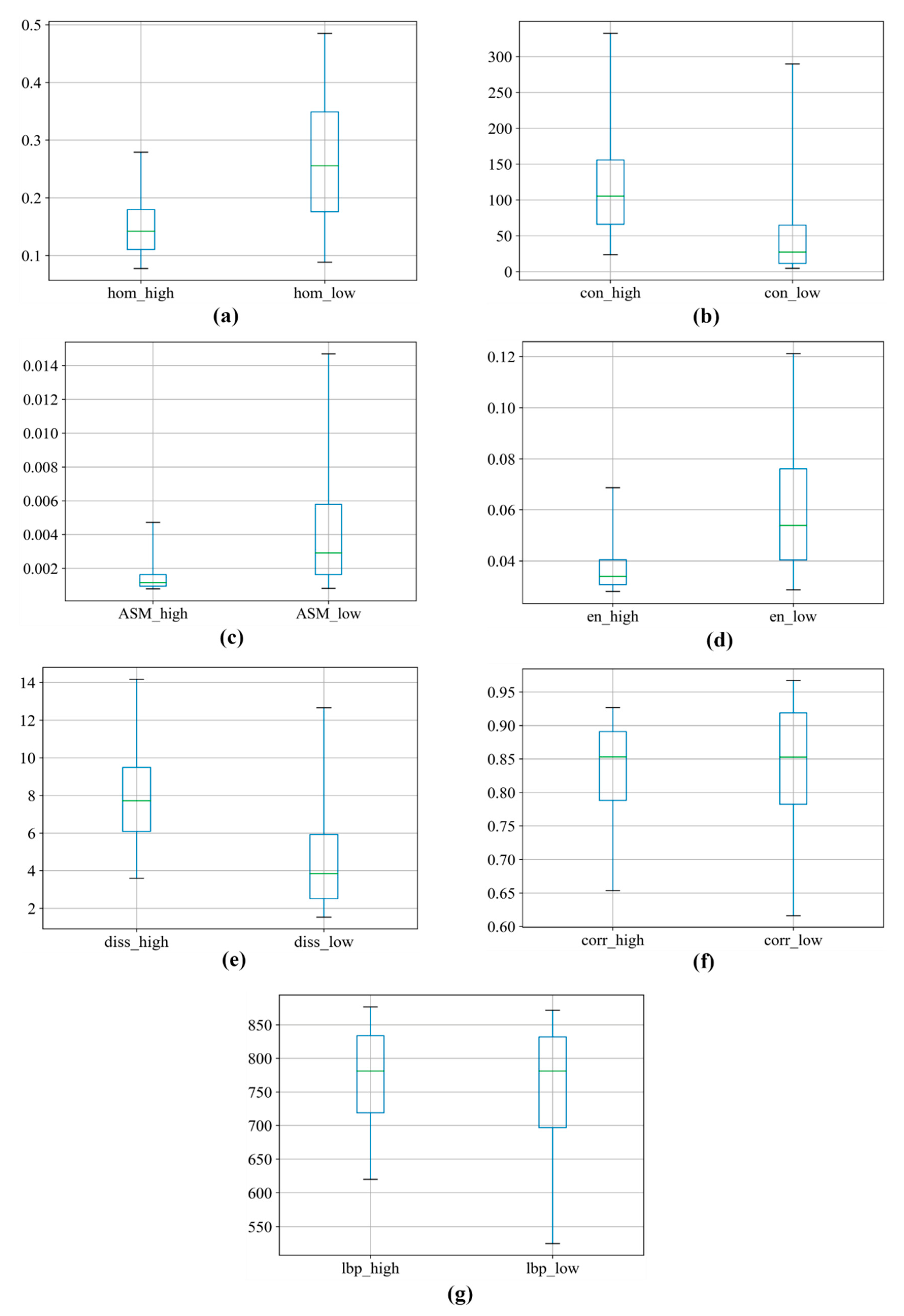
2.2. Feature Extraction

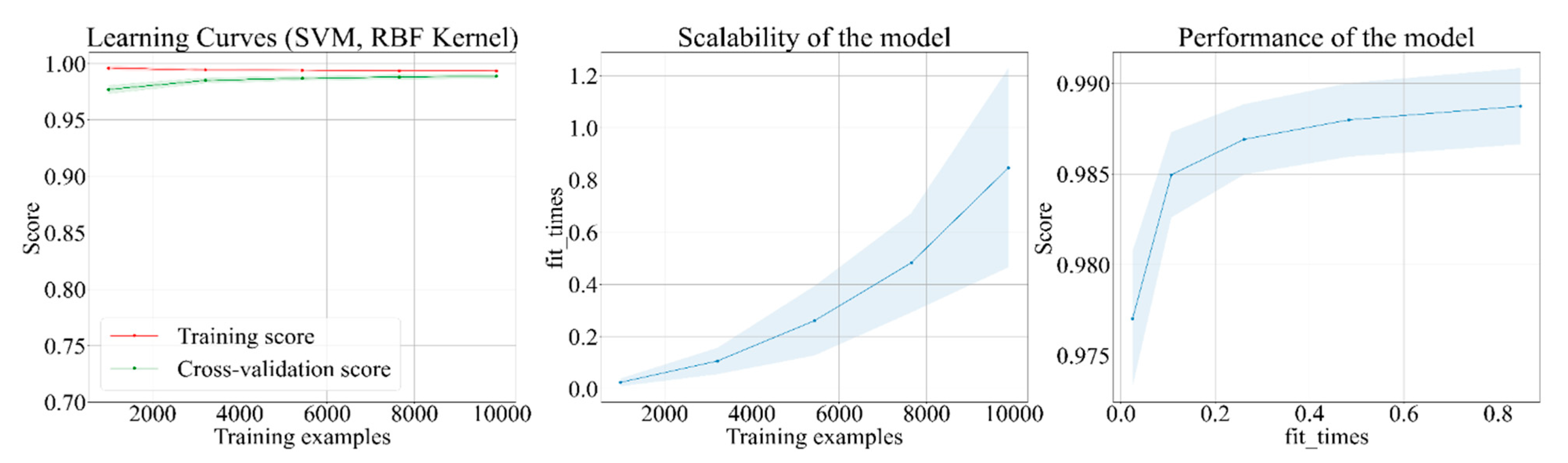
The process of analyzing and selecting features from satellite images datasets is a challenging task. A study by Berberoğlu et al. [17] assessed the incorporation of spatial and spectral features. The study used the variogram texture feature which was extracted from the gray level co-occurrence matrix (GLCM) on six bands of Landsat TM satellite imagery to classify the land-cover areas. A study by Li et al. [18] used a combination of vegetation index features and image texture features to identify vegetation regions. The texture features included the GLCM features and the local binary pattern (LBP) feature. On the other hand, the vegetation index features included the NDVI, radio vegetation index (RVI), and perpendicular vegetation index (PVI). The authors used the SVM algorithm for the classification process and the study concluded that the mean value of the NDVI represents the most effective feature. Additionally, a similar study by Iovan et al. [19] extracted the GLCM texture features from three color spaces: hue saturation and value (HSV) color space, XYZ color space, and the CEILAB color space, for two types of images: the first type was the high-resolution color infrared (CIR) and the second the digital surface model image. The study concluded that the GLCM features which were extracted from the HSV color space achieved the best classification accuracy of 95.84%. However, multispectral satellite data can increase the cost of the monitoring process. Based on the previous works on vegetation detection from satellite images, we divided the input features into two categories: color-based features and textural-based features. The color features consist of the statistical moments of three types of color spaces, which are: the RGB color space, the HSV color space, and the CIELAB color space, where the color space is the mathematical representation of colors in different dimensions [20]. In contrast, the textural-based features consist of the GLCM features, which are: homogeneity, energy, contrast, dissimilarity, correlation, and angular second moment. The statistical moments were calculated after flattening the patch image into a one-dimensional vector shape. The statistical moments are described in (1) to (6) [21,22].

$$\mu =\frac{{{\displaystyle \sum }}_{i=0}^{N-1}{p}_i}{N}$$

(1)

$${\sigma }^2=\frac{{{\displaystyle \sum }}_{i=0}^N{\left(p_i-\mu \right)}^2}{N}$$

(2)

$$\sigma =\sqrt{{\sigma }^2}$$

(3)

$${\mu }_k={\displaystyle \sum }_{i=0}^{N-1}{\left(p_i-\mu \right)}^k$$

(4)

$${\tilde{\mu }}_3=\frac{{\mu }_3}{{\sigma }^3}$$

(5)

$$Kurt\left[p_i\right]=\frac{{\mu }_4}{{\sigma }^4}$$

(6)

where µ, σ, σ², ${\tilde{\mu }}_3$, and Kurt are the mean, standard deviation, variance, skewness, and kurtosis moments, respectively. N is the vector length and P_i is the vector element. The textural features have properties that are not affected by the color values. The GLCM describes the frequent occurrence of values in a specific direction as illustrated in Figure 4. This method gives an impression of the relationship between neighboring pixel values [23]. In this work, we extracted the GLCM at a fixed angle of zero degrees. The GLCM features are the features which were extracted from the GLCM map. In this work, the extracted GLCM features are described in (7) to (12) [23,24]. Figure 5 and Figure 6 show the boxplot analysis of the statistical moments of the color spaces and the texture features. The boxplots (b), (e), and (f) in Figure 6 which are the contrast dissimilarity and correlation, respectively, show indistinct differences in the range of values between high- and low-density classes.

$$contrast={\displaystyle \sum }_{i,j=0}^{N-1}{p}_{i,j}{\left(i-j\right)}^2$$

(7)

$$energy={\displaystyle \sum }_{i,j=0}^{N-1}{p}_{i,j}{}^2$$

(8)

$$homogeneity=\frac{{{\displaystyle \sum }}_{i,j=0}^{N-1}{p}_{i,j}}{1+{\left(i-j\right)}^2}$$

(9)

$$correlation={\displaystyle \sum }_{i,j=0}^{N-1}{p}_{i,j}\left|\frac{\left(i-{\mu }_i\right)\left(j-{\mu }_j\right)}{\sqrt{({\sigma }_i^2)({\sigma }_j^2)}}\right|$$

(10)

$$angular second moment={\displaystyle \sum }_i{\displaystyle \sum }_j{\left(p_{i,j}\right)}^2$$

(11)

$$dissimilarity={\displaystyle \sum }_{i,j=0}^{N-1}{p}_{i,j}\left|i-j\right|$$

(12)

In addition to the GLCM features, the LBP feature was also used as an additional textural feature. The LBP is used in many applications such as face recognition and texture analysis [25,26]. The basic concept of the LBP is to convert the gray level image into a set of labels. The labels are constructed by creating a binary image by taking the threshold value from a center pixel point against a set of neighboring pixels, usually 3 × 3 pixels, then converting the binary values into a decimal gray level representation [25]. Figure 7 shows the conversion steps of the LBP image.

The LBP labeled image contains a two-dimensional integer matrix which can be impractical for use as a feature, while the rest of the features have a scalar representation.

As an abstraction, we used the sum of all binary values as a single scalar value to represent the LBP feature. This feature can be described as the sum of the LBP.

2.3. SVM Training

The SVM [27,28] has been used in a wide range of applications. The problems that the SVM algorithm can solve are related to statistical problems such as regression and classification problems. Figure 8 represents a simple linear classification problem where there are two features and two classes that are annotated with blue and red, respectively. The output of the SVM classifier is one of the labeled classes. The process of training the SVM model involves finding the optimal slope of the hyperplane and the largest possible margin that can separate the data with respect to the number of classes, as shown in Figure 8. The hyperplane equation can be described as in (13) where ω determines the slope of the plane, b is the bias value, and x is the input feature vector. The optimal margin width can be determined by the nearest data points from the hyperplane which are called the support vectors, as shown in Figure 8. The purpose of the margin function is to predict the output class for every new data point, as in (14) where ỹ is the predicted class.

$${\omega }^T.\overline{x}+b=0$$

(13)

$$\tilde{y}\{\begin{array}{c}0, if{\omega }^T.\overline{x}+b<0\\ 1, if {\omega }^T.\overline{x}+b\ge 0\end{array}$$

(14)

The ability of machine learning algorithms to learn corresponds to the ability of minimizing the error loss. In the SVM, the process of maximizing the margin is proportional to minimizing error loss. There are two types of margins: soft and hard. The hard margin is the optimal case where no data points are allowed inside the margin. On the other hand, the soft margin allows a few margin violations, which provides more dynamic classification to avoid overfitting. The number of points that can violate the margin can be regulated by a margin error cost c parameter where a larger c value means fewer margin violations. However, not all classification problems can be solved using linear models. A kernelized SVM version can be used to transform the classification problems into higher dimensions, resulting in non-linear transformations. The SVM algorithm has several kernels for solving different types of classification complexity. Equations (15)–(18) show the SVM kernels used in this study, which are: linear, Gaussian radial basis function (RBF), polynomial kernels, and sigmoid [27,28].

$$linear=k\left(x,x_i\right)={\left(x\right)}^T.\left(x_i\right)$$

(15)

$$Gaussian RBF=k\left(x,x_i\right)=exp\left(-\gamma \Vert x-x_i\Vert {}^2\right)$$

(16)

$$polynomial=k\left(x,x_i\right)={\left(\gamma x^T.x_i+r\right)}^d$$

(17)

$$\mathrm{sigmoid}=\mathrm{k}\left(\mathrm{x},{\mathrm{x}}_{\mathrm{i}}\right)=\tanh \left({\mathsf{\gamma }\mathrm{x}}^{\mathrm{T}}.{\mathrm{x}}_{\mathrm{i}}+\mathrm{r}\right)$$

(18)

$$\mathrm{standard}\mathrm{value}=\frac{\left({\mathrm{x}}_{\mathrm{i}}-\mathrm{mean}\right)}{\mathrm{STD}}$$

(19)

The symbol (x, x_i) is the data elements, γ is a parameter, d is the polynomial order, and r is a constant. The input feature vector was scaled using (19) to enhance the fitting process. Parameter optimization algorithms can be used to set the optimal values of the kernel parameters and the error cost parameter in order to achieve the best performance. In this work, the grid search algorithm [29] has been used to optimize the parameters of four SVM kernels and the corresponding margin error cost parameter for every kernel, as shown in

Table 1. SVM kernel parameter optimization.

	Parameter
Kernel	C	γ	r	d	Cross-Validation Recall Accuracy
Linear	10	-	-	-	0.96421
RBF	100	0.01	-	-	0.98274
Polynomial	1000	0.01	1	2	0.98003
Sigmoid	1000	-	0	-	0.86830

. The grid search algorithm has two steps, firstly, a grid of parameters values is proposed by the user, and secondly, the grid search algorithm uses the k-fold cross-validation technique to evaluate the performance of all the possible parameter combinations. The best cross-validation performance achieved by the RBF kernel is shown in Table 1. Figure 9 represents the training metrics of the SVM algorithm with the optimized Gaussian RBF kernel. Despite the large value of the error cost parameter, the cross-validation curve proves that there is no overfitting as the testing results are very close to the training results.

Additionally, Figure 9 describes the scalability and the performance of the trained SVM model. The scalability curve measures the ability of the trained model to be scaled using many workstations to deal with a large amount of input data without losing the classification performance. The recall accuracy can be described as the number of total true positive labels TP over the sum of the total true positive labels and false negative FN labels, as shown in (20) [30].

$$recall=\frac{TP}{TP+FN}$$

(20)

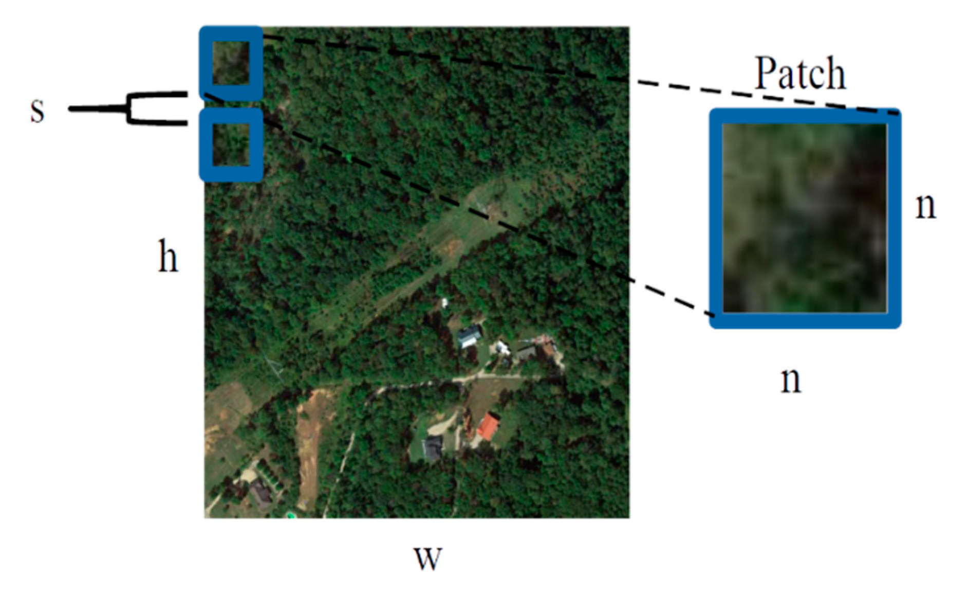
2.4. Automatic Patch Extraction

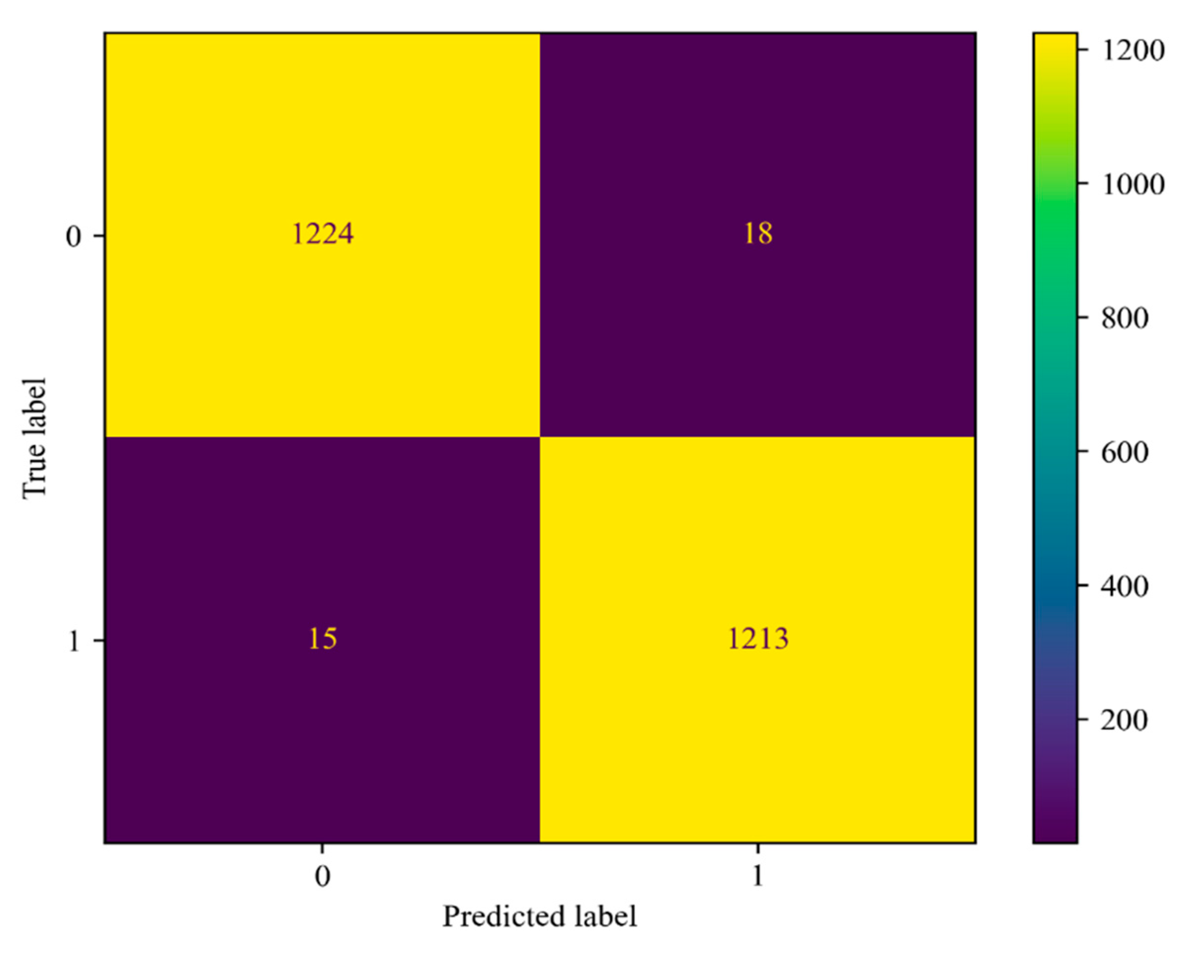
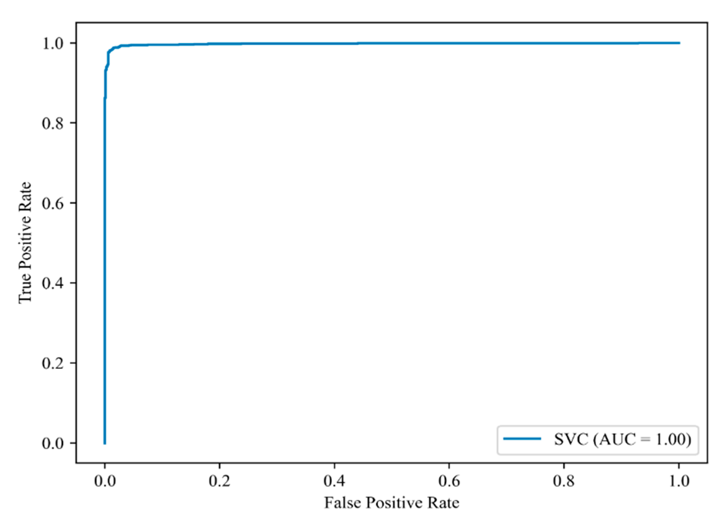
The input image was divided into n × n-pixels patches where the total number of patches N represents the total segments.

$$N=\lfloor {(\frac{w}{n+s})}^2\rfloor$$

(21)

$$N=\lfloor \left(\frac{w}{n+s}\right)+\left(\frac{h}{n+s}\right) \rfloor$$

(22)

If the input image has a square shape, the width w and the height h are equal. The total number of patches N can be calculated as in (21). The offset between patches s controls the density of the patches as shown in Figure 10. If the input image is not square, then the number of patches N can be described as in (22).

The process of dividing the image into small patches aims to reduce the processing time. However, the detection time is proportional to the number of sliced patch images, where more images require more execution time.

Table 2. SVM kernel parameter optimization.

1300 × 1300-Pixel Image
Patch Size (Pixel)	Slicing Time (s)	Feature Extraction + Classification Time (s)	Total Detection Time (s)
128 × 128	0.442927	9.429314	9.872241
64 × 64	0.818342	12.76653	13.58487
32 × 32	2.415230	18.02610	20.44133
16 × 16	82.29790	111.42492	193.7228

shows the relation between patch size, image slicing time, and classification time in seconds. However, the patch should have a reasonable size, for example, a patch size of 4 × 4 pixels cannot be used due to the poor-quality extracted values. Figure A1 shows an examples of vegetation encroachment detection with different patch sizes.

3. Results

In this section, we will discuss the performance when using different feature configurations and the corresponding detection results.

After training the SVM model, the model was tested on a new subset of data and Figure 11 shows the SVM testing confusion matrix. The trained SVM model achieved a testing recall classification accuracy of 98.55% for the low-density vegetation class and 98.78% for the high-density vegetation class. Figure 12 shows the SVM receiver operating characteristic (ROC) curve of the support vector classifier (SVC), where AUC represents the area under the curve. As illustrated previously in Figure 5 and Figure 6, there were some features that did not have any apparent difference in range between high- and low-density vegetation patches. These features can affect the classification accuracy.

Table 3. Recall accuracy of the proposed model compared with different feature configurations.

	Cross-Validation Recall Accuracy
Feature	SVM (Poly)	SVM (Linear)	SVM (RBF)	SVM (Sigmoid)
Statistical moment of the RGB color space	0.96906	0.95975	0.96760	0.83979
Statistical moment of the RGB color space + skew moment + kurtosis moment	0.97586	0.96291	0.97513	0.83469
Statistical moment of the HSV color space	0.96469	0.95594	0.96478	0.88515
Statistical moment of the CIELAB	0.96833	0.94792	0.96898	0.87332
Statistical moment of the RGB color space + statistical moment of the HSV color space	0.97359	0.96285	0.97424	0.84879
LBP feature	0.54291	0.53562	0.54331	0.45829
GLCM features	0.81687	0.77013	0.81736	0.66287
GLCM features + LBP feature	0.84453	0.79393	0.844534	0.64049
GLCM features + statistical moment of the RGB color space + statistical moment of the HSV color space + statistical moment of the CIELAB color space	0.97617	0.97449	0.97935	0.88700
Selected features	0.9800	0.96421	0.98274	0.86830

shows the cross-validation performance of different feature configurations.

As observed from Table 3, some features are essential to increase the classification accuracy, such as the RGB statistical moments and the HSV statistical moments. However, not all the GLCM features are effective.

We selected only the most effective GLCM features, which were: homogeneity, ASM, and energy. In addition, we used the LBP as we observed an enhancement in the cross-validation recall accuracy when we used the LBP feature with the GLCM features, as shown in Table 3. The selected features represent the total effective features, which were: the statistical moments of the RGB color space, the statistical moments of the HSV color space, homogeneity, ASM, energy, and the LBP. Figure 13 shows an example of the proposed vegetation density classification result around the power line corridor ROW, where the green regions represent the low-density vegetation patches and the red regions represent the high-density vegetation patches. The recall accuracy of the SVM classifier was compared to other machine learning classifiers, which were: tree, random forest, k- nearest neighbor (KNN) and naïve Bayes, as shown in Figure 14. All the machine learning classifiers were optimized and evaluated with the best performance against the SVM (RBF kernel), where the SVM classifier scored the best recall accuracy of 98.274%.

Despite the effectiveness of the visible light band on the vegetation density classification accuracy, the topography of the land plays a major role in deviating the reflected electromagnetic wave from the Earth’s surface. A heterogeneous surface affects the anisotropy of the reflected electromagnetic solar irradiance due to the diffusion between the terrain slopes, which can provide a deviated pixel value [31]. However, this effect can be analyzed at the macro- and micro-level using different methods. The diffused equivalent slope model (dESM) is one of the proposed solutions to simulate and analyze the effect of the micro-slope on the anisotropy reflectance under different illumination conditions, which can help to evaluate the level of pixel value deviation [32].

4. Conclusions

In this paper, we discussed the effect of using color and texture features to classify the vegetation density along the power line corridor ROW from the visible light band of high-resolution satellite images into two classes of high- and low-density vegetation. We proposed to use only the most effective features by analyzing the behavior of both color and texture features. The results showed that there were some features that reduced the classification accuracy, which were: the CIELAB statistical moments, correlation, dissimilarity, and contrast. The proposed feature configurations gave the best result among the other configurations, where the recall classification accuracy was 98.272% using the SVM RBF kernel. The results emphasize the possibility of using satellite images with the visible light band only to detect the vegetation encroachment along the power line ROW. The limitation of the study was the inability to identify tree heights around the power line corridor.

References

1. Alhelou, H.H.; Hamedani-Golshan, M.E.; Njenda, T.C.; Siano, P. A Survey on Power System Blackout and Cascading Events: Research Motivations and Challenges. Energies 2019, 12, 682. [Google Scholar] [CrossRef] [Green Version]
2. Gomes-Mota, J.; Brantes, A.; Pinto, L.C.; De Exploracao, D.; Azevedo, F. How environmental factors impact line performance, field results from Southwest Europe. In Proceedings of the 2012 11th International Conference on Environment and Electrical Engineering, Venice, Italy, 18–25 May 2012; pp. 1053–1058. [Google Scholar] [CrossRef]
3. Haroun FM, E.; Deros SN, M.; Din, N.M. A review of vegetation encroachment detection in power transmission lines using optical sensing satellite imagery. Int. J. Adv. Trends Comput. Sci. Eng. 2020, 9, 618–624. [Google Scholar] [CrossRef]
4. Ahmad, J.; Malik, A.S.; Xia, L.; Ashikin, N. Vegetation encroachment monitoring for transmission lines right-of-ways: A survey. Electr. Power Syst. Res. 2013, 95, 339–352. [Google Scholar] [CrossRef]
5. Matikainen, L.; Lehtomäki, M.; Ahokas, E.; Hyyppä, J.; Karjalainen, M.; Jaakkola, A.; Kukko, A.; Heinonen, T. Remote sensing methods for power line corridor surveys. ISPRS J. Photogramm. Remote Sens. 2016, 119, 10–31. [Google Scholar] [CrossRef] [Green Version]
6. Ahmad, J.; Malik, A.S.; Xia, L. Effective techniques for vegetation monitoring of transmission lines right-of-ways. In Proceedings of the 2011 IEEE International Conference on Imaging Systems and Techniques, Batu Ferringhi, Malaysia, 17–18 May 2011; pp. 34–38. [Google Scholar]
7. Agrawal, S.; Khairnar, G.B. A comparative assessment of remote sensing imaging techniques: Optical, sar and lidar. ISPRS Int. Arch. Photogramm. Remote Sens. Spat. Inf. Sci. 2019, 42, 1–6. [Google Scholar] [CrossRef] [Green Version]
8. Purnamasayangsukasih, P.R.; Norizah, K.; Ismail, A.A.M.; Shamsudin, I. A review of uses of satellite imagery in monitoring mangrove forests. IOP Conf. Ser. Earth Environ. Sci. 2016, 37, 012034. [Google Scholar] [CrossRef]
9. Liu, G.-R.; Liang, C.-K.; Kuo, T.-H.; Lin, T.-H.; Huang, S.-J. Comparison of the NDVI, ARVI and AFRI Vegetation Index, Along with Their Relations with the AOD Using SPOT 4 Vegetation Data. Terr. Atmos. Ocean. Sci. 2004, 15, 15–31. [Google Scholar] [CrossRef] [Green Version]
10. Mikhalap, S.; Trashenkov, S.; Vasilyeva, V. Study of overhead power line corridors on the territory of pskov region (russia) based on satellite sounding data. Vide. Tehnol. Resur. Environ. Technol. Resour. 2019, 1, 164–167. [Google Scholar] [CrossRef]
11. Jardini, M.G.M.; Jardini, J.A.; Magrini, L.C.; Masuda, M.; Le Silva, P.R.; Quintanilha, J.A.; Beltrame, A.M.K.; Jacobsen, R.M. Vegetation Control of Transmission Lines Right-of-way. In Proceedings of the 2007 3rd International Conference on Recent Advances in Space Technologies, Istanbul, Turkey, 14–16 June 2007; pp. 660–665. [Google Scholar]
12. Kwan, C.; Gribben, D.; Ayhan, B.; Li, J.; Bernabe, S.; Plaza, A. An Accurate Vegetation and Non-Vegetation Differentiation Approach Based on Land Cover Classification. Remote Sens. 2020, 12, 3880. [Google Scholar] [CrossRef]
13. Kaufman, Y.J.; Tanre, D. Atmospherically Resistance Vegetation Index (ARVI) for EOS-MODIS. IEEE Trans. Geosci. Remote Sens. 1992, 30, 261–270. [Google Scholar] [CrossRef]
14. Kobayashi, Y.; Karady, G.G.; Heydt, G.T.; Olsen, R.G. The Utilization of Satellite Images to Identify Trees Endangering Transmission Lines. IEEE Trans. Power Deliv. 2009, 24, 1703–1709. [Google Scholar] [CrossRef]
15. Moeller, M.S. Monitoring Powerline Corridors with Stereo Satellite Imagery. In Proceedings of the MAPPS/ASPRS Conference, San Antonio, TX, USA, 6–10 November 2006; pp. 1–6. Available online: http://www.asprs.org/a/publications/proceedings/fall2006/0034.pdf (accessed on 1 June 2021).
16. Aqeel, M.; Jamil, M.; Yusoff, I. Introduction to Remote Sensing of Biomass. In Biomass and Remote Sensing of Biomass; IntechOpen: Beijing, China, September 2011; pp. 129–169. Available online: https://www.intechopen.com/books/biomass-and-remote-sensing-of-biomass/introduction-to-remote-sensing-of-biomass (accessed on 1 June 2021). [CrossRef] [Green Version]
17. Berberoglu, S.; Akin, A.; Atkinson, P.M.; Curran, P.J. Utilizing image texture to detect land-cover change in Mediterranean coastal wetlands. Int. J. Remote Sens. 2010, 31, 2793–2815. [Google Scholar] [CrossRef] [Green Version]
18. Li, Z.; Hayward, R.; Zhang, J.; Jin, H.; Walker, R. Evaluation of Spectral and Texture Features for Object-Based Vegetation Species Classification Using Support Vector Machines. In Proceedings of the ISPRS TC VII Symp—100 Years ISPRS, Vienna, Austria, 5–7 July 2010; pp. 122–127. Available online: http://www.isprs.org/proceedings/XXXVIII/part7/a/pdf/122_XXXVIII-part7A.pdf (accessed on 1 June 2021).
19. Iovan, C.; Boldo, D.; Cord, M. Detection, Segmentation and Characterisation of Vegetation in High-Resolution Aerial Images for 3D City Modelling. Int. Arch. Photogramm. Remote Sens. Spat. Inf. Sci. 2008, 36, 247–252. [Google Scholar]
20. Ganesan, P.; Rajini, V. Assessment of satellite image segmentation in RGB and HSV color space using image quality measures. In Proceedings of the 2014 International Conference on Advances in Electrical Engineering (ICAEE), Vellore, India, 9–11 January 2014. [Google Scholar]
21. Shijin Kumar, P.S.; Dharun, V.S. Extraction of Texture Features using GLCM and Shape Features using Connected Regions. Int. J. Eng. Technol. 2016, 8, 2926–2930. [Google Scholar] [CrossRef] [Green Version]
22. Liang, Z.; Wei, J.; Zhao, J.; Liu, H.; Li, B.; Shen, J.; Zheng, C. The statistical meaning of kurtosis and its new application to identification of persons based on seismic signals. Sensors 2008, 8, 5106–5119. [Google Scholar]
23. Haryanto, T.; Pratama, A.; Suhartanto, H.; Murni, A.; Kusmardi, K.; Pidanic, J. Multipatch-GLCM for Texture Feature Extraction on Classification of the Colon Histopathology Images using Deep Neural Network with GPU Acceleration. J. Comput. Sci. 2020, 16, 280–294. [Google Scholar] [CrossRef] [Green Version]
24. Suresh, A.; Shunmuganathan, K.L. Image texture classification using gray level co-occurrence matrix based statistical features. Eur. J. Sci. Res. 2012, 75, 591–597. [Google Scholar]
25. Zhou, W.; Ahrary, A.; Kamata, S.-I. Image Description with Local Patterns: An Application to Face Recognition. IEICE Trans. Inf. Syst. 2012, E95-D, 1494–1505. [Google Scholar] [CrossRef] [Green Version]
26. Yuan, J.-H.; Huang, D.-S.; Zhu, H.-D.; Gan, Y. Completed hybrid local binary pattern for texture classification. In Proceedings of the 2014 International Joint Conference on Neural Networks (IJCNN), Beijing, China, 6–11 July 2014; pp. 2050–2057. [Google Scholar]
27. Boser, B.E.; Guyon, I.M.; Vapnik, V.N. A training algorithm for optimal margin classifiers. In Proceedings of the Fifth Annual Workshop on Computational Learning Theory, Pittsburgh, PA, USA, 27–29 July 1992; pp. 144–152. [Google Scholar]
28. Corinna, C.; Vapnik, V. Support-Vector Networks. Mach. Learn. 1995, 20, 273–297. [Google Scholar]
29. Shekar, B.H.; Dagnew, G. Grid Search-Based Hyperparameter Tuning and Classification of Microarray Cancer Data. In Proceedings of the 2019 Second International Conference on Advanced Computational and Communication Paradigms (ICACCP), Gangtok, India, 25–28 February 2019; pp. 1–8. [Google Scholar] [CrossRef]
30. Goutte, C.; Gaussier, E. A probabilistic interpretation of precision, recall and F-score, with implication for evaluation. Lect. Notes Comput. Sci. 2005, 3408, 345–359. [Google Scholar]
31. Proy, C.; Tanré, D.; Deschamps, P.Y. Evaluation of topographic effects in remotely sensed data. Remote Sens. Environ. 1989, 30, 21–32. [Google Scholar] [CrossRef]
32. Hao, D.; Wen, J.; Xiao, Q.; Wu, S.; Lin, X.; You, D.; Tang, Y. Modeling Anisotropic Reflectance Over Composite Sloping Terrain. IEEE Trans. Geosci. Remote Sens. 2018, 56, 3903–3923. [Google Scholar] [CrossRef]
Figure 1. Low- and high-density vegetation encroachment on the power line corridor right-of-way (ROW).
Energies 14 03393 g001
Figure 2. The electromagnetic reflectance from the Earth’s surface of different elements [16].
Energies 14 03393 g002
Figure 3. Proposed vegetation encroachment detection method comprising of two stages: training and testing.
Energies 14 03393 g003
Figure 4. The creation of the gray level co-occurrence matrix (GLCM) that describes the frequent occurrence of the gray level values at zero degrees.
Energies 14 03393 g004
Figure 5. Comparison of high- and low-density vegetation patches for color space statistical moments where (ac) are the mean values of the color spaces, (df) are the standard deviations of the color spaces, (gi) are the variances of the color spaces, and (j,k) are the skew and kurtosis of the RGB color space.
Energies 14 03393 g005
Figure 6. Comparison of the high- and low-density vegetation patches for GLCM texture features where (a) is the homogeneity, (b) is the contrast, (c) is the angular second moment (ASM), (d) is the energy, (e) is the dissimilarity, (f) is the correlation, and (g) is the LBP.
Energies 14 03393 g006
Figure 7. Local binary pattern (LBP) conversion process where (a) is the RGB satellite image, (b) is the gray level image, and (c) is the LBP image.
Energies 14 03393 g007
Figure 8. Two-dimensional support vector machine (SVM).
Energies 14 03393 g008
Figure 9. Training metrics of the optimized SVM classifier with a radial basis function (RBF) kernel.
Energies 14 03393 g009
Figure 10. The process of patch creation where n is the patch width and height, w is the image width, h is the image height, and s is the step between patches.
Energies 14 03393 g010
Figure 11. SVM testing confusion matrix (RBF kernel).
Energies 14 03393 g011
Figure 12. SVM (RBF kernel) receiver operating characteristic (ROC) curve.
Energies 14 03393 g012
Figure 13. Examples of the vegetation density classification results along the power line corridor area with a patch size of 32 × 32-pixels and step size of s = 4. The red regions represent high-density vegetation and the green regions represent low-density vegetation.
Energies 14 03393 g013
Figure 14. Recall accuracy comparison between SVM (RBF kernel) and other optimized machine learning classifiers.
Energies 14 03393 g014