Numerical Analysis of Transient Performance of Grounding Grid with Lightning Rod Installed on Multi-Grounded Frame

Abstract

In large substations, many lightning rods are installed on multi-grounded frames. The lightning rods, the frame, the grounding grid and the soil form a whole body, and the lightning current will be discharged from many grounding points. In this paper, based on the partial element equivalent circuit method, a numerical model, in the time domain, is developed to simulate the lightning-caused electromagnetic transients on the frame and the grounding grid. The model is verified by field testing and by comparison with commercial software. The model has several features: (1) it has a simple time domain form; (2) it is stable due to a staggered arrangement of space and time variables and an implicit difference scheme used, and (3) the dimension of the equations is relatively small because the unknown variables are divided into several groups, which are calculated one by one. With this method, the transient characteristics of the grounding grid with lightning rods on the frame are calculated, and the factors affecting the results are analyzed. It can be seen that although the frame causes the ground potential rise in an evenly distributed manner, compared with the situation in which the lightning strikes an independent lightning rod, the ground potential decrease rate near the main grounding point is almost the same because most of the current still enters the soil from the grounding electrode closest to the lightning strike. Therefore, even if there is a frame, the nearby facilities should take the same protective measures as in the case of an independent lightning rod. The ground conductors near the grounding points of the frame should be dense enough to reduce the potential gradient. The equipment should be kept at least 10 m away from the grounding point for lightning.

1. Introduction

The grounding grid is an important component for lightning protection [1,2]. The transient performance of grounding system has been a hot topic for a long time [3,4,5]. Usually, the performance is analyzed with the lightning current injected from an independent lightning rod that has just one grounding point. However, in substations, in order to save space, many lightning rods are installed on the frames that were originally used to hang the overhead transmission lines. Since the frames have many legs and all of them are grounded, the lightning current will be distributed along the frame and be discharged from many grounding points. In this situation, the lightning rods, the frame, the grounding grid and the soil form a complex overall structure. Hence, it is interesting to analyze the transient characteristics of the grounding grid with lightning current injected from multi-grounded frames.

Usually, numerical EM-field methods can be used to simulate the frame and grounding grid as a whole. Among these methods, the electric-field integral-equation (EFIE) method based on moment methods (MoM) has been widely used due to the thin-wire structures of the frame and the grounding grid [6,7,8,9,10,11]. Alemi and Grcev, respectively, developed wide-band models of grounding systems based on MoM [6,7]. However, the EFIE method is usually developed in the frequency domain. In order to analyze the situation in the time domain, a fast Fourier transform is necessary [8,9]. There were also studies in the literature that used an impedance matrix or a generalized pencil of function to transform the parameters in the frequency domain into those in the time domain [10,11]. For lightning transient analysis, the time domain method is more convenient. Then, the finite-difference time domain (FDTD) method was adopted [12,13,14,15]. However, the structures to be simulated were usually simplified [12], and it is troublesome to build division meshes for irregular thin-wire structures. Recently, it has been verified that the partial element equivalent circuit (PEEC) method is quite effective in the evaluation of electromagnetic transients on thin-wire structures [16,17,18,19]. The method transforms the electromagnetic problem into a circuit that can be solved either in the frequency domain or in the time domain. Yutthagowith applied the PEEC method to analyze the transient potential rises in grounding systems [16]. Chen developed a PEEC method to analyze the grounding grid considering both the frequency-dependent behavior and ionization phenomenon [19]. However, when solving the circuit in the time domain, as the iteration steps increase, it becomes more and more difficult to ensure convergence [17]. In addition, in most papers, the authors either only focused on the above-ground facilities [5,13,14,18], or only focused on the grounding grid [4,6,7,8,11,15,16,19]. The above-ground and underground facilities are rarely considered together. In [9], the distribution of lightning current among interconnected grounding systems was calculated. Although it considered the interaction between the conductors above ground and those underground, its research object was different from that of this article, and it used the frequency domain method. In this paper, a time domain approach is developed based on the PEEC method. A staggered arrangement of space and time variables is introduced, for which the solution is very stable. Using this method, the transient characteristics of the grounding grid with lightning current injected from multi-grounded frames are analyzed.

This paper includes three parts. The first part introduces the basic principle of the approach. Then, verification of the approach is presented by comparing the calculated results with those obtained by field experiment, as well as by comparison with commercial software. Finally, the transient characteristics of the grounding grid with lightning rods on the frame are calculated. The main factors that affect the impulse grounding resistance and the ground potential distribution along the grounding grid are analyzed.

2. Basic Principle

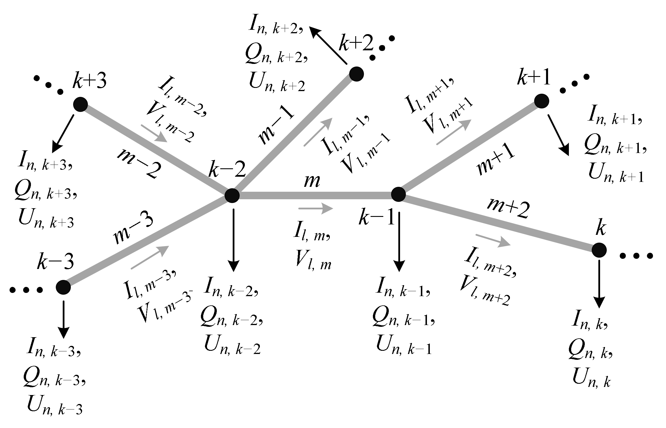
2.1. Coupling Mechanisms among Conductors

First, all the conductors of the grounding grid and frame are divided into short segments. According to the four coupling mechanisms among conductors, namely, capacitive coupling, conductive coupling, inductive coupling, and resistive coupling, the basic relationships between potentials, currents, and charges on the segments of the conductors can be established. Because the size of the frame and the grounding grid is usually much less than the wavelength of the main frequency of the lightning current, static field theory is used to compute the lumped parameters that represent the above relationship [16,17].

Based on the capacitive coupling and the conductive coupling among the segments, the potentials of the segments are determined by the charges on the segments and the current leaked from the segments, and following equation can be set up [17]:

$$U_n=R{I}_n=P{Q}_n,$$

(1)

where U_n is the vector of the potentials of the segments, Q_n is the vector of the charges bonded on the segments, and I_n is the vector of the radially conductive currents flowing out of the segments. P is a potential coefficient matrix, and R is a mutual resistance matrix.

Based on the conductive coupling and the inductive coupling among the segments, the potential drops along segments are determined by the longitudinal resistances and currents of the segments, as well as the mutual inductances among the segments, and hence, the following equation can be set up [17]:

$$V_l=R_l{I}_l+L\frac{d{I}_l}{dt},$$

(2)

where R_l is the matrix of the longitudinal resistance of the segments, which has only nonzero elements on its diagonal, and L is an inductance matrix, which is a full matrix with self-inductance on its diagonal and mutual inductance off its diagonal. V_l is the vector of the potential drops along the segments, and I_l is the vector of the segment currents whose positive direction is defined as that from the starting point of a segment to its end point.

For the segments in the air, corresponding elements in I_n are almost zero, and all the elements in corresponding rows and columns of R approach infinity, while, for the segments under the ground, I_n cannot be neglected. Let the parameters in the air be indicated by subscript 1 and those under the ground be indicated by subscript 2. In the air, (1) will become:

$$U_{n1}=P_{11}{Q}_{n1}+P_{12}{Q}_{n2},$$

(3)

While, under the ground, (1) will become:

$$U_{n2}=R_{22}{I}_{n2}=P_{21}{Q}_{n1}+P_{22}{Q}_{n2},$$

(4)

where R₂₂ is the mutual resistance matrix among the segments under the ground, and P₁₁, P₁₂, P₂₁, and P₂₂ are sub-matrices of P:

$$P=\left[\begin{array}{cc}{P}_{11}& P_{12}\\ P_{21}& P_{22}\end{array}\right],$$

(5)

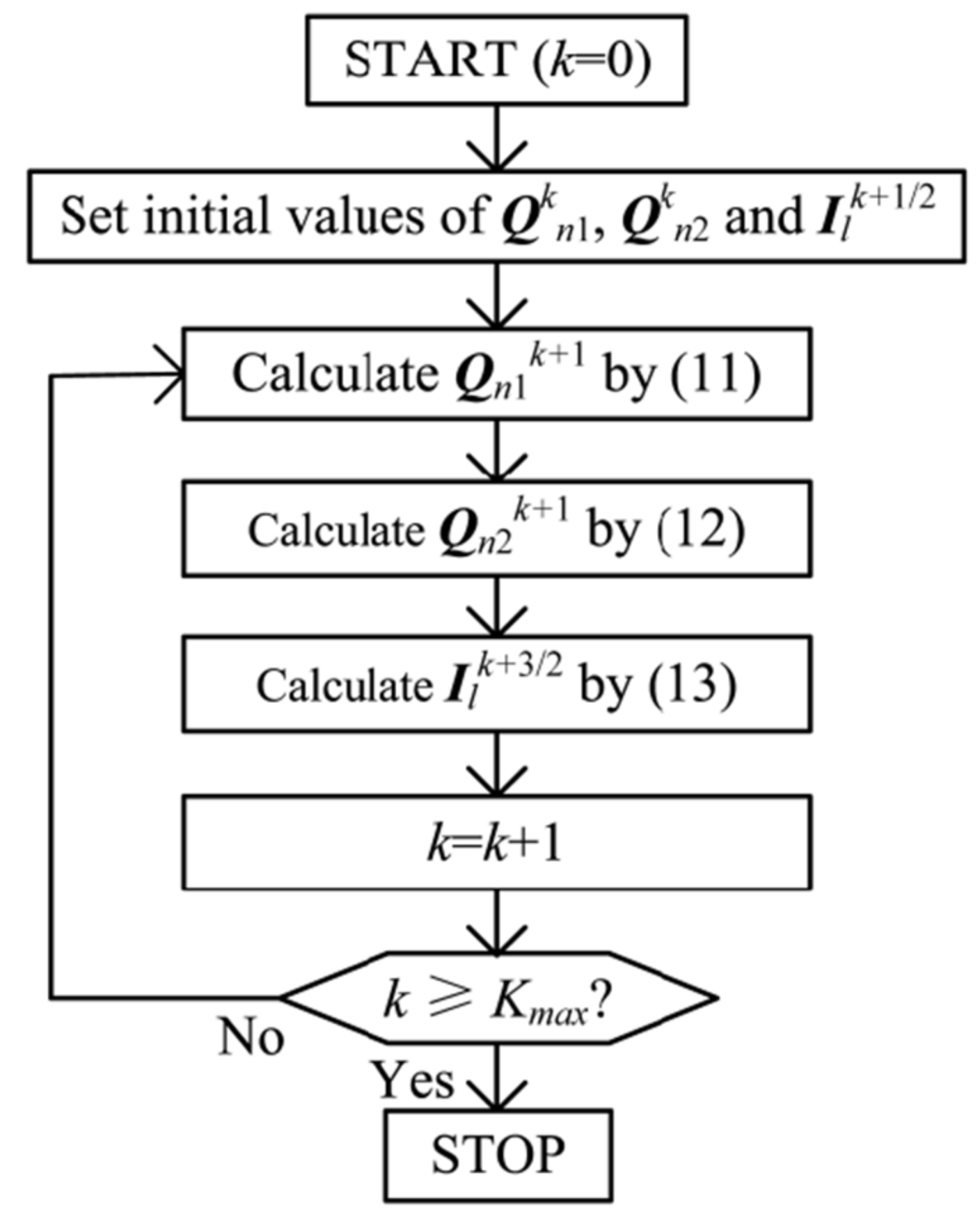
2.2. Node Potential Method in the Time Domain

Based on above coupling mechanisms, the electromagnetic field problem can be turned into a circuit problem. Because U_n denotes the potentials to infinity, if infinity is regarded as a reference point, it will be easy to set up equations by using the node potential method. Let the segments be branches and their intersections be nodes. Then, Q_n, U_n, and I_n can be arranged around the nodes, and I_l is along the segments, as Figure 1 shows, in which points k − 3 to k + 3 are nodes, and segments m − 3 to m + 2 are branches. According to Kirchhoff’s current law, the following equations can be obtained at the nodes:

$$A_1^T{I}_l+I_s=\frac{d{Q}_{n1}}{dt}, \mathrm{for} \mathrm{the} \mathrm{segments} \mathrm{in} \mathrm{the} \mathrm{air},$$

(6)

$$A_2^T{I}_l-I_{n2}=\frac{d{Q}_{n2}}{dt}, \mathrm{for} \mathrm{the} \mathrm{segments} \mathrm{under} \mathrm{the} \mathrm{ground},$$

(7)

where I_s is the lightning current matrix of the nodes above the ground. If a lightning strikes node i, I_si will be the lightning current, while other entries should be zeros. A₁ is the matrix of the connection relationship between the nodes in the air and all the segments, and A₂ is that between the nodes under the ground and all the segments. The elements of A₁ and A₂ are:

$$A_{ij}=\left\{\begin{array}{c}1,\mathrm{if} \mathrm{node} j \mathrm{is} \mathrm{connected} \mathrm{to} \mathrm{the} \mathrm{end} \mathrm{of} \mathrm{segment} i\\ -1,\mathrm{if} \mathrm{node} j \mathrm{is} \mathrm{connected} \mathrm{to} \mathrm{the} \mathrm{start} \mathrm{of} \mathrm{segment} i\\ 0,\mathrm{if} \mathrm{node} j \mathrm{is} \mathrm{not} \mathrm{directly} \mathrm{connected} \mathrm{to} \mathrm{segment} i\end{array}\right..$$

Since (7) has too many unknown variables, by substituting (4) into it, it will be turned into:

$$A_2^T{I}_l-R_{22}^{-1}(P_{21}{Q}_{n1}+P_{22}{Q}_{n2})=\frac{d{Q}_{n2}}{dt},$$

(8)

For the branches, let A = [A₁ A₂]. Since the potential difference between the two ends of the segment is the voltage drop of the segment, the voltage drops along the segments and the potentials at the nodes will have the following relationship:

$$V_l=-A{U}_n.$$

(9)

By substituting (1) into (9), and then into (2), we will get:

$$L\frac{d{I}_l}{dt}=-R_l{I}_l-AP{Q}_n,$$

(10)

Based on (6), (8), and (10), by using Q_n and I_l as unknown variables, the problem under consideration can be solved in the time domain with the help of a difference method. Since the time variation of I_l determines Q_n, while the time variation of Q_n determines I_l, a difference method can be introduced based on the idea of FDTD. That is, the charge and current are not only interleaved in space but also interleaved in time. For example, at the kth step, if $Q_n^k$ is at time kΔt while $I_l^{k+1/2}$ is at time (k + 1/2)Δt, and $Q_n^{k+1/2}$ is the average of $Q_n^k$ and $Q_n^{k+1}$ while $I_l^k$ is the average of $I_l^{k+1/2}$ and $I_l^{k-1/2}$, the following equations can be obtained:

$$Q_{n1}^{k+1}=Q_{n1}^k+\Delta t(A_1^T{I}_l^{k+1/2}+I_s^{k+1/2}),$$

(11)

$$Q_{n1}^{k+1}=Q_{n1}^k+\Delta t(A_1^T{I}_l^{k+1/2}+I_s^{k+1/2}),$$

(12)

$$\begin{gathered} I_l^{k+3/2}=I_l^{k+1/2}-\frac{\Delta t}{2}{L}^{-1}{R}_l(I_l^{k+3/2}+I_l^{k+1/2}) \\ -\Delta t{L}^{-1}A\left[\begin{array}{cc}{P}_{11}& P_{12}\\ P_{21}& P_{22}\end{array}\right]\left[\begin{array}{c}{Q}_{n1}^{k+1}\\ Q_{n2}^{k+1}\end{array}\right] \end{gathered}$$

(13)

Since $I_s$ is the lightning current, if $Q_{n1}^k$, $Q_{n2}^k$, and $I_l^{k+1/2}$ are known, the new values $Q_{n1}^{k+1}$ and $Q_{n2}^{k+1}$ can be obtained by solving (11) and (12). Then, $I_l^{k+3/2}$ can be calculated by solving (13). Thus, the transient performance of the frame and the grounding grid can be simulated in the time domain step by step. The whole procedure is displayed in Figure 2. Because the implicit difference scheme is used in (13), the calculation is stable. At the same time, because Q_n1, Q_n2 and I_l are calculated one by one, the dimension of the equations is relatively small.

2.3. Initial Values of Q_n and I_l

In order to start the calculation, the following method is used to set the initial values of Q_n and I_l. At the beginning, $Q_{n1}^0$, $Q_{n2}^0$, and $I_l^{-1/2}$ can be set as zeros. According to (13), $I_l^{1/2}$ should be zero. Then, $Q_{n1}^1$ can be obtained from (11) since the lightning current is known. With $Q_{n1}^1$ being known, $Q_{n2}^1$ can be obtained from (12). After that, $I_l^{3/2}$ can be calculated from (13). Then, the calculation can be continued according to the procedure shown in Figure 2.

2.4. Calculation of R, P and L

Suppose the leakage currents around the nodes are leaked evenly from all halves of the segments connected to the nodes, and then R_ij in R is equal to the potential at node i when a unit current is leaked evenly from all halves of the segments connected to node j. Thus, R_ij is the sum of the integrals of Green’s function from node j to the middle points of the segments connected to node j. For example, R_ik at node i, caused by the leakage current I_{n, k} from node k in Figure 1, can be calculated by:

$$R_{ik}=\frac{1}{l_m+l_{m+1}+l_{m+2}}\left(l_m{\displaystyle {\int }_0^{l_m/2}{G}_m\left(r\right)d{l}_m}+l_{m+1}{\displaystyle {\int }_0^{l_{m+1}/2}{G}_{m+1}\left(r\right)d{l}_{m+1}}+l_{m+2}{\displaystyle {\int }_0^{l_{m+2}/2}{G}_{m+2}\left(r\right)d{l}_{m+2}}\right)$$

(14)

where l_m, l_m+1, and l_m+2 are the lengths of segments m, m + 1 and m + 2, respectively, r is the distance between node j and the integral point, and G_m, G_m+1, and G_m+2 are the Green’s functions of corresponding segments, which are related to the locations of both node i and the segments in the air or soil, as well as the resistivity of the soil, and can be obtained by means of the image method [20].

Since the electric field generated by charge is similar to that generated by current, the above method is also suitable for calculating P.

The mutual inductance between segments can be obtained by:

$$L_{ij}=\frac{{\mu }_0}{4\pi }{\displaystyle {\int }_{l_j}({\displaystyle {\int }_{l_i}\frac{1}{r}d{l}_i})\times d{l}_j}$$

(15)

where l_i and l_j are the length vectors of segments i and j that are in the same directions as the corresponding axial currents. It should be noted that the soil and the air usually have the same permeability. If the two permeabilities are different, the image method is also needed in the calculation.

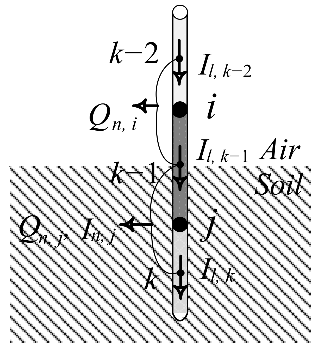
2.5. Segments at the Interface between the Air and the Soil

In order to make the current from the air to the soil continuous, at the interface, the conductor should be divided in the manner shown in Figure 3. That is, the segment should be just across the interface.

3. Verification

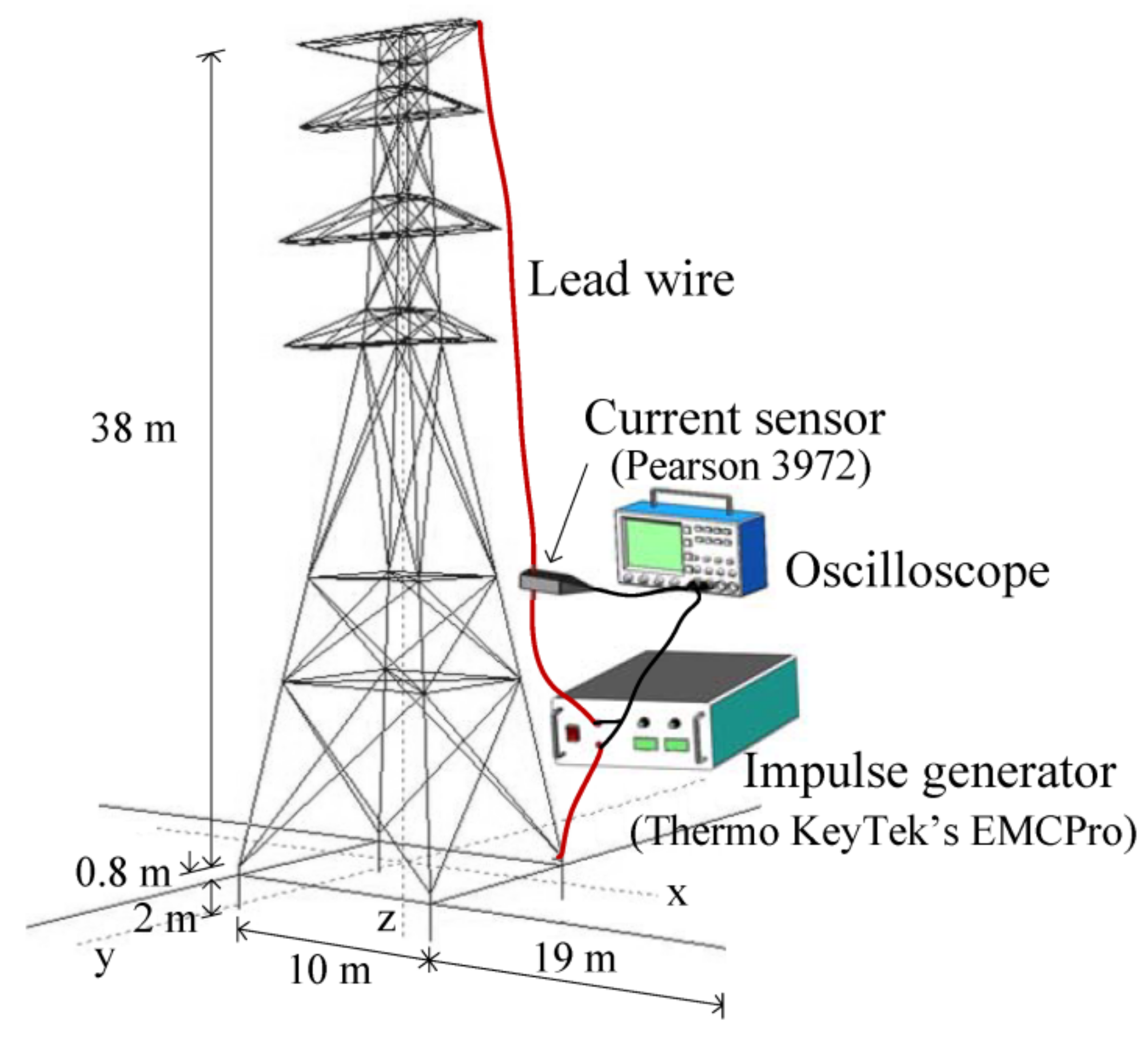
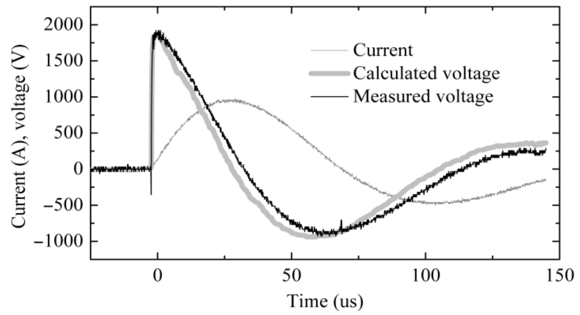
3.1. Field Test

In order to testify the model, a field test was conducted on a 220 kV transmission tower, as shown in Figure 4. The height of the tower is 38 m. The span of the legs is 10 m. The grounding device has four radial grounding electrodes, and each of them have a length of 19 m and a depth of 0.8 m. At each tower leg, there is an additional 2-m-long vertical grounding rod. The soil has a resistivity of 42 Ω m and a relative permittivity of 10. There was neither a phase conductor nor a ground wire on the tower.

Due to the load capacity constraints of the impulse generator, the equivalent impedance under test cannot be very large, and the lead wire cannot be too long. Thus, in our test, impulse current was just injected into the tower from its top through a lead wire, and was drawn back from one of the tower feet. Although this test can only obtain the transient performance of the tower body, the result can be used to testify the thin-wire model in this paper. Figure 5 shows the injected impulse current, the measured voltage, and the calculated voltage at the output of the impulse generator. In the calculation, the lead wire is also taken into account, which is a straight line connecting a top corner of the tower with one foot.

It can be seen from Figure 5 that the calculated and measured voltages are in good agreement. The rise time and the peak of the measured voltage are about 3.12 μs and 1902 V, while those of the calculated voltage are 2.98 μs and 1857 V. The errors are 4.45% and 2.37%, respectively. Therefore, the method in this paper is effective. Due to the load capacity constraints of the impulse generator, the front time of the impulse current is somewhat long. However, the front time of the voltage is very short. The voltage is almost proportional to the derivative of current over time. When the current begins to increase, the voltage reaches its peak quickly. When the current increase rate slows down, the voltage decreases. When the current decreases, the voltage becomes negative. Thus, it can be deduced that the whole tower and the lead wire can almost be regarded as an inductive load in this case, which is consistent with the existing conclusion that the tower can be regarded as an inductance [21].

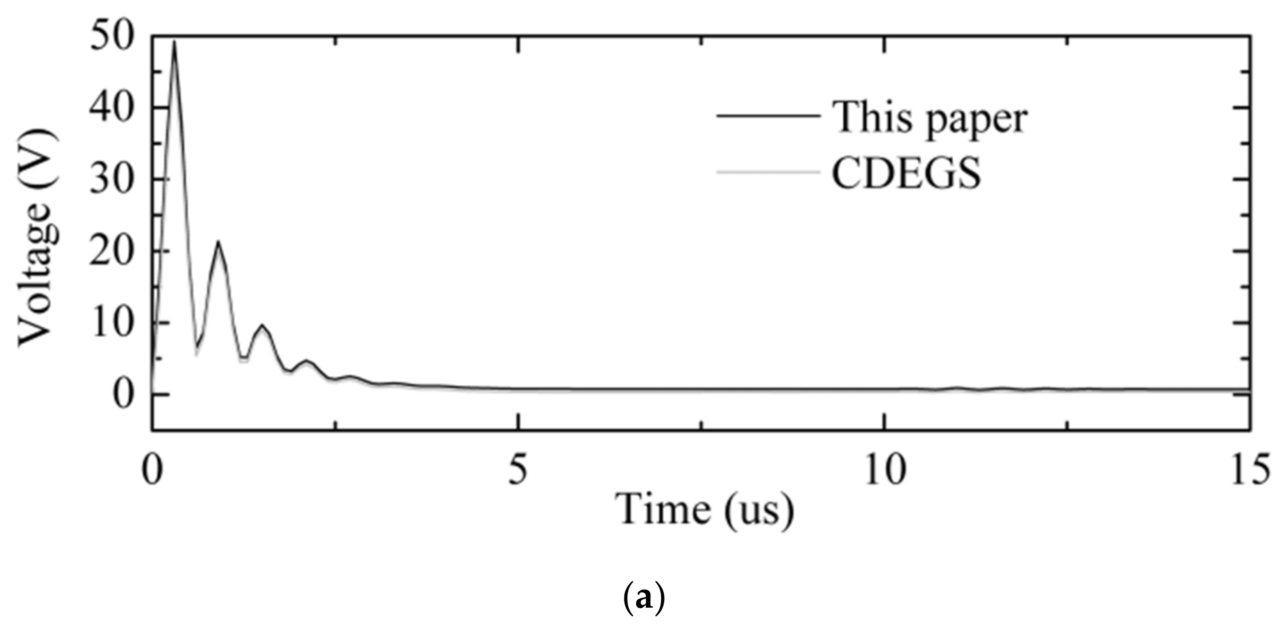
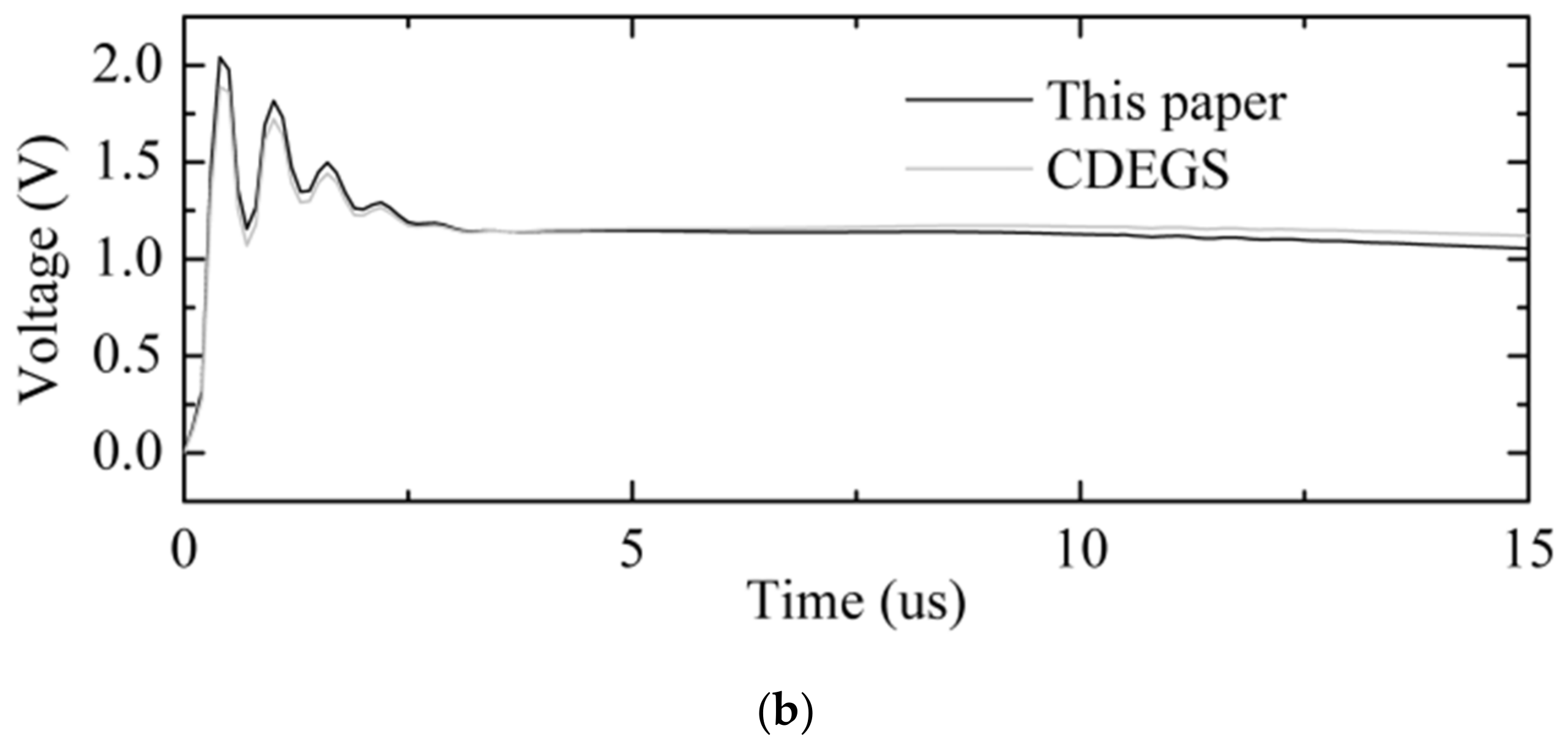
3.2. Comparison with Commercial Software

Since the above test can only verify the model for a tower, further verification should be provided when the tower and its grounding device are regarded as a whole. In this part, the response of the tower and its grounding device, as shown in Figure 4, is simulated with the help of a popular commercial software, CDEGS, which is developed based on MoM in the frequency domain [8]. In the calculation, a 2.6/50 μs lightning with a peak value of 1 A strikes the top of the tower directly, and there is no longer a lead wire. The result is compared with that obtained by the method in this paper, as shown in Figure 6. It can be seen that the two results are in good agreement. The error of the first voltage peak on the top of the tower is 1.71% and the error of corresponding time is 2.54%, while those at the foot of the tower are 8.89% and 5.14%, respectively. Therefore, the method in this paper is effective.

During the time when the lightning current increases very rapidly, the potential on the top of the tower is much greater than that at the tower feet. This is because the equivalent grounding resistance is very small compared with the equivalent impedance of the tower at this time [19]. When the variation of the lightning current becomes slow, the equivalent impedance of the tower reduces quickly. Then, the potential on the top of the tower drops noticeably, and the proportion of the potential at the tower feet begins to rise until the two potentials are almost equal.

At the beginning, the oscillation of the potentials is obvious. The oscillation frequency is closely related with the equivalent inductance and capacitance on the tower, which are also related to the tower height. Since the propagation velocity of the electromagnetic wave is the speed of light, the theoretical oscillation frequency can be estimated by f = 3 × 108/(4 h) Hz, where h is the tower height in meters. Therefore, if the tower height is 38 m, the theoretical oscillation frequency is 1.97 MHz. In this paper, due to the effect of various stray parameters, the oscillation frequency is about 1.8 MHz. The difference between the frequencies is acceptable, which also illustrates the effectiveness of the method.

4. Application

With the above method, the transient characteristics of a grounding grid with a lightning rod on the frame are calculated. Factors that affect the impulse grounding resistance and the ground potential distribution along the grounding grid are analyzed, such as the lightning stroke position, spacing between two adjacent grounding conductors, and the number of the grounded legs on the frame.

The grounding grid and the frame to be simulated are shown in Figure 7. The grid has an area of 200 × 200 m² and a burial depth of 0.8 m. The frame has a height of 25 m and three grounded legs. All of them are made of steel with a radius of 0.01 m, a resistivity of 1.75 × 10⁻⁷ Ω m, and a relative permeability of 636. In order to discharge the lighting current easily, there should usually be more grounding conductors near the lightning rod. Thus, as shown in Figure 7, near the grounded legs of the frame, the spacing between two adjacent grounding conductors is 5 m, while, in other places, the spacing is 20 m. The soil resistivity is 500 Ωm. A 2.6/50 μs lightning current with an amplitude of 1 A is injected into the grid. Because the nonlinear soil ionization is neglected in this paper, all responses are linear with the injected current.

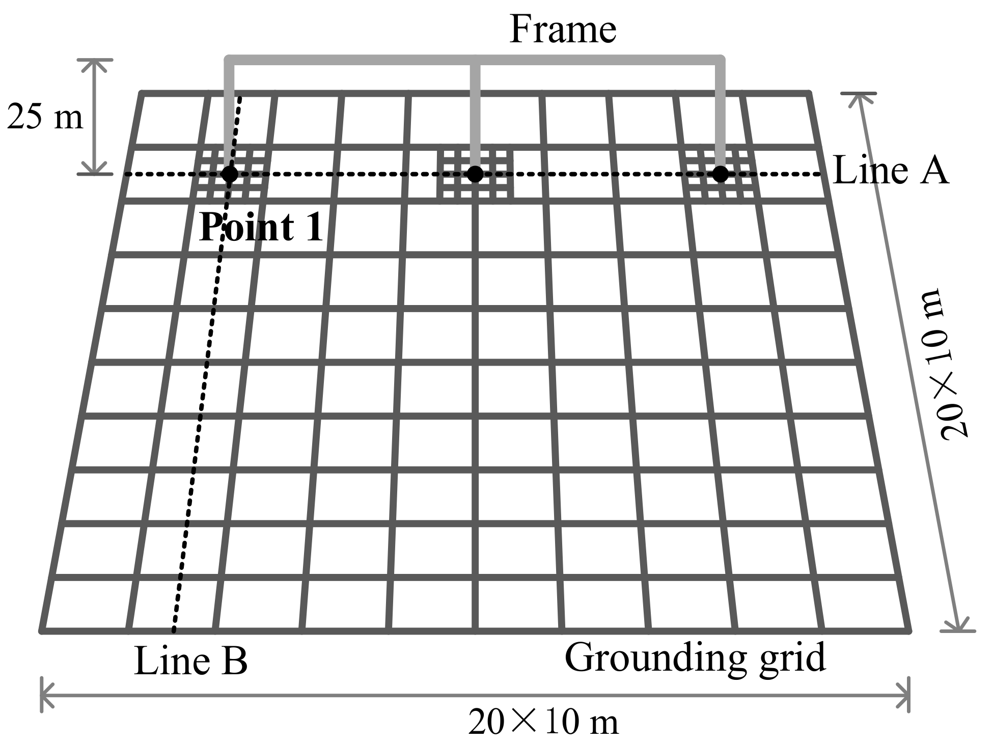
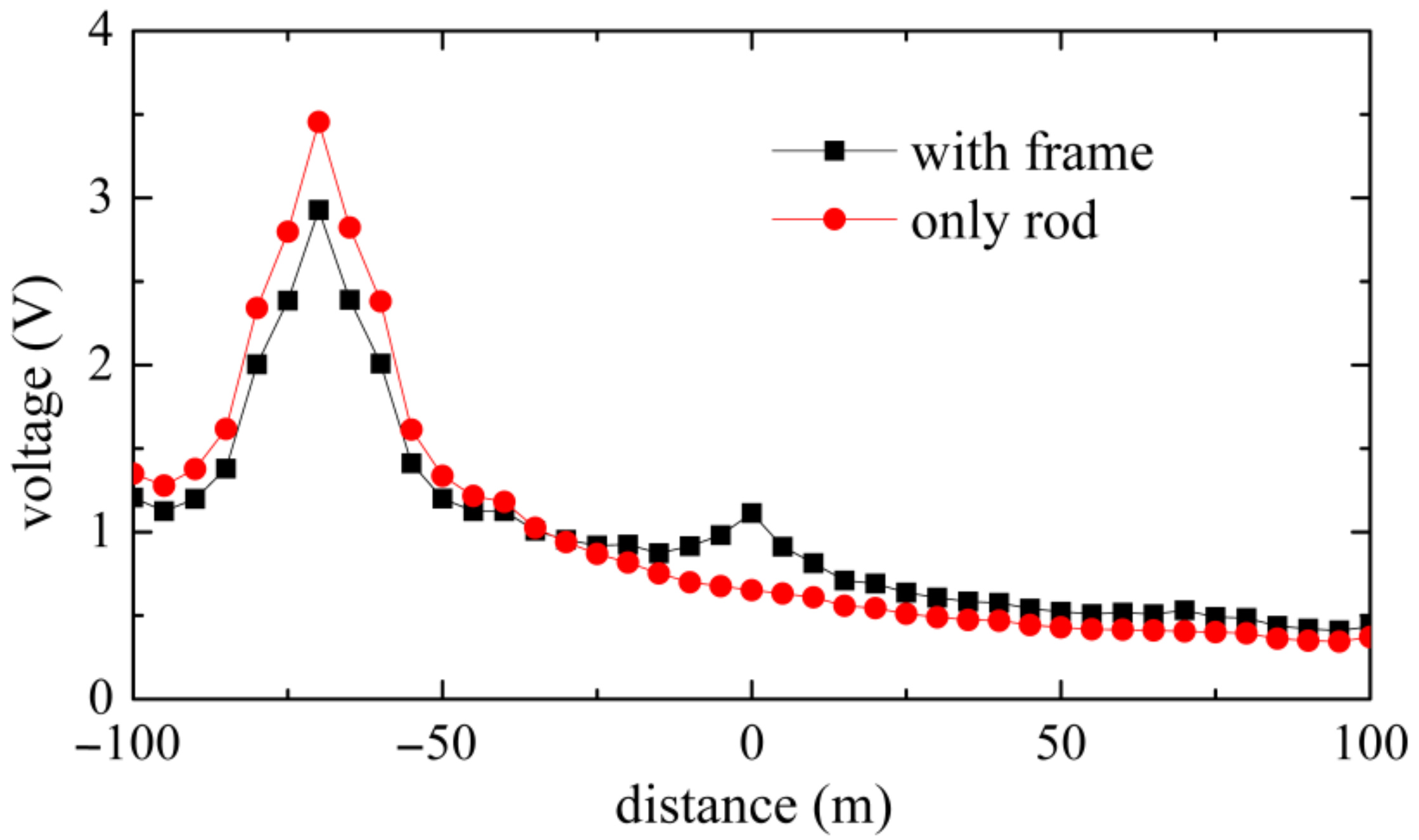
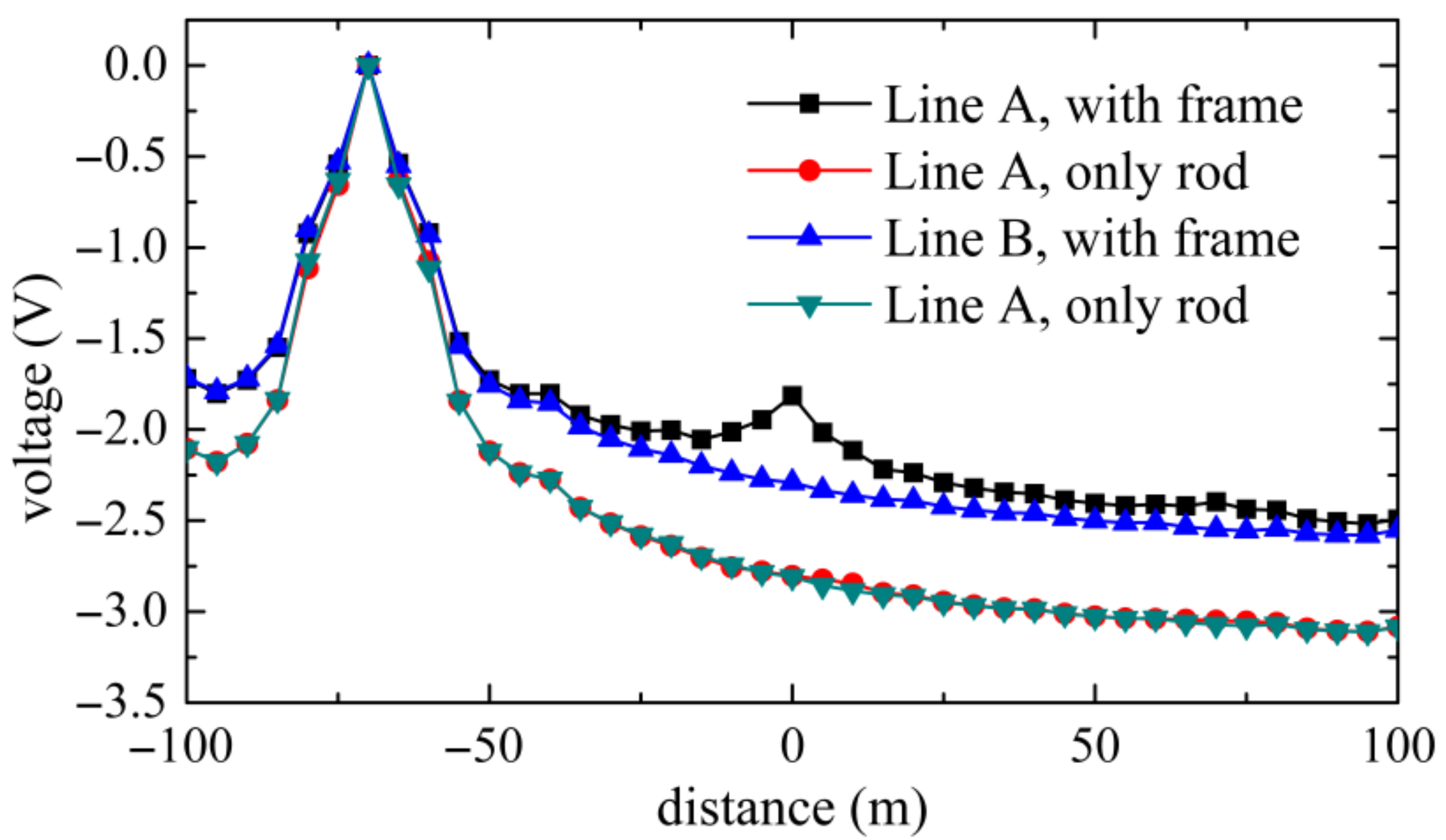
4.1. Potential Distribution along the Grounding Grid

When the lightning current is injected from the top of the leftmost side of the frame, the potential distributions along Line A and Line B that are shown in Figure 7, which have the same depth with the grounding grid, are calculated. At the same time, the potential distributions are also calculated when there is no frame but a lightning rod at point 1. Figure 8 and Figure 9 show the peak of the potential along the lines. Figure 10 shows the waveform of the transient potential at point 1.

It can be seen from the figures that:

• Near the lightning strike region, the maximal ground potential rise when the lightning strikes the frame is smaller than that when the lightning strikes a single lightning rod. In this paper, the gap between them is about 20%. Due to the shunting effect of the frame, part of the lightning current is injected into the grounding grid from other grounding points. On the other hand, the current shunted from the frame is just about 20%. Most of the current still enters the soil from the grounding electrode closest to the lightning strike. This may be due to the large inductance of the long frame.
• Moreover, due to the shunting effect of the frame, the ground potential rise at the grounding points of the frame far away from the lightning stroke region increases. However, the increase is limited.
• In the region far away from the grounding points of the frame, there is little difference between the results with and without the frame.
• The potential drops very rapidly near the lightning stroke point, while it becomes smooth in the faraway region. Due to the inductance along the grounding conductor, the lightning current tends to flow into the soil from the nearby region [22]. In this paper, the region where the potential drops fastest is that which is within 10 m from the current injection point. Thus, the equipment in the substation should be kept at least 10 m away from the grounding point for lightning.

The real threat to the safety of substations is the ground potential difference, not the ground potential rise. The ground potential difference between point 1 and the points on line A and line B is shown in Figure 11. It can be seen that the ground potential decrease rate within 25 m from point 1 is almost the same whether there is an independent lightning rod or a lightning rod on a frame. Therefore, even if there is a frame lightning rod, the same protective measures should be taken for the nearby facilities as those in the case of an independent lightning rod.

4.2. Effect of the Lightning Stroke Position

Due to the shunting effect of the frame, the potential difference will vary with the position of the lightning stroke. In this part, the effect of the lightning stroke position is simulated.

Since the potential decreases very rapidly near the current injection point, there is almost no equipment within 10 m. In this paper, the grounding grid is divided into two regions: that which is within 10 m of the current injection point is called the nearby region and that which is over 10 m away is called the faraway region. Both the maximal peak potential differences in the two regions are calculated as shown in

Table 1. Ground potential distribution under different lightning stroke positions.

Lightning Current Injection Positions	Leftmost	Middle
Maximal potential rise of grounding grid (V)	2.928	1.971
Maximal peak potential difference in nearby region (V)	1.218	0.772
Maximal peak potential difference in faraway region (V)	0.784	0.389
Maximal potential difference in the whole region (V)	1.538	0.807

.

The calculated results show that when the lightning current is injected from the lightning rod in the middle of the frame, all parameters are smaller than those when the lightning current is injected from one side. Obviously, this is because there are more shunt paths near the middle grounding point than others.

4.3. Effect of Spacing between Two Adjacent Grounding Conductors near the Current Injection Point

In order to easily discharge the lighting current, there should usually be more grounding conductors near the current injection point. In this paper, the effect of spacing between two adjacent grounding conductors in the nearby region is calculated when the lightning current is injected from the top of the leftmost side of the frame. The calculated results are shown in

Table 2. Ground potential distribution under different conductor densities.

Spacing of Nearby Conductors	2.5 m	5 m	10 m
Maximal potential rise of grounding grid (V)	2.795	2.928	3.331
Maximal peak potential difference in nearby region (V)	1.089	1.218	1.423
Maximal peak potential difference in faraway region (V)	0.794	0.784	0.777
Maximal potential difference in the whole region (V)	1.499	1.538	1.852

.

It shows that along with the increase in spacing of the nearby grounding conductors, all parameters (excluding the maximum potential difference in the faraway region) tend to increase. The maximal potential difference in faraway region stays almost constant and provides little contribution to the total ground potential increase. Thus, it is efficient to reduce the potential increase and the potential difference by increasing the density of the grounding conductors within 10 m of the grounding point.

4.4. Effect of the Number of Grounding Points along the Frame

It is clear that the number of grounding points affects the distribution of the lightning current to a great extent and further affects the distribution of the ground potential around the grounding grid. The paper analyzes the distribution when the frame has 2, 3 and 4 grounding points, respectively. The lightning current is injected from the top of the leftmost side of the frame. The calculated results are shown in

Table 3. Potential distribution of grounding grid with different numbers of grounding points.

Number of Ground Points	2	3	4
Maximal potential rise of grounding grid (V)	3.145	2.928	2.631
Maximal peak potential difference in nearby region (V)	1.441	1.218	1.126
Maximal peak potential difference in faraway region (V)	1.056	0.784	0.693
Maximal potential difference in the whole region (V)	2.006	1.538	1.427

.

As more grounding points means more paths for the lightning current, it shows that along with the increase in the number of grounding points, all parameters decrease gradually. The total lightning current diffusing into the ground from the grounding conductors close to the injection position is reduced; thus, the maximum potential difference of the area inside is reduced.

5. Conclusions

In this paper, a numerical model, in the time domain, is developed to simulate the lightning-caused electromagnetic transients on a frame and a grounding grid. The transient characteristics of the grounding grid, with lightning rods on the frame, are analyzed.

Although the frame causes the grounding potential increase to be evenly distributed, compared with the situation in which the lightning strikes a single lightning rod, the ground potential decrease rate near the main grounding point is almost the same because most of the current still enters the soil from the grounding electrode closest to the lightning strike. Therefore, even if there is a frame, the nearby facilities should take the same protective measures as in the case of an independent lightning rod. The ground conductors near the grounding point for lightning should be dense enough to reduce the potential gradient. The equipment should be kept at least 10 m away from the grounding point for lightning.

References

- IEEE Standards Board. IEEE Guide for Improving the Lightning Performance of Transmission Lines, 1st ed.; IEEE Standards Board: Piscataway, NJ, USA, 1997. [Google Scholar]
- Moselhy, A.H.; Abdel-Aziz, A.M.; Gilany, M.; Emam, A. Impact of first tower earthing resistance on fast front back-flashover in a 66 kV transmission system. Energies 2020, 13, 4663. [Google Scholar] [CrossRef]
- Dawalibi, F.; Xiong, W.; Ma, J. Transient performance of substation structures and associated grounding systems. IEEE Trans. Ind. Appl. 1995, 31, 520–527. [Google Scholar] [CrossRef]
- Brinner, T.R.; Durham, R.A. Transient-voltage aspects of grounding. IEEE Trans. Ind. Appl. 2010, 46, 1796–1804. [Google Scholar] [CrossRef]
- Chen, H.; Zhang, Y.; Du, Y.; Cheng, Q. Lightning propagation analysis on telecommunication towers above the perfect ground using full-wave time domain PEEC method. IEEE Trans. EMC 2019, 61, 697–704. [Google Scholar] [CrossRef]
- Alemi, M.R.; Sheshyekani, K. Wide-band modeling of tower-footing grounding systems for the evaluation of light-ning performance of transmission lines. IEEE Trans. EMC 2015, 57, 1627–1636. [Google Scholar]
- Grcev, L. Impulse Efficiency of Ground Electrodes. IEEE Trans. Power Deliv. 2008, 24, 441–451. [Google Scholar] [CrossRef] [Green Version]
- Lee, C.-H.; Chang, C.-N.; Jiang, J.-A. Evaluation of ground potential rises in a commercial building during a direct lightning stroke using CDEGS. IEEE Trans. Ind. Appl. 2015, 51, 4882–4888. [Google Scholar] [CrossRef]
- Ala, G.; Favuzza, S.; Francomano, E.; Giglia, G.; Zizzo, G. On the distribution of lightning current among interconnected grounding systems in medium voltage grids. Energies 2018, 11, 771. [Google Scholar] [CrossRef] [Green Version]
- Gholinezhad, J.; Shariatinasab, R. Time-domain modeling of tower-footing grounding systems based on impedance matrix. IEEE Trans. Power Deliv. 2018, 34, 910–918. [Google Scholar] [CrossRef]
- Zhang, B.; Wu, J.; He, J.; Zeng, R. Analysis of transient performance of grounding system considering soil ionization by time domain method. IEEE Trans. Magn. 2013, 49, 1837–1840. [Google Scholar] [CrossRef]
- Natsui, M.; Ametani, A.; Mahseredjian, J.; Sekioka, S.; Yamamoto, K. FDTD Analysis of Nearby Lightning Surges Flowing Into a Distribution Line via Groundings. IEEE Trans. Electromagn. Compat. 2019, 62, 144–154. [Google Scholar] [CrossRef]
- Viola, F.; Romano, P.; Miceli, R. Finite-difference time-domain simulation of towers cascade under lightning surge conditions. IEEE Trans. Ind. Appl. 2015, 51, 4917–4923. [Google Scholar] [CrossRef]
- Tatematsu, A.; Yamazaki, K.; Matsumoto, H. Lightning Surge analysis of a microwave relay station using the FDTD method. IEEE Trans. Electromagn. Compat. 2015, 57, 1616–1626. [Google Scholar] [CrossRef]
- Chen, H.; Du, Y.; Yuan, M.; Liu, Q. Analysis of the grounding for the substation under very fast transient using improved lossy thin-wire model for FDTD. IEEE Trans. EMC 2018, 60, 1833–1841. [Google Scholar] [CrossRef]
- Yutthagowith, P.; Ametani, A.; Nagaoka, N.; Baba, Y. Application of the partial element equivalent circuit method to analysis of transient potential rises in grounding systems. IEEE Trans. Electromagn. Compat. 2011, 53, 726–736. [Google Scholar] [CrossRef]
- Wang, S.; He, J.; Zhang, B.; Zeng, R. Time-domain simulation of small thin-wire structures above and buried in lossy ground using generalized modified mesh current method. IEEE Trans. Power Deliv. 2010, 26, 369–377. [Google Scholar] [CrossRef]
- Clavel, E.; Roudet, J.A.; Feuerharmel, H.; Luca, B.; Gouichiche, Z.; Joyeux, P. Benefits of the ground PEEC modeling approach—Example of a residential building struck by lightning. IEEE Trans. EMC 2019, 61, 1832–1840. [Google Scholar] [CrossRef] [Green Version]
- Chen, H.; Du, Y. Lightning grounding grid model considering both the frequency-dependent behavior and ionization phenomenon. IEEE Trans. Electromagn. Compat. 2018, 61, 157–165. [Google Scholar] [CrossRef]
- Van Bladel, J. Electromagnetic Field; Hemisphere Publishing, Co.: Washington, DC, USA; New York, NY, USA; London, UK, 1985. [Google Scholar]
- Conti, A.; Visacro, S.; Amilton, J. Revision, extension, and validation of jordan’s formula to calculate the surge impedance of vertical conductors. IEEE Trans. EMC 2006, 48, 530–536. [Google Scholar] [CrossRef]
- He, J.; Gao, Y.; Zeng, R.; Zou, J.; Liang, X.; Zhang, B.; Lee, J.; Chang, S. Effective length of counterpoise wire under lightning current. IEEE Trans. Power Deliv. 2005, 20, 1585–1591. [Google Scholar] [CrossRef]