Stationarity in the Prices of Energy Commodities. A Nonparametric Approach

Abstract

In this paper, we address the classical problem of testing for stationarity in the prices of energy-related commodities. A panel of fourteen time series of monthly prices is analyzed for the 1980–2020 period. Nine of the series are classical nonrenewable, GHG-emissions-intensive resources (coal, crude oil, natural gas), whereas the remaining, low-emission group includes both uranium and four commodities employed in biofuels (rapeseed, palm, and soybean oils, and ethanol). A nonparametric, bootstrap-based stationarity testing framework is employed. The main advantage of this procedure is its asymptotically model-free nature, being less sensitive than parametric tests to the risks of misspecification and detection of spurious unit roots, although it has the potential limitation of typically requiring larger samples than mainstream tools. Results suggest that most of the series analyzed may be trend stationary. The only exception would be crude oil, where different conclusions are obtained depending on whether a seasonal correction is applied or not.

1. Introduction

Stationarity/unit-root analysis is a relevant topic in a great many fields, including climate change studies and commodities modeling. As well known, the goal is to distinguish time series that may be properly modeled as stochastic processes having stationary oscillations around their (usually time-varying) means from those with characteristics more closely resembling those of integrated random processes.

That distinction has practical relevance in many areas including assessment of the validity of theories, policy design and analysis (as integrated processes typically require more proactive policies to correct for the effect of shocks, these being less necessary in trend-stationary processes, where their natural inertia leads them to mean-revert), and econometric estimation and subsequent application of models to forecasting (where the optimal predictors clearly differ in stationary and integrated cases) and decision making. For instance, in the specific area of energy, Pindyck [1], among others, stressed the relevance (for both long-run forecasting and firms making investment decisions) of knowing the stochastic properties of energy prices, whereas Felder [2] focuses on the importance of long-term fuel price forecasts to both determine correct choices of fuel mix and evaluate fuel diversification strategies.

From the standpoint of the application of stationarity for the assessment of theories validity, a widely discussed framework is Hotelling’s model, which predicts that in a world of certainty, non-renewable resource prices would be trend stationary. The classical monograph by Slade [3] was one of the first attempts to evaluate Hotelling’s model through the analysis of the time series properties of natural resource prices. Subsequent papers (e.g., Presno et al. [4], among many others) extended the analysis.

In the field of energy, many research papers have employed stationarity testing with a view to investigating the efficient market hypothesis. For instance, Lee and Lee [5] found stationarity around a broken trend, thus concluding that energy prices do not show efficiency in their markets. Other papers in the field (e.g., Maslyuk and Smyth [6]) have focused on various non-renewables energy series, with their analyses relying on a wide variety of techniques. Unit-root/stationarity testing is also being employed to detect potential bubbles in asset prices (e.g., Perifanis [7] and Floros and Galyfianakis [8] have studied the case of crude oil prices).

Unit root and stationarity tests have also been applied in relation to assessing the Prebisch–Singer hypothesis, which originally poses that the relative prices of primary commodities (in terms of manufactures) are stationary around a downward trend. Subsequent papers (e.g., Sapsford [9], among others) have analyzed this hypothesis.

The distinction between stationary and integrated processes also has relevance from the perspective of stabilization policies. Regarding this, Reinhart and Wickham [10] highlighted the greater effectivity of hedging and stabilization strategies when commodity prices are stationary, whereas structural policies would be required when they are affected by temporary but widespread, highly persistent shocks.

In the case of commodities, large price variations (as caused by demand and supply dynamics) are frequently observed in the markets. Although stockholding certainly brings about some price smoothing, prices often jump sharply. Those moves are particularly relevant in the crude oil markets, since they are affected by natural disasters, geopolitical or unforeseen events, and strategic actions that may lead to unexpected, large changes in prices. The relevance of these discontinuities for modeling oil prices has been studied, among others, by Askari and Krichene [11].

Knowledge of the statistical properties of energy commodity prices also has evident interest from the standpoint of trading (e.g., Knittel and Pindyck [12]) and investing, both in commodities and in the stocks of commodity-related companies, as well as in price volatility modeling (e.g., Narayan and Narayan [13]), and also from the perspective of constructing suitable price indexes, specifically oriented to environmental, energy or financial goals (e.g., Tang and Xiong [14]).

In this paper, we revisit the problem of stationarity testing in energy-related commodities. A panel of fourteen time series of monthly prices is analyzed for the 1980–2020 period. Nine of the series correspond to nonrenewable, emissions-intensive resources (coal, crude oil, natural gas). The rest of the series (‘low-emission’ group) includes uranium and four commodities employed in biofuels.

Nuclear energy, beyond its potential risks, is increasingly considered among the sustainable, yet not renewable, sources. As for biofuels, they are renewable and considered as low-emission, although many of them are not exchanged in official markets. We have focused on four of the most economically relevant cases, namely ethanol, and soybean, rapeseed, and palm oils. These are not ‘pure’ energy commodities, as they are regularly employed in many other areas (including the chemical and food industries), so their price patterns may be somewhat different from other energy-related commodities.

The first novelty of the paper is the analysis, in an integrated fashion, of a group of energy-related commodities that includes both classical ones (more exhaustively studied in the literature on non-renewable resources) and low-emission resources including uranium and biofuels that are less frequently analyzed.

A second contribution stems from the methodology employed, namely a nonparametric panel stationarity test recently proposed by Presno et al. [15] with a view to addressing the problems of low power and sensitivity to misspecification that affect mainstream, parametric stationarity/unit-root tests. The nonparametric approach to stationarity testing is asymptotically model-free, so the risk of misspecification of the deterministic mean function of each series (that typically induces detection of spurious unit roots) should be greatly reduced, with more robust testing results being expected in those cases where there exist reasonable doubts on the correctness of the parametric model specifications employed. This situation may well be prevalent in the case of the time series of commodity prices, that usually exhibit very complex time patterns. A potential limitation of this approach stems from the fact that nonparametric estimation and testing devices typically require larger samples than their conventional parametric counterparts, which may reduce their power (and advice against their use) in those applications where only small samples are available.

The analysis is first carried out for the raw, nominal price series, and then sequentially for the same series deflated by the US Consumer Price Index, and for the de-seasonalized and deflated series. This way, we can assess the potential effects of the various transforms on the testing process and its conclusions. The panel study is complemented with a study of stationarity for the individual series.

The remainder of this paper is organized as follows. Section 2 includes a review of the literature in the field. Section 3 briefly outlines the methodology employed and presents the time series to be analyzed. Section 4 summarizes the main results of the analysis. Section 5 includes a discussion and some comments on their implications for environmental and energy policies. Section 6 concludes with some final remarks and potential research avenues.

2. Literature Review

There now exists abundant literature analyzing price stationarity for nonrenewable, emissions-intensive resources like coal, oil, and natural gas, with mixed results depending on the various markets, observation frequencies, and time periods considered (e.g., Alvarez-Ramirez et al. [16]). Certainly, coal, oil, and natural gas still account for more than 80% of global energy consumption (85% according to Kahouli [17]), being responsible for a significant share of greenhouse gas (GHG) emissions. With climate change as a backdrop, attention has focused on renewable energies, which are progressively reaching greater shares in the energy mix of countries. Moreover, since renewable energy sources are still unable to supply relevant volumes of baseload power, the debate has also revived on nuclear energy as an alternative to carbon-emitting sources and its role in energy security.

As pointed out by Baffes [18], energy prices and the food markets are also connected, with high-energy prices increasing the cost of producing food commodities and encouraging policies to produce biofuels from food crops (Kapusuzoglu and Karacaer Ulusoy [19]). A few studies have focused on analyzing stationarity in the prices of some commodities currently employed as biofuels. Most papers have focused on crude palm oil. This is the leading (most heavily consumed and traded) commodity in the edible oil market, with a production that nearly quintupled between years 1990 and 2013. Palm oil was one of the eighteen primary commodity price series included in the classical study by Grilli and Yang [20] and has been subsequently studied in many papers. More recently, Lean and Smyth [21], who analyzed palm oil spot and futures markets by employing a GARCH unit root test with structural breaks, concluded that a large percentage of the palm oil series they analyzed are stationary, with only a weak evidence of efficiency being found in that market. Efficiency in the palm oil market has also been addressed by Liu [22], and more recently by Snaith et al. [23], whose results suggested an efficiency skew in the market, and Lee et al. [24], who concluded that the crude palm oil market is more efficient than that of the West Texas Intermediate crude oil. Chen et al. [25], employing unit root Augmented Dickey-Fuller (ADF) testing with no changes allowed for, found significant evidence of unit roots in both palm and soybean oils. These two oils were also analyzed by Cashin et al. [26] in their extensive study on persistence of the shocks in commodity prices.

As for ethanol, it has been studied by Chang et al. [27], who analyzed the volatility spillovers in both spot and futures returns of that commodity (and of two related—namely corn and sugarcane—products), concluding stationarity. A few papers have also tested the unit root hypothesis in the case of uranium. Kahouli [28], using ADF and Phillips–Perron tests in no-change models (integrated in a more complex vector autoregressive scheme), detected unit roots in the price of that commodity. The same conclusion was reached by Chen et al. [25], whose analysis relied on panel unit root testing.

From the standpoint of methodology, as commented above, we rely on the nonparametric, panel stationarity testing framework. This approach aims at simultaneously addressing two of the problems (namely low power and lack of robustness to misspecification of the deterministic component of the process) that plague mainstream unit-root and stationarity testing. The low power problem has previously been tackled in literature by producing panel tests that extend unit-root and stationarity testing to the case of vector processes. Some classical contributions in the field include Carrion et al. [29] and Pesaran [30], among many others. The problem of sensitivity to misspecification, that in the case of stationarity testing typically results in detection of spurious unit roots in the series, was analyzed by Landajo and Presno [31], who proposed a nonparametric, limiting standard normal extension of the classical stationarity test of Kwiatkowski et al. [32] (hereafter KPSS), that asymptotically avoids the effects of misspecification and delivers a correct-sized, consistent test. More recently, Presno et al. [15] combined both approaches in a so-called nonparametric panel stationarity test, which was implemented through bootstrapping.

3. Materials and Methods

3.1. Methodology

The prices of commodities are assumed to come from a panel of N time series ${\mathit{y}}_t=\left(y_{1,t},\dots , y_{N,t}\right)$ generated by the following process:

$$y_{i,t}={\mu }_{i,t}+{\theta }_i^{*}\left(\raisebox{1ex}{$t$}\!\left/ \!\raisebox{-1ex}{$T$}\right.\right)+{\epsilon }_{i,t},$$

(1)

$${\mu }_{i,t}={\mu }_{i,t-1}+u_{i,t} ; t=1,\dots ,T; i=1, 2, \dots , N$$

where θi*:[0,1] → ℝ is the the deterministic trend (or more generally, the mean) function of the i-th component of the panel and ${\mathbf{\epsilon }}_t=\left({\epsilon }_{1,t}, \dots , {\epsilon }_{N,t}\right)$ is a zero-mean random vector process (with both serial dependence and cross-correlation being allowed). It is also assumed that, for any i = 1, …, N, the processes {ε_i,t, t = 1, 2, …} and {u_i,t, t = 1, 2, …} are independent of each other, with zero means and respective (finite) variances $E({\epsilon }_{i,t}^2)={\sigma }_{i,\epsilon }^2>0$ and $E(u_{i,t}^2)={\sigma }_{i,u}^2 \ge 0$; {μ_i,t} starts with μ_i,0, which is assumed to be zero.

Stationarity testing can be carried out both separately for each series and jointly for the whole panel. The panel testing problem is as follows:

$$H_0: q_i\equiv \frac{{\sigma }_{i,u}^2}{{\sigma }_{i,\epsilon }^2}=0 \mathrm{for} i =1, \dots , N, \mathrm{versus} H_1:{\displaystyle \sum }_{i=1}^N{q}_i>0$$

(2)

In the above setting, the variance of $u_{i,t}$ is zero under the null hypothesis, so ${\mu }_{i,t}=0$ (with probability 1, for each $t=1,2,\dots , i=1,\dots ,N$) in that case and the model for each series in the panel reduces to $y_{i,t}={\theta }_i^{*}\left(\raisebox{1ex}{$t$}\!\left/ \!\raisebox{-1ex}{$T$}\right.\right)+{\epsilon }_{i,t}$ (i.e., all the series exhibit stationary oscillations around their deterministic means). Under the alternative, the variance of $u_{i,t}$ is positive for at least one $i=1,\dots ,N$, so we have ${\mu }_{i,t}=u_{i,1}+\dots +u_{i,t}$, which is an integrated process (e.g., a random walk) that is nested in $y_{i,t}={\mu }_{i,t}+{\theta }_i^{*}\left(\raisebox{1ex}{$t$}\!\left/ \!\raisebox{-1ex}{$T$}\right.\right)+{\epsilon }_{i,t}$, and therefore at least one (though not necessarily all) of the components of the panel has a unit root. Separate stationarity testing for any individual series may be carried out along the same lines.

In the nonparametric extension of classical KPSS stationarity testing proposed by Landajo and Presno [31], the trend function $-{\theta }_i^{*}\left(\raisebox{1ex}{$t$}\!\left/ \!\raisebox{-1ex}{$T$}\right.\right)-$ of series $y_{i,t}$ is first estimated nonparametrically, through an OLS regression of $y_{i,t}$ on the elements of a cosine basis, so the following estimator is obtained:

$${\widehat{\theta }}_i\left(\raisebox{1ex}{$t$}\!\left/ \!\raisebox{-1ex}{$T$}\right.\right)={\widehat{\beta }}_{i,o}+{\displaystyle \sum }_{j=1}^{m_T}{\widehat{\beta }}_{i,j}\cos \left(j\pi t/T\right)$$

(3)

Nonparametric estimation of the trend function avoids the problems associated with the need of a priori specifying a correct functional form for the deterministic component of the model, so the misspecification risk—that tends to result in spurious unit roots being detected—is (asymptotically) circumvented. To obtain a consistent test, model complexity ($m_T)$ in Equation (3) above must increase along with sample size (T) at a suitably restricted rate. Here, we shall use the same deterministic rule as Landajo and Presno [31], namely, $m_T=\left[4T^{1/5}\right]$, with $[\cdot ]$ being the integer part function.

Then the raw stationarity test statistic for time series $y_{i,t}$, namely ${\widehat{S}}_{i,T}$, is readily computed from the residuals of the above cosine regression, namely:

$${\widehat{S}}_{i,T}={\frac{{{\displaystyle \sum }}_{t=1}^T\left({{\displaystyle \sum }}_{k=1}^t{\widehat{\epsilon }}_{i,k}\right)}{{\widehat{\sigma }}_i^2{T}^2}}^2$$

(4)

with ${\widehat{\epsilon }}_{i,k}=y_{i,k}-{\widehat{\theta }}_i\left(\raisebox{1ex}{$k$}\!\left/ \!\raisebox{-1ex}{$T$}\right.\right)$, $k=1,\dots ,T$, and ${\widehat{\sigma }}_i^2$ being a suitable estimator for the long run variance of $y_{i,t}$. The standardized stationarity test statistic for series $y_{i,t}$ is calculated as:

$${\widehat{Z}}_{i,T}=\frac{{\widehat{S}}_{i,T}-{\mu }_{m_T}}{s_{m_T}}$$

(5)

with ${\mu }_{m_T}$ and $s_{m_T}$ being suitable standardization factors (namely, ${\mu }_{m_T}={\displaystyle \sum }_{j=m_T+1}^{\infty }{\left(j\pi \right)}^{-2}$,$s_{m_T}^2=2{\displaystyle \sum }_{j=m_T+1}^{\infty }{\left(j\pi \right)}^{-4}$, and $s_{m_T}=+\sqrt{s_{m_T}^2}$). The limiting null distribution of ${\widehat{Z}}_{i,T}$ is standard normal, whereas it diverges in probability to ∞ under the unit root alternative, so a consistent test is obtained.

In the panel setting, Presno et al. [15] relied on the usual procedure of averaging the individual test statistics, so the null of joint stationarity in Equation (2) is tested by employing the following nonparametric panel stationarity (NPS) test statistic:

$${\overline{Z}}_T=\frac{{{\displaystyle \sum }}_{i=1}^N{\widehat{Z}}_{i,T}}{N}$$

(6)

The limiting null distribution of ${\overline{Z}}_T$ is unknown, so they proposed a feasible, bootstrap-based implementation. We shall also rely on the bootstrap to carry out both the individual and panel stationarity tests (the algorithms and further technical details may be found in Presno et al. [15]).

3.2. The Dataset

As commented above, the time series to be analyzed are monthly prices of fourteen energy-related commodities. Details are provided in

Table 1. The commodity prices analyzed.

Commodity Group	Series
Coal	US Producer Price Index by Commodity: Fuels and Related Products and Power: Coal. *
	Coal, Australian thermal coal, 12,000-btu/pound, less than 1% sulfur, 14% ash, FOB Newcastle/Port Kembla, US$ per metric ton. **
	Coal, South African export price, US$ per metric ton. **
Oil	Crude Oil (petroleum), West Texas Intermediate 40 API, Midland Texas, US$ per barrel. **
	Crude Oil (petroleum), Dated Brent, light blend 38 API, fob U.K., US$ per barrel. **
	Crude Oil (petroleum), Dubai Fateh 32 API, US$ per barrel. **
Natural gas	Natural Gas spot price at the Henry Hub terminal in Louisiana, US$ per Million Metric British Thermal Unit. **
	Netherlands TTF Natural Gas Forward Day Ahead, US$ per Million Metric British Thermal Unit. **
	Indonesian Liquefied Natural Gas in Japan, US$ per Million Metric British Thermal Unit. **
Uranium	Uranium, NUEXCO, Restricted Price, Nuexco exchange spot, US$ per pound. **
Biofuels	Producer Price Index by Commodity: Chemicals and Allied Products: Ethanol. (Some parts of the ethanol series had to be reconstructed by linear interpolation in those periods—namely 1:1989–7:1991; 6:1995–7:2001; 12:2003–1:2005—when calculation of the series was discontinued.)
	Soybean Oil, Chicago Soybean Oil Futures (first contract forward) exchange approved grades, US$ per metric ton. **
	Rapeseed oil, crude, fob Rotterdam, US$ per metric ton. **
	Palm oil, Malaysia Palm Oil Futures (first contract forward) 4–5 percent FFA, US$ per metric ton. **

Sources: *: U.S. Bureau of Labor Statistics, retrieved from FRED, Federal Reserve Bank of St. Louis. **: International Monetary Fund.

below.

As for uranium, a recent report by the International Energy Agency [33] underlines the role of nuclear power as the second-largest source of low-carbon electricity today, with 452 operating reactors providing 10% of global electricity supply in 2018. The same report states that “achieving the clean energy transition with less nuclear power is possible but would require an extraordinary effort”. Although the use of nuclear energy is polemical, especially in areas like North America and the European Union where its share in the energy mix may be progressively decreasing in years to come (with many reactors scheduled to be retired around 2030 and beyond), new nuclear capacity is currently being added in other regions, mainly in emerging economies like China, India, and Russia, but also in South Korea and the United Arab Emirates, among others.

Cole [34] stressed the potential for distortionary effects on uranium markets as a consequence of factors such as a strong regulatory framework, competition from unconventional secondary supply, and the idiosyncratic nature of that commodity. He detects both similarities with other commodities (sharing their cyclical behavior) and simultaneous evidence of “a strange behavior”, with sharp booms much shorter than the average of commodities and deep slumps that are the longest of all commodities. Uranium price had spectacular rises in the early 1970s and at the beginning of this century. Testing for bivariate cointegration between uranium and its energy substitutes, Cole [34] detected a weak cointegration with crude oil, but not with coal and natural gas, whereas Kahouli [17] found that coal is the only fuel positively correlated with uranium price. A recent study by Pedregal [35], employing a wide range of predictive tools, also underlined the difficulty of forecasting uranium prices, with sophisticated linear/nonlinear approaches typically beaten off by naïve predictors.

Biofuels are high priority in regions like the European Union, Brazil, and the United States, because of both their focus in reducing GHG emissions and concerns on excessive dependence on oil imports. In the case of Europe, Directive (EU) 2018/2001 (known as RED II and entered into force on 1 January 2021) sets (among many other goals) binding targets for the use of advanced, non-food-based biofuels to 3.5% by 2030, and a blending cap of 1.7% for advanced biofuels produced with waste fats and oils. Indeed, advanced biofuels will be double counted in relation to both the above 3.5% target and the 14% target for renewable energy use in transport by 2030. RED II also introduced sustainability criteria for biomass and expanded sustainability criteria in the case of liquid biofuels. The four biofuels included in our analysis may all be regarded as first generation, rather than advanced biofuels, but organized markets and time series of historical prices were only available for the former.

Ethanol is a renewable fuel made from biomass (mainly corn, cane sugar, and sugar beet). It now amounts to about 80% of the global production of liquid biofuels. The United States is the world leader in production (54% of world output in 2019), consumption, and export of ethanol, followed by Brazil (with a 30% share in world production in the same year). Nowadays more than 98% of U.S. gasoline contains ethanol (typically 10% ethanol, 90% gasoline) to oxygenate the fuel, which reduces air pollution. It is also available as “flex fuel” that can be used in flexible fuel vehicles which can operate on any blend of gasoline and ethanol up to 83%.

Raw vegetable oils like soybean, corn, rapeseed/canola, and palm are employed to produce biodiesel that may be used either unblended (for engines operating on pure biofuels) or combined with refined petroleum (in regular diesel engines). Biodiesel production is less concentrated than ethanol. The EU has remained the center of global biodiesel production. Soybean oil is the main feedstock (followed at a considerable distance by recycled feeds and corn and canola oils) for biodiesel production in the United States. Biodiesel production represents an increasing share (currently accounting for about 30%) of domestic soybean oil disposition in that country. In the European Union—where biofuel production has doubled since 2008, with Germany being the leading producer—around 14 million metric tons of oil equivalent biodiesel are consumed each year. European countries currently use rapeseed, palm, and sunflower oils as their main feedstock for biodiesel production. According to the 2019 Renewable Energy Progress report (COM/2019/225 final), around 70% of EU’s rapeseed oil is employed in biodiesel production, with roughly a 45% share in EU biodiesel in year 2016. Palm oil (not including related products) amounted to 20% in that year, after steadily increasing in the last decade, pushed up by development of hydrotreated vegetable oil (HVO) capacities, although the weight of palm oil may be decreasing in years to come as a consequence of Directive RED II (2018/2001/EC) compromise for stabilization of biodiesel and the plans to eliminate palm oil by year 2030 (Dusser [36]). Palm oil is also employed as feedstock for biodiesel production in South-East Asia (mainly Malaysia and Indonesia, which also supply about 85% of global palm oil, mostly for food and cosmetic uses).

The study period we consider is relatively recent, with much larger data sets being available for some of the series analyzed (e.g., US coal). Our choice of a shorter period reduces the heterogeneity problems associated with very long time series (e.g., price series are available since the 1960s in the case of ethanol, whereas its extensive use as a fuel is relatively recent, which potentially creates noncomparability/heterogeneity problems when analyzing the complete time series as a fuel price).

For some commodities (coal, natural gas, oil), we analyze several prices corresponding to different geographic origins. In principle, the law of one price implies that in the absence of friction, given the possibility of arbitrage, prices would be roughly the same in the various markets corresponding to each commodity, so qualitatively similar results should be expected when analyzing stationarity in the various markets corresponding to the same commodity. It is also reasonable to expect parallel results for the various biofuels, given that in most cases they are close substitutes for each other.

The commodity series were first de-seasonalized by employing the X-12-ARIMA monthly seasonal adjustment method by the U.S. Census Bureau. Then, they were deflated by using the US Consumer Price Index (US CPI). Although all deflators have limitations, this is a common choice (e.g., Jacks and Stuermer [37]). Other possibilities would include using producer price indexes (PPI) (e.g., Enders and Holt [38]) or the Manufacturing Unit Value (MUV) index (e.g., Erten and Ocampo [39]). The results for the raw (nominal) prices are also included for the sake of comparison.

4. Results

Table 2. Panel nonparametric stationarity testing results (B = 10,000 bootstrap resamples).

Product\Treatment	RAW	US-CPI-Deflated	Deseasonalized, Deflated
	Obs. NPS Test Statistic (p-Value)	Obs. NPS Test Statistic (p-Value)	Obs. NPS Test Statistic (p-Value)
Coal (period: 1990:01–2020:11)	−1.171 (p = 0.990)	−1.128 (p = 0.987)	−0.853 (p = 0.999)
Crude oil (period: 1980:01–2020:11)	2.761 (p = 0.068)	2.725 (p = 0.061)	1.347 (p = 0.205)
Natural gas (period: 992:01–2020-11)	1.593 (p = 0.612)	1.623 (p = 0.585)	−1.768 (p = 0.992)
Biofuels (period: 980:01–2020-11)	−1.263 (p = 0.989)	−1.328 (p = 0.992)	−2.168 (p = 0.999)

and

Table 3. Individual nonparametric stationarity testing results (B = 10,000 bootstrap resamples).

Product\Treatment	RAW	US-CPI-Deflated	Deseasonalized, Deflated
	Obs. NPS Test Statistic (p-Value)	Obs. NPS Test Statistic (p-Value)	Obs. NPS Test Statistic (p-Value)
Australian coal (period 1980:01–2020-11)	−1.293 (p = 0.988)	−1.365 (p = 0.993)	−0.992 (p = 0.984)
South African coal (period 1990:01–2020-11)	−0.643 (p = 0.963)	−0.696 (p = 0.966)	0.207 (p = 0.941)
U.S. coal (period: 1980:01–2020:11)	−1.213 (p = 0.962)	−1.067 (p = 0.948)	−1.544 (p = 0.985)
Brent crude oil (period: 1980:01–2020:11)	1.341 (p = 0.090)	1.321 (p = 0.095)	0.562 (p = 0.264)
Dubai crude oil (period: 1980:01–2020:11)	1.961 (p = 0.040)	1.937 (p = 0.044)	0.886 (p = 0.191)
West Texas crude oil (period: 1980:01–2020:11)	1.481 (p = 0.082)	1.462 (p = 0.077)	0.885 (p = 0.175)
Indonesian natural gas (period: 1992:01–2020:11)	2.688 (p = 0.131)	2.690 (p = 0.128)	−1.723 (p = 0.985)
Netherlands natural gas (period: 1985:01–2020:11)	−0.763 (p = 0.897)	−0.744 (p = 0.899)	−2.207 (p = 0.999)
Henry Hubb natural gas (period: 1991:01–2020:11)	−0.256 (p = 0.644)	−0.231 (p = 0.612)	−1.299 (p = 0.914)
Uranium (period: 1980:01–2020:11)	−1.689 (p = 0.974)	−0.994 (p = 0.850)	−1.659 (p = 0.967)
Ethanol (period: 1980:01–2020:11)	0.562 (p = 0.125)	0.633 (p = 0.127)	0.610 (p = 0.118)
Soybean oil (period: 1980:01–2020:11)	−0.170 (p = 0.666)	−0.098 (p = 0.617)	−0.532 (p = 0.809)
Rapeseed oil (period: 1980:01–2020:11)	−1.014 (p = 0.751)	−0.881 (p = 0.682)	−1.765 (p = 0.998)
Palm oil (period: 1980:01–2020:11)	−1.813 (p = 1)	−1.795 (p = 1)	−2.127 (p = 1)

below show the results of stationarity testing. All the series are analyzed in logarithmic scale. Table 2 includes the results at the panel level, with the panels being coal (USA, Australian, South African), natural gas (Henry Hubb, Netherlands, Indonesia), oil (West Texas, Brent, Dubai), and biofuels (ethanol; soybean, rapeseed, and palm oils). Uranium is treated as a single-element panel (results in Table 3). With a view to controlling for potentially adverse effects of the various kinds of filtering applied to the data, we report the results in three different settings, namely for (i) the nominal price series, (ii) the series deflated with the US CPI, and (iii) the series previously de-seasonalized (by employing Census X-12-ARIMA procedure) and then deflated with the US CPI. This allows us to separate the potential effects of the various treatments. Ideally, the deflated series should be closer to a series of ‘real’ prices, with the effect of inflation (i.e., dollar depreciation) factored out (admittedly, in an imperfect fashion). De-seasonalizing the series aims at filtering out seasonal effects. For commodities, the presence of seasonality in returns would clearly be in a conflict with the notion of market efficiency, although many papers (e.g., Fama and French [40]) point out that those effects may actually exist.

Results of the nonparametric panel stationarity tests in Table 2 indicate that, with the only exception of crude oil, stationarity fails to be rejected (with very high p-values) in all cases, regardless of the commodity group analyzed, the nature (renewable, non-renewable), and the treatment applied to the series. The evidence is more ambiguous in the oil panel, as stationarity is weakly rejected (with p-values of 6–7%) in the cases of the raw and deflated price series, whereas the opposite conclusion is reached when deseasonalization is previously applied to the series. This might reflect the complexities of oil markets, the strong seasonal effects affecting that commodity, and how conclusions may change depending on the specific treatment of seasonal effects implemented.

Table 4. Seasonality tests.

Product\Treatment	Kruskal–Wallis	Seasonality Assuming Stability	Moving Seasonality Test
Australian coal (period 1980:01–2020:11)	14.692 (p = 0.197)	1.457 (p = 0.144)	6.647 (p = 0.000)
South African coal (period 1990:01–2020:11)	39.291 (p = 0.000)	2.785 (p = 0.002)	6.552 (p = 0.000)
U.S. coal (period: 1980:01–2020:11)	50.200 (p = 0.000)	5.693 (p = 0.000)	5.718 (p = 0.000)
Brent crude oil (period: 1980:01–2020:11)	58.986 (p = 0.000)	4.476 (p =0.000)	4.035 (p = 0.000)
Dubai crude oil (period: 1980:01–2020:11)	61.380 (p = 0.000)	4.991 (p = 0.000)	4.831 (p = 0.000)
West Texas crude oil (period: 1980:01–2020:11)	73.085 (p = 0.000)	5.403 (p = 0.000)	4.351 (p = 0.000)
Indonesian natural gas (period: 1992:01–2020:11)	43.382 (p = 0.000)	4.420 (p = 0.000)	11.472 (p = 0.000)
Netherlands natural gas (period: 1985:01–2020:11)	47.062 (p = 0.000)	4.095 (p = 0.000)	7.108 (p = 0.000)
Henry Hubb natural gas (period: 1991:01–2020:11)	30.286 (p = 0.001)	3.591 (p = 0.000)	2.153 (p = 0.001)
Uranium (period: 1980:01–2020:11)	34.668 (p = 0.003)	1.948 (p = 0.032)	4.873 (p=0.000)
Ethanol (period: 1980:01–2020:11)	92.796 (p = 0.000)	5.006 (p = 0.000)	6.235 (p = 0.000)
Soybean oil (period: 1980:01–2020:11)	77.117 (p = 0.000)	6.907 (p = 0.000)	3.151 (p = 0.000)
Rapeseed oil (period: 1980:01–2020:11)	40.445 (p = 0.000)	2.732 (p = 0.002)	2.412 (p = 0.000)
Palm oil (period: 1980:01–2020:11)	130.118 (p = 0.000)	10.926 (p = 0.000)	2.839 (p = 0.000)

reports the results of several seasonality tests, which (possibly excepting Australian coal) strongly suggest the presence of seasonal patterns in all the series analyzed.

Table 3 above includes the results of stationarity testing, individually for each time series (again, for the raw, deflated, and de-seasonalized and deflated logarithmic price series). In all cases, excepting oil, trend-stationarity is not rejected for the series, regardless of the commodity, its geographic origin (as expected from the law of one price), and the treatments applied to the series. Again, the result is less clear-cut for crude oil. The conclusions for the raw and deflated series would agree, with unit roots detected in all cases, at 5% significance for the Dubai crude and at 10% in the cases of West Texas and Brent oils. However, when the series are previously de-seasonalized, stationarity fails to be rejected for the three crudes. This agrees with the diverging results obtained by the panel tests for oil.

Another interesting issue is that the p-values, which are very high in most of the series where stationarity fails to be rejected, are relatively small in the cases of ethanol (closely related to gasoline in the US markets, as commented above) and Indonesian natural gas (with p-values only slightly above 10% in the raw and deflated series, but not in the de-seasonalized, deflated series). In the latter case, some authors have remarked the close relationship between the oil and gas markets (this would agree with the relatively low p-values in both cases), although the p-values are very high for the Henry Hubb and Netherlands natural gas series, which seemingly contradicts that connection (with opposite conclusions obtained for the oil and natural gas series in the raw and deflated cases, but not in the de-seasonalized and deflated case).

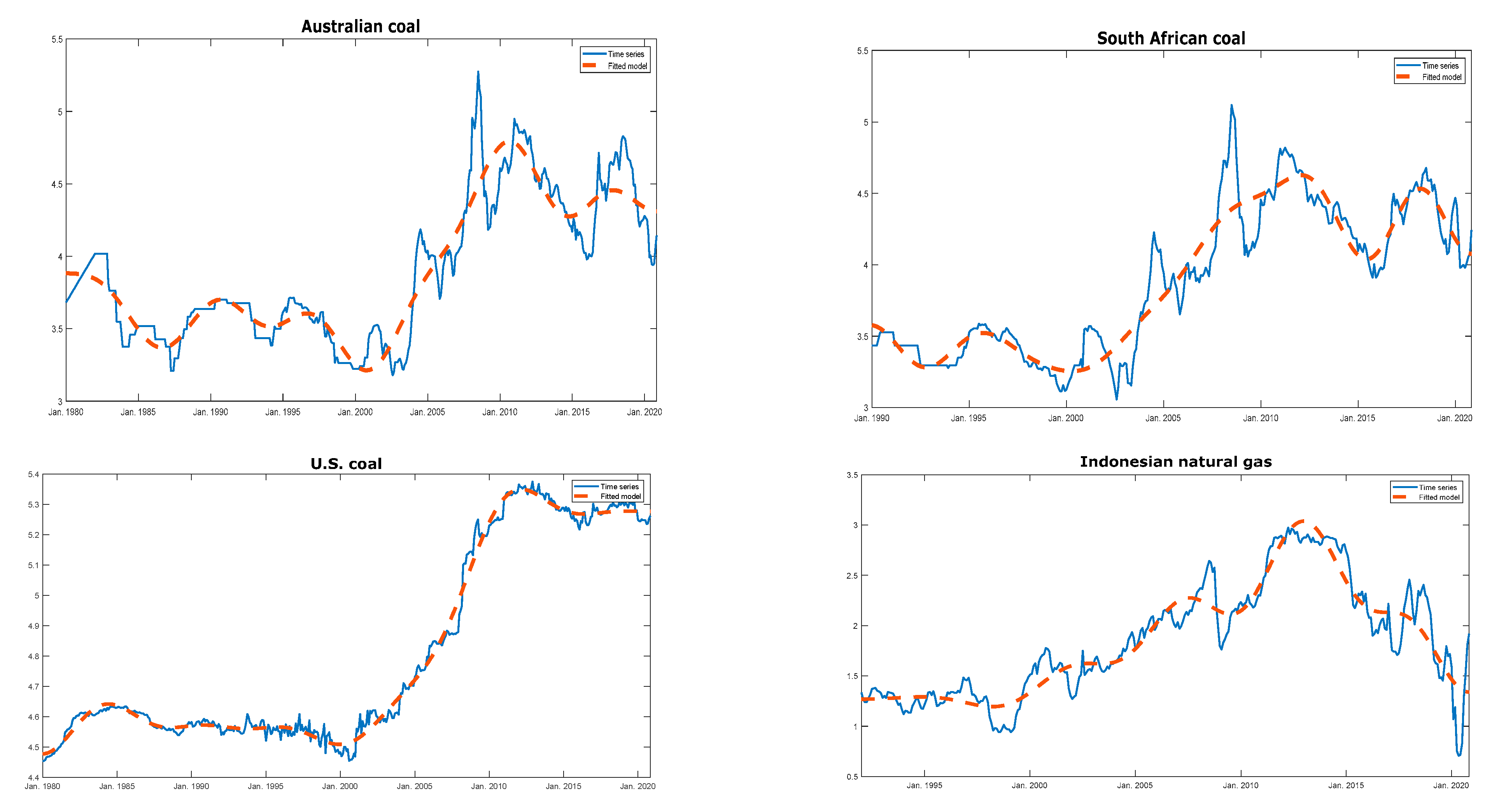
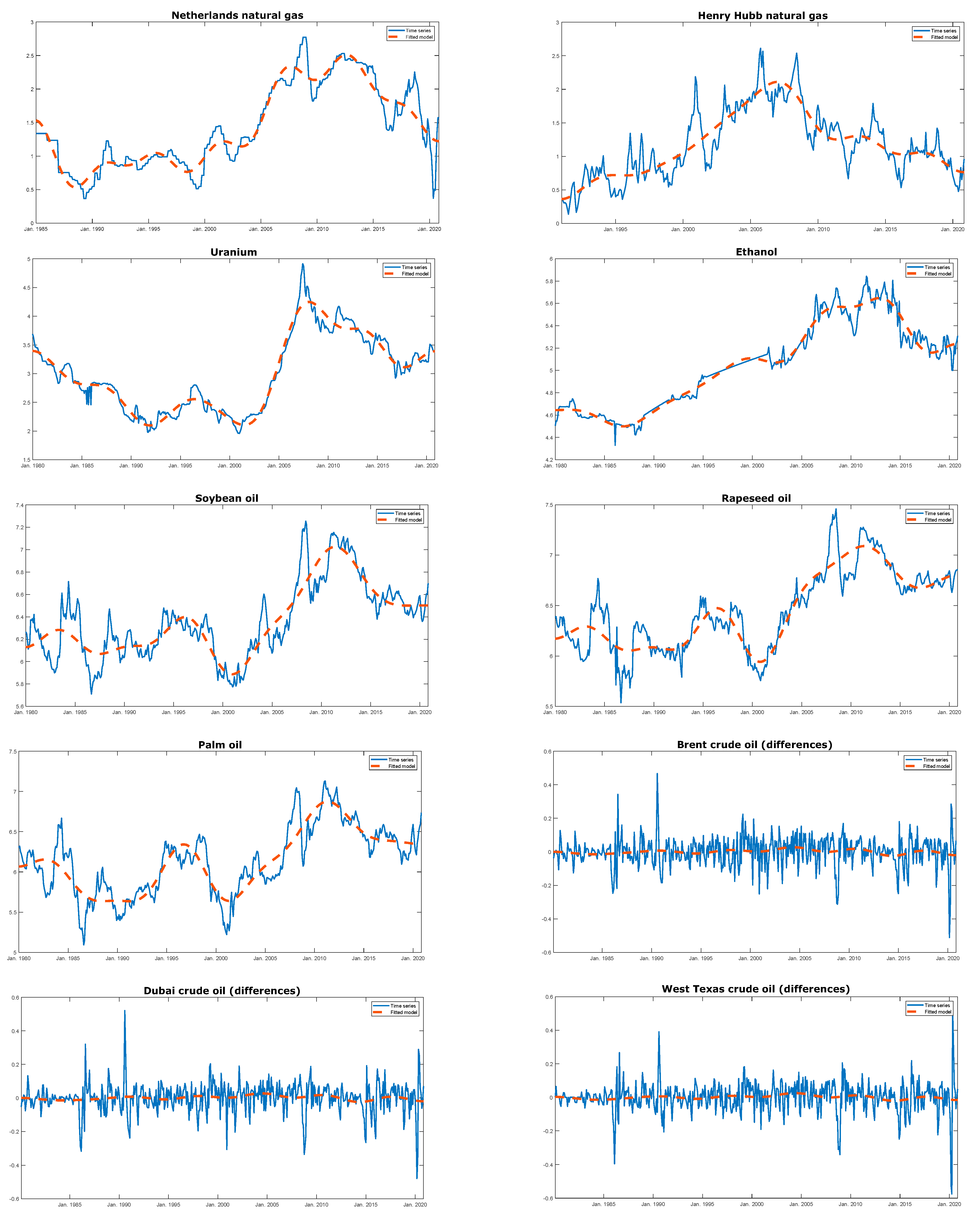
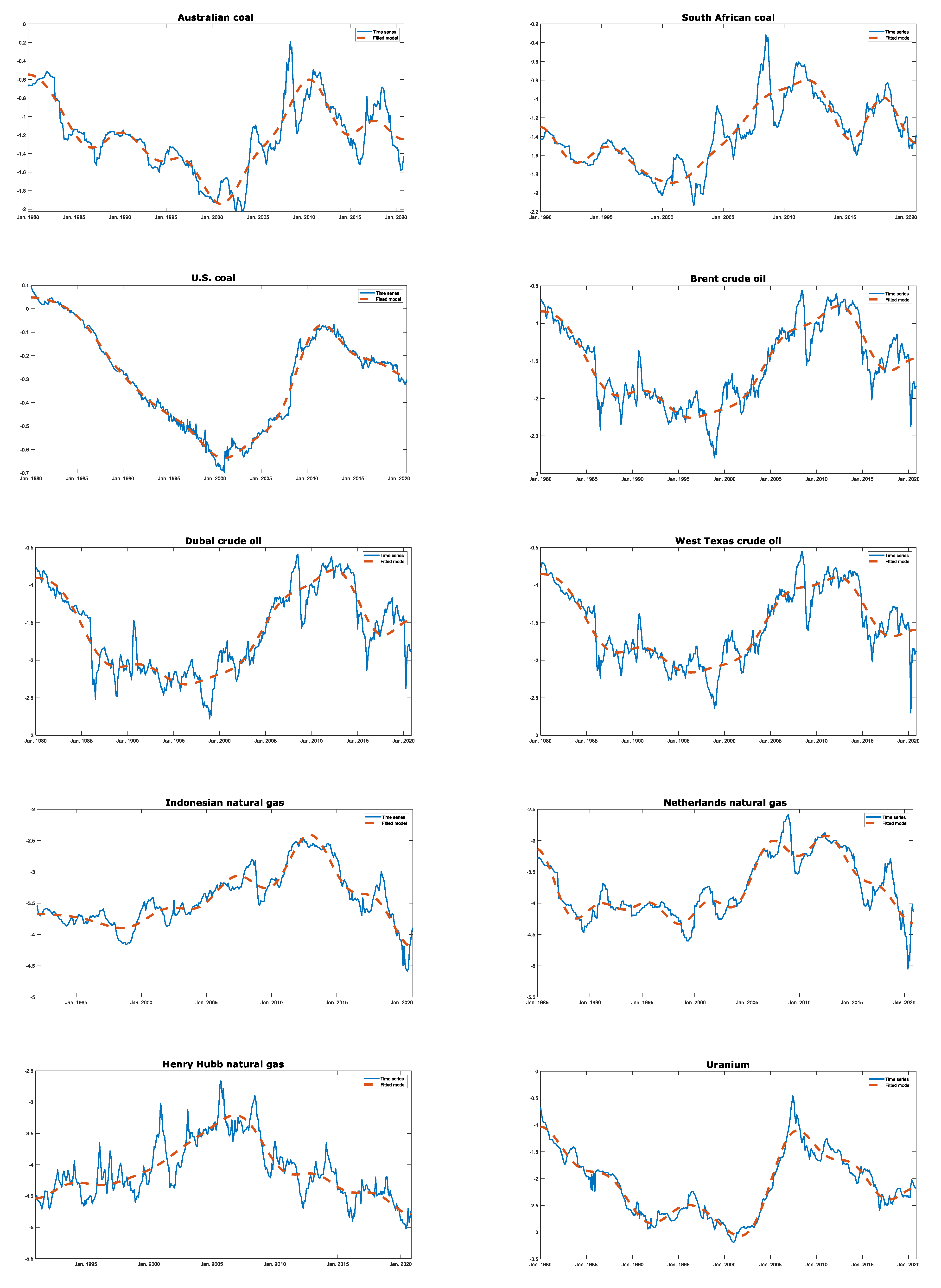
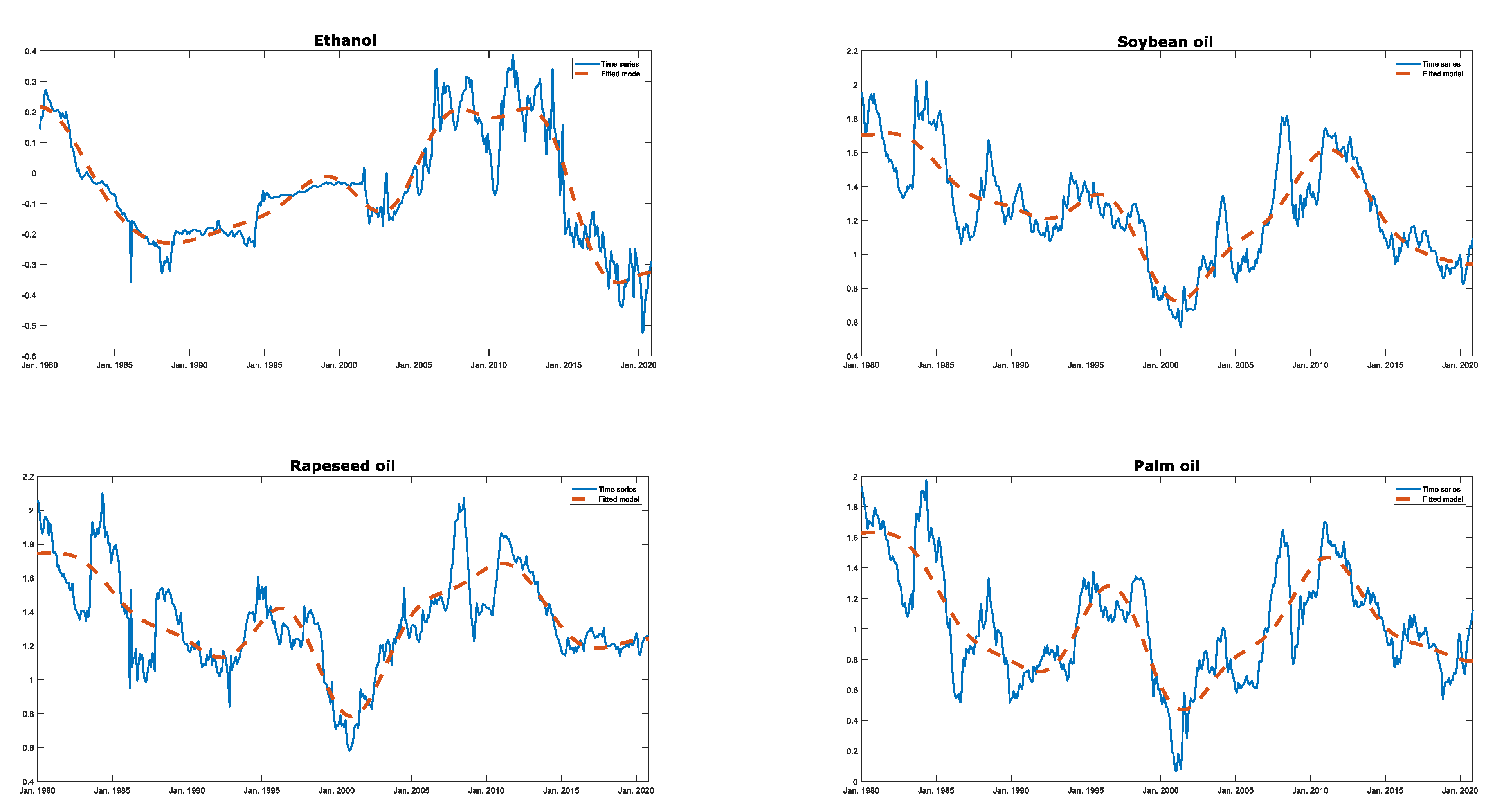
Figure 1 and Figure 2 below includes the plots of the series and their fitted nonparametric models (stationary cases) and the differenced series and their models (fitted on the differenced series) in those cases classified as nonstationary. For the sake of brevity, only the raw (Figure 1) and de-seasonalized, deflated (Figure 2) series are displayed.

5. Discussion

The conclusions of the various studies carried out by previous authors often differ (depending on the specific period analyzed, the frequency of data observed, and the methodology employed). In some of them, the possibility of non-linearities is explicitly considered and in others it is not, which can affect conclusions. In this regard, Chen and Lin [41] confirmed that the prices of coal, oil, and gas exhibit certain nonlinear features. Our non-parametric methodology automatically incorporates the possibility of non-linearities, so it would be naturally adapted to the analysis of these kinds of series.

As for coal, Lee et al. [42] and Presno et al. [4], employing PPI-deflated annual data, concluded that prices are stationary. The same conclusion is reached by Zaklan et al. [43], for annual data deflated by the U.S. CPI. However, Chen and Lin [41], employing a Markov switching unit root test, find non-stationarity in the monthly series of bituminous coal prices.

In the case of oil, Chen and Lin [41] concluded non-stationarity for the US West Texas Intermediate and UK Brent price series. This agrees with results by Maslyuk and Smyth [6], Tabak and Cajueiro [44], Alvarez-Ramirez et al. [45] (who also include the Dubai price in the analysis), and Lean et al. [46] (for the daily prices of WTI crude oil). Zaklan et al. [43] (for CPI-deflated annual data) concluded that the nature of oil prices shifted from stationary to integrated along the decade between late 1960s and late 1970s (regarding this possibility, it is interesting to note that our study period would be fully included in their non-stationary phase).

For natural gas, Chen and Lin [41] reported partial non-stationarity, with prices changing between local stationarity and local non-stationarity regimes. Zaklan et al. [43], employing CPI-deflated annual data, concluded stationarity.

Palm oil has been extensively analyzed in the literature on commodity prices. For instance, Ghoshray et al. [47], for annual data deflated by the MUV index, found stationarity. Harvey et al. [48] also concluded stationarity (around a quadratic trend) for that series. Our conclusions also agree with Lean and Smyth [21], who studied monthly spot and futures prices, finding little evidence to support the efficient market hypothesis. However, our findings would diverge from results by Lee et al. [24], who (for daily data) reported more efficiency in palm oil than in the West Texas Intermediate crude oil market, possibly explained by the smaller proportion of speculative transactions in the former as a consequence of relatively strict trading policies.

Results by Snaith et al. [23], who studied efficiency in the crude palm oil market (both in the open outcry and in electronic trading) by employing a threshold autoregressive relative efficiency measure, suggested an efficiency skew in that specific market. More precisely, they concluded long-run efficiency (in both trading platforms) for a vast majority of the maturities they tested, although some evidence of short-run inefficiency was also detected (with lower levels of short-run inefficiency in shorter maturities under open outcry and for longer maturities in electronic trading).

Our results for soybean oil differ from Chen et al. [25], although this might be a consequence of them employing ADF testing with no changes allowed for, as the power of that test is known to be potentially affected by the presence of breaks in the series. The same difference is observed in the case of uranium, where the models employed by Kahouli [28] and Chen et al. [25] did not allow for the possibility of breaks in the mean of the series. Finally, like Chang et al. [27], our results indicate that the prices of biofuels are stationarity.

6. Conclusions

In this paper, we analyzed non-stationarity in a group of fourteen, both renewable and non-renewable, energy commodity prices, for the 1980–2020 period. For many of these series, the presence of non-linear characteristics and breaks is well documented in the literature, with those factors adversely affecting the size and power of both stationarity and unit root tests. Our approach relies on a nonparametric, bootstrap-based stationarity testing framework that avoids the need of prior model specification for the deterministic components of the series analyzed.

Our analysis finds no statistically significant evidence to reject the trend-stationary nature of the price series analyzed, regardless of their renewable/non-renewable nature and the various data transformations considered. The only exception seems to be crude oil, for which unit roots are detected when the nominal and deflated prices are analyzed, although stationarity fails to be rejected when seasonal effects are taken into consideration. This highlights the importance of proper modeling of seasonal effects when analyzing commodity price series.

The above findings have several implications. First, our results would confirm–with the possible exception of oil prices—the assertions of economic theory on the dynamic behavior of commodity prices, in relation to the fact that market equilibria would suggest some form of stationary behavior in the time patterns of commodity prices. Based on our analysis, we cannot reject the hypothesis that, excepting oil, the prices of energy may follow a deterministic, Hotelling-type rule in the long run. The weak version of the efficient market hypothesis seemingly does not hold for those markets, with the mentioned exception of oil. This implies that the prices in those markets would tend to revert to their (generally time-varying) deterministic means, thus being predictable and manageable, with traders and investors in those commodities (and in the companies involved in their production) potentially being able to exploit technical analysis to make supra-normal profits.

Finally, although in this paper we have applied a mainstream de-seasonalizing treatment, a deeper theoretical analysis of seasonal filtering methods seems to be required in the case of nonparametric stationarity/unit-root testing.