Multiple (TEES)-Criteria-Based Sustainable Planning Approach for Mesh-Configured Distribution Mechanisms across Multiple Load Growth Horizons

Abstract

Modern distribution mechanisms within the smart grid paradigm are considered both reliable in nature and interconnected in topology. In this paper, a multiple-criteria-based sustainable planning (MCSP) approach is presented that serves as a future planning tool for interconnected distribution mechanisms and aims to find a feasible solution among conflicting criteria of various genres. The proposed methodology is based on three stages. In the stage 1, a weighted voltage stability index (VSI_W) and loss minimization condition (LMC) based approach aims at optimal asset optimization (sitting and sizing). In this stage, an evaluation of alternatives (solutions) is carried out across four dimensions (technical, economic, environmental, and social) of performance metrics. The assets considered in the evaluations include distributed generation (DG), renewable DGs, i.e., photovoltaic (PV), wind, and distributed static compensator (D-STATCOM) units. In the stage 2, various multicriteria decision-making (MCDM) methodologies are applied to ascertain the best trade-off among the available solutions in terms of techno-cost (economic) (TCPE), environment-o-social (ESPE), and techno-economic-environmental-socio (TEES) performance evaluations (OPE). In the stage 3, the alternatives are evaluated across multiple load growth horizons of 5 years each. The proposed MCSP approach is evaluated across a mesh-configured 33-bus active distribution network (ADN) and an actual NUST (which is a university in Islamabad, Pakistan) microgrid (MG), with various variants of load growth. The numerical findings of the proposed MCSP approach are compared with reported works the literature supports its validity and can serve as an important planning tool for interconnected distribution mechanisms for researchers and planning engineers.

1. Introduction

Worldwide electrical power demands have increased dramatically to meet the core requirements of modern societies. Among the three constituents of electrical power grids, namely generation, transmission, and distribution networks (DNs), the latter is pushed to operational limits, leading to technical and concerning issues of various kinds [1]. Competitive energy markets and deregulation regimes make it difficult to retain power grid performance, i.e., losses, voltage levels, and reliability indices, within an acceptable range. Conventionally, the DN paradigm has been deterministically designed to retain unidirectional power flow under radial topology, especially considering simple protection schemes and easy control [2]. In addition, traditional planning tools typically applied to radial DN planning (DNP) might not remain feasible to address the concerning issues of interconnected DNs and modernized infrastructure-based distribution mechanisms.

Limitations in existing DN infrastructure have forced power system stakeholders to incorporate new practices and concepts under the smart grid (SG) paradigm to evolve into smart DNs (SDNs). SDNs under SGs are considered reliable, secure, economic, environmentally friendly, and socially acceptable alternatives to the existing DN paradigm [3]. However, advanced distribution mechanisms require the support of various new optimization tools that aim at achieving multiple objectives of various genres and encapsulate future planning scenarios. It is mentioned in various works that an actual DNP problem aims to achieve a trade-off solution under several conflicting criteria subjected to various nonlinear system constraints [4].

The DN configuration constraint in most DNP problems considered with asset management (sitting and sizing) considers a radial configuration rather than one that is interconnected. The types of switches employed in DNs are either normally closed (NC) sectionalizing switches (SS) or normally open (NO) tie-switches (TS). The reconfiguration of the on/off status of these switches can transform the radial topology of a DN into an interconnected (loop or mesh) type in order to distribute loadings among various feeders and ensure reliability and improvement in voltage profile [5]. Likewise, the incorporation of assets, predominantly distributed generation (DG) unit integration, was not considered at the planning stage, nor assisted in the operational phase of the radial structured distribution network (RDN) in the traditional grid paradigm. However, DG asset integration has transformed the passive nature of DNs to one that is active, called active DN (ADN). The ADN manages systems in an efficient manner compared to its “fit and forget” counterpart [6].

Optimal asset placement (OAP) in interconnected configured DNs, i.e., loop DN (LDN) or mesh DN (MDN) under ADN management, enables reliability and better services [7]. Moreover, future distribution mechanisms under the SG paradigm are envisioned as interconnected, reliable, and offering a variety of options, limited in existing DN infrastructure. These various features of SGs have given way to interconnected configured distribution mechanisms such as loop/mesh-configured DNs and microgrids (MGs) [8]. Such ADN and MG setups are the most suitable option for densely populated urban centers, employing modernization of existing infrastructure. Besides LDNs and MDNs, MG is a concept that envisions several aspects of the grid in which a portion of the overall grid has defined electrical boundaries along with a means of energy production with DGs and management of concerning loads. Interconnected MGs can offer an efficient distribution alternative for multigeneration and load management to ensure reliable services [9].

DN modernization under SG encapsulates several aspects that require decision-making (DM) tools and techniques in order to provide a compact solution under various confliction criteria, as modern planning techniques cover several criteria that belong to various genres. Moreover, besides technical and economic criteria, the geographical spread of the new mechanism requires evaluation across environmentally friendly and socially acceptable solutions. Hence, the number of possible solutions (or alternatives) must be evaluated across multidimensional criteria (objectives) to arrive at a win–win situation for all stakeholders [10].

Traditional asset optimization approaches in DNs aim specifically to find an alternative with minimum optimal cost. However, such techniques lack a solution that fits across all requisite rubrics. Moreover, the radiality constraint is one of the most important features of respective traditional RDNs [11]. In the literature, DNP-centric asset optimization within system constraints mostly aims at the sitting and sizing of individual assets, i.e., DGs (conventional and renewable), reactive power (Q) compensation devices such as capacitors and distributed static compensators (D-STATCOM), and grid reinforcements, along with topology change within DNs [12,13]. Objectives accredited on the technical side primarily include minimizing system active/reactive power losses, voltage profile improvement, optimal DG (primarily renewable energies generation (REG)) penetration, power quality, short-circuit levels, acceptable bidirectional power flows, and overall system stability. Economic objectives mainly include an increase in profitability and savings, along with a reduction in the cost of system losses and operational, running, and maintenance costs. The aimed solutions are anticipated to achieve objectives that are feasible environmentally and acceptable socially.

The literature review further indicates that various techniques are utilized to achieve the above-mentioned objective of various genres. Prominent techniques include classical (exhaustive research, numerical, analytical, deterministic, etc.), nature (people or society)-inspired heuristic (and meta-heuristic), artificial-intelligence-inspired neural networks, improved hybrid variants, and commercial solvers. However, such techniques (or algorithms) are utilized to achieve a solution that may lead to local optima in various scenarios and cases [2,3,4,10,11,12,13]. The case may worsen if the number of objectives (or criteria) increases, and computation costs may increase further. This particular limitation is generally linked to hybrid algorithms aimed at global optima. In addition, multicriteria (also called multi-attribute) decision-making (MCDM) techniques are used to sort a compromise solution between various relevant criteria/objectives of contradictory nature [4,14]. Such methods can be optimized a priori by assigning weights (subjectively or objectively) to each criterion (a priori methods) or applied subsequently (posteriori methods) to a varied number of solutions resulting from internal optimization [15].

From the modern DNP viewpoint, several researchers have conducted studies in various dimensions, i.e., DN reconfiguration, asset optimization across planning horizons, efficient management with ADN techniques, multi-criteria (multi-objective)-based optimizations, interconnected LDN/MDN, and MG planning and scheduling as prominent examples [9,10,16,17]. Interconnected ADNs, i.e., LDNs/MDNs and interconnected MGs, are not as prevalent as their radially configured counterparts [5,6,7,8,18]. Therefore, to meet the future requirements of urban centers, they should be considered from the perspective of planning, in particular grid modernization. Moreover, interactions between power production, distribution mechanism dynamics, concerning policies, environmental concerns, and societal benefits have dynamically nonlinear characteristics. Hence, the sustainable modernization and development of the anticipated complex distribution mechanism require a long-term planning solution evaluated across multiple criteria that are contradictory in nature.

Researchers around the world have made several attempts to address the aforementioned limitations in asset planning across various distribution mechanisms. The methodologies sort out a trade-off solution between conflicting objectives that may spread across various dimensions. These trade-off solutions may be of a genre that refers to technical, economic, environmental, and social solutions, either addressed individually or in combination with a couple of multidimensional objectives [19]. Works based on MCDM techniques have been performed aimed at evaluations in terms of criteria such as techno-economic [20,21,22,23,24], economic only [25,26], and economic-environmental [27], catering to REGs in mostly isolated DNs. On the axis of grid-connected ADNs, several works such as [28,29,30,31,32,33] based on MCDMs have aimed at addressing mostly technical and economic objectives, yet considering radiality constraints and across normal load conditions without considering large-scale planning horizons. A simultaneous techno-economic-environment-based approach was conducted across normal loading scenarios only in [34] at various power factors (PF) associated with REGs in radially configured ADNs.

LDN/MDN-configured ADNs have been reviewed with indices-based asset optimization methods, i.e., analytical/numerical and hybrid techniques [5,6,7,8,9,16,17,18,35,36,37,38,39,40]. These methodologies mostly aim at techno-economic objectives such as loss minimization (LM), voltage profile stabilization (VPS), DG penetration (DGP), reliability, and concerning cost indices. The prime assets considered are DGs, REGs, and Q-compensation devices such as D-STATCOM. However, environmental and social concerns were not addressed. LDN/MDN infrastructure-based optimization has considered various strengths of the number of TS and its influence on different load levels, as well as an evaluation of load growth horizons. DN configuration reinforcement with looping/meshing and optimal use of DSTATCOM in interconnected DNs has been considered in the reviewed works. Optimal planning of D-STATCOM is accredited with increasing REG-based DG penetration, voltage stabilization (VS), loss minimization (LM), and reduction of associated cost targets. Technical index-based multicriteria methodologies have been applied for asset planning with DGs in LDN aimed at technical objectives [35,36] under normal load and techno-economic load across the load growth [37,38]. The MCDM methods used in the above-mentioned works [35,36,37,38] include the weighted sum method (WSM), the weighted product method (WPM), and the technique for order preference by similarity to ideal solution (TOPSIS).

The study in [39] reviewed voltage stability indices (VSI) evaluated across radially configured DGs and encompasses the technical perspective only. In recent work reported in [40,41] for MDNs, two different variants of an integrated planning approach integrating an improved voltage stability assessment indices (VSAI), also interchangeably used as VSI, (designated as VSAI_A and VSAI_B or simply VSI_A and VSI_B), as well as the loss minimization condition (LMC), were used for optimal optimization of assets in MDNs such as DGs only and REG-D-STATCOM sets for techno-economic targets under normal load. However, VSIs in [40,41] have conflicting critical criteria of stability and exhibit utilization issues when considered simultaneously. Another improved variant of [41] based on VSI_B and LMC followed by MCDMs in terms of the integrated decision-making planning (IDMP) approach in [42] was evaluated across techno-economic criteria considering a planning horizon of five years. The MCDM methods used in [42] include WSM, WPM, the Technique for Order of Preference by Similarity to Ideal Solution (TOPSIS), and the Preference Ranking Organization Method for Enrichment of Evaluations (PROMETHEE), which are evaluated in terms of unanimous decision-making scores.

The world is moving toward the research dimension of DN modernization, which refers to distribution mechanisms of interconnected nature to ensure reliability while abiding by nonlinear system constraints. Asset management in interconnected ADNs is a suitable alternative to the “fit and forget approach” in respective radial counterparts, aiming at the achievement of multiple conflicting criteria spread across multiple dimensions across certain planning horizons. Likewise, LDN, MDN, and interconnected MGs have been evaluated as suitable ADNs as suitable candidates of SDNs, evaluated across mostly techno-economic criteria. Looped MGs have been evaluated across technical perspectives in the reviewed works.

However, in the above-mentioned works, mostly techno-economic criteria have been considered rather than environmental and social counterparts across interconnected MDNs and MGs, which are suitable candidates of SDNs. No such work has been evaluated across multiple planning horizons. The reviewed works partially address the above issues from various perspectives and partly bridge the limitations. The very aim of this paper is to bridge the limitations as motivation in the reviewed works and offer a composite integrated asset planning framework that serves the very novelty of the proposed work. Hence, the very framework offers a complete multiple-criteria evaluation encompassing notable dimensions across multiple planning horizons to ensure sustainability. Moreover, modern SDN-based planning requires upgradation that must provide criteria to be evaluated across multiple dimensions rather than only one dimension.

In this paper, an improved integrated decision-making planning referred to as multi-criteria (TEES)-based sustainable planning (MCSP) approach is proposed that aims to evaluate multiple criteria in multiple dimensions across multiple planning horizons. The proposed approach encompasses initially proposing an improved weighted variant of VSI to mitigate conflicting critical stability index criteria, designated as VSI_W (for asset sitting) and followed by LMC (for asset sizing). Later, various MCDM methodologies (WSM, WPM, TOPSIS, and PROMETHEE) are applied across multiple load growth horizons to sort out trade-off solutions across various alternatives. The proposed MCSP approach is applied across a 33-bus MDN and mesh-configured microgrid (MCMG) based on an actual on-ground system. The assets optimized in the proposed MCSP approach extend across DGs at a lagging PF capable of contributing both active (P) and Q powers and a REGs-DSTATCOM set such as photovoltaics (PVs) contributing P and Q, respectively. The approach is capable of providing alternatives across criteria pertaining to seven dimensions, namely technical only, economic only, environmental only, social only, techno-economic, environment-o-social, and techno-economic-environmental-socio (TEES). Likewise, the proposed MCSP approach can serve as an important future planning tool for interconnected ADN mechanisms for researchers and planning engineers from the SDN perspective of the smart grid paradigm. The main contributions of the proposed works are as follows:

(i)

Multi-criteria (TEES)-based sustainable planning (MCSP) approach for optimal asset optimization.

(ii)

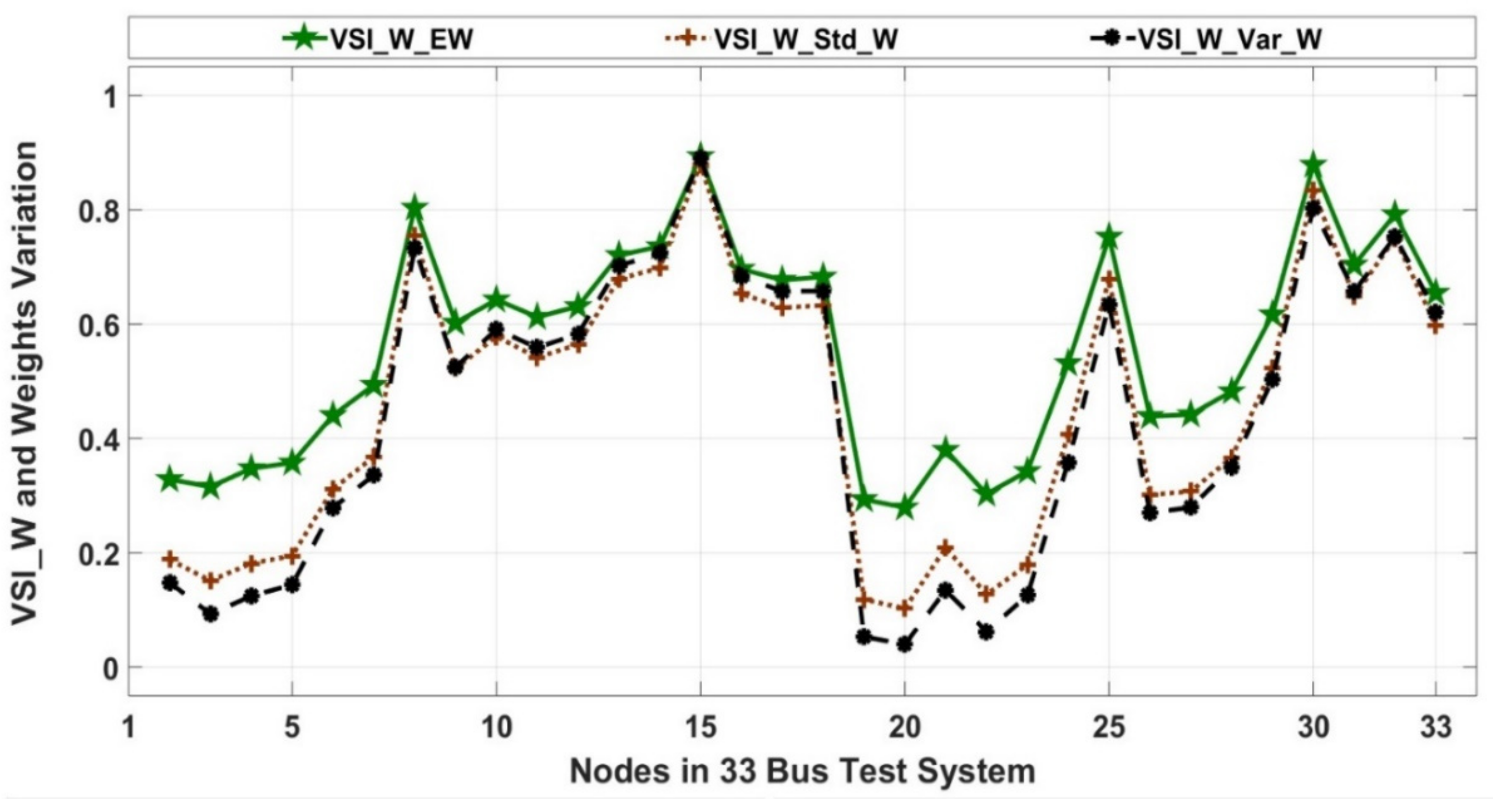
Evaluation of multiple assets (sitting and sizing) with VSI_A-LMC, VSI_B-LMC, and the proposed VSI_W-LMC.

(iii)

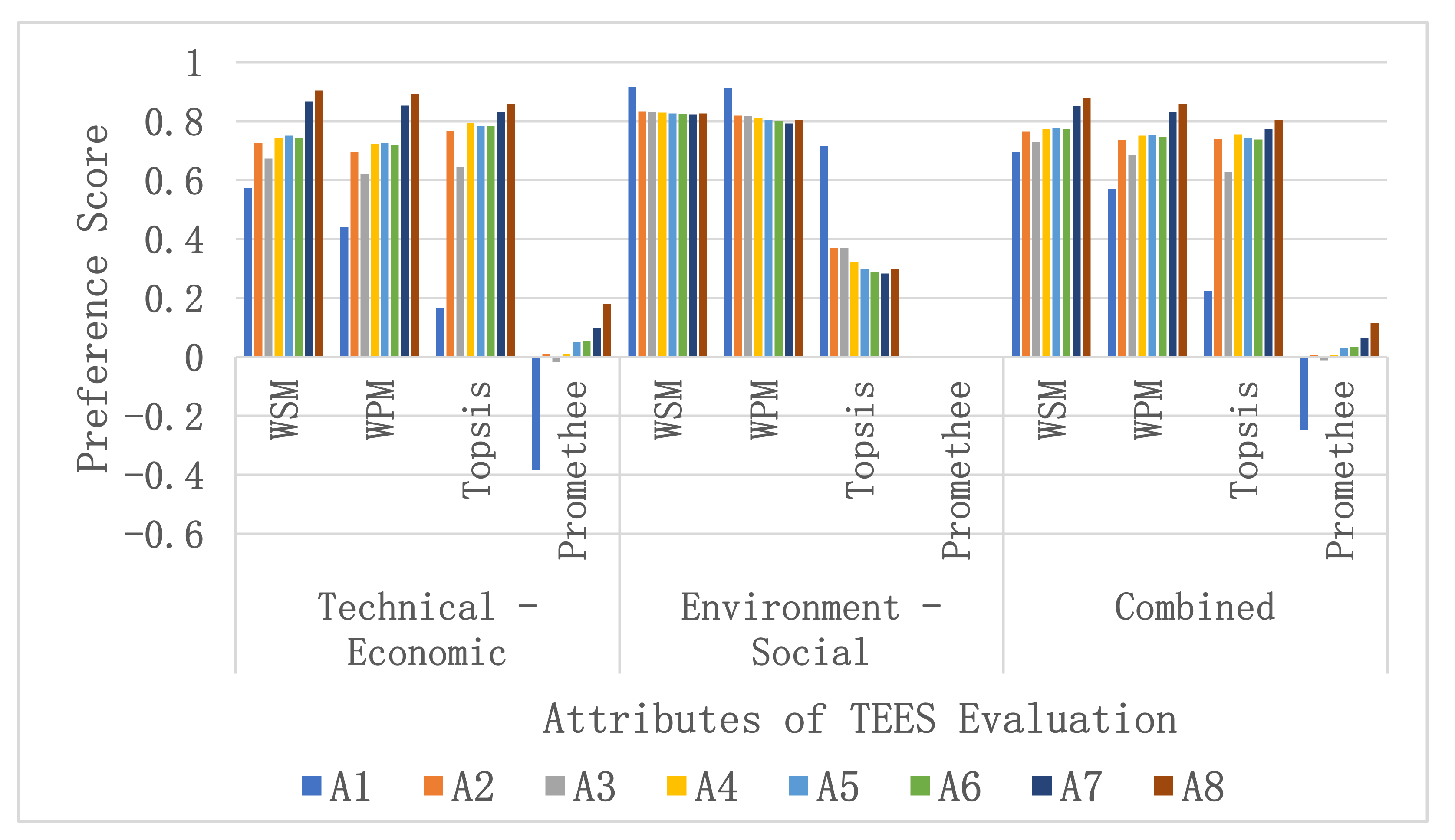
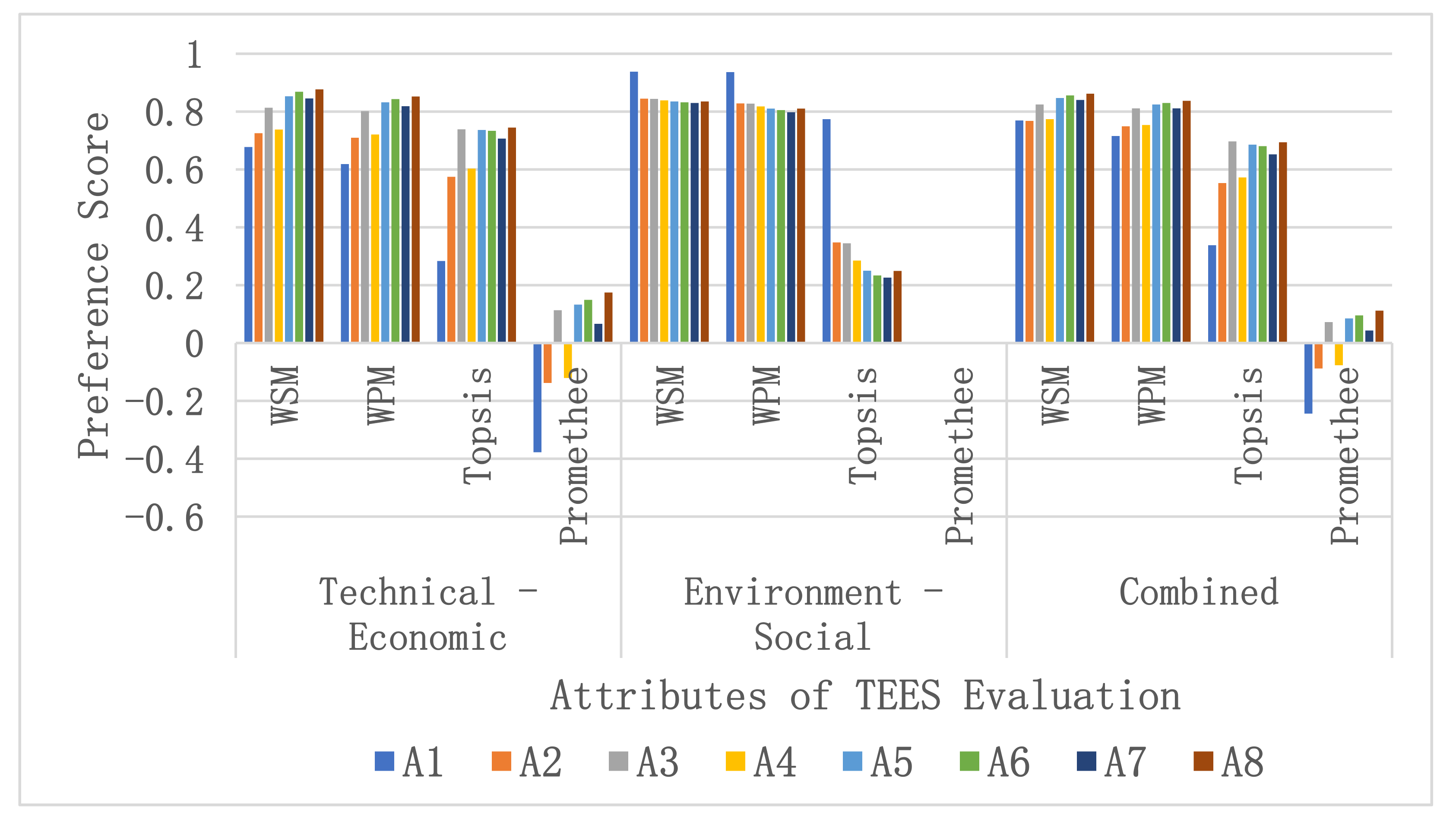
Evaluation of alternatives (solutions) across various dimensions of performance metrics.

(iv)

Evaluation with techno-economic-environmental-social performance metrics.

(v)

Comprehensive alternatives evaluation across multiple load growth horizons.

(vi)

Detailed evaluation of trade-off alternatives across multiple sets of solutions.

(vii)

Numerical evaluations were conducted across a 33-bus MDN and an actual MCMG.

(viii)

Consideration of the impact of expansion-based planning and new nodes across planning horizons.

(ix)

Validation of achieved results with those reported in the literature as a benchmark.

This paper is arranged as follows. Section 2 presents the proposed MCSP along with respective mathematical expressions and computational procedures. The simulation setup and performance evaluation indices are shown in Section 3. Section 4 gives a detailed account of the proposed approach’s effectiveness across multiple assets and respective performance evaluations across multidimensions and multiple load growth planning horizons. Benchmarking and validation analysis are shown in Section 5. Finally, the paper is concluded in Section 6.

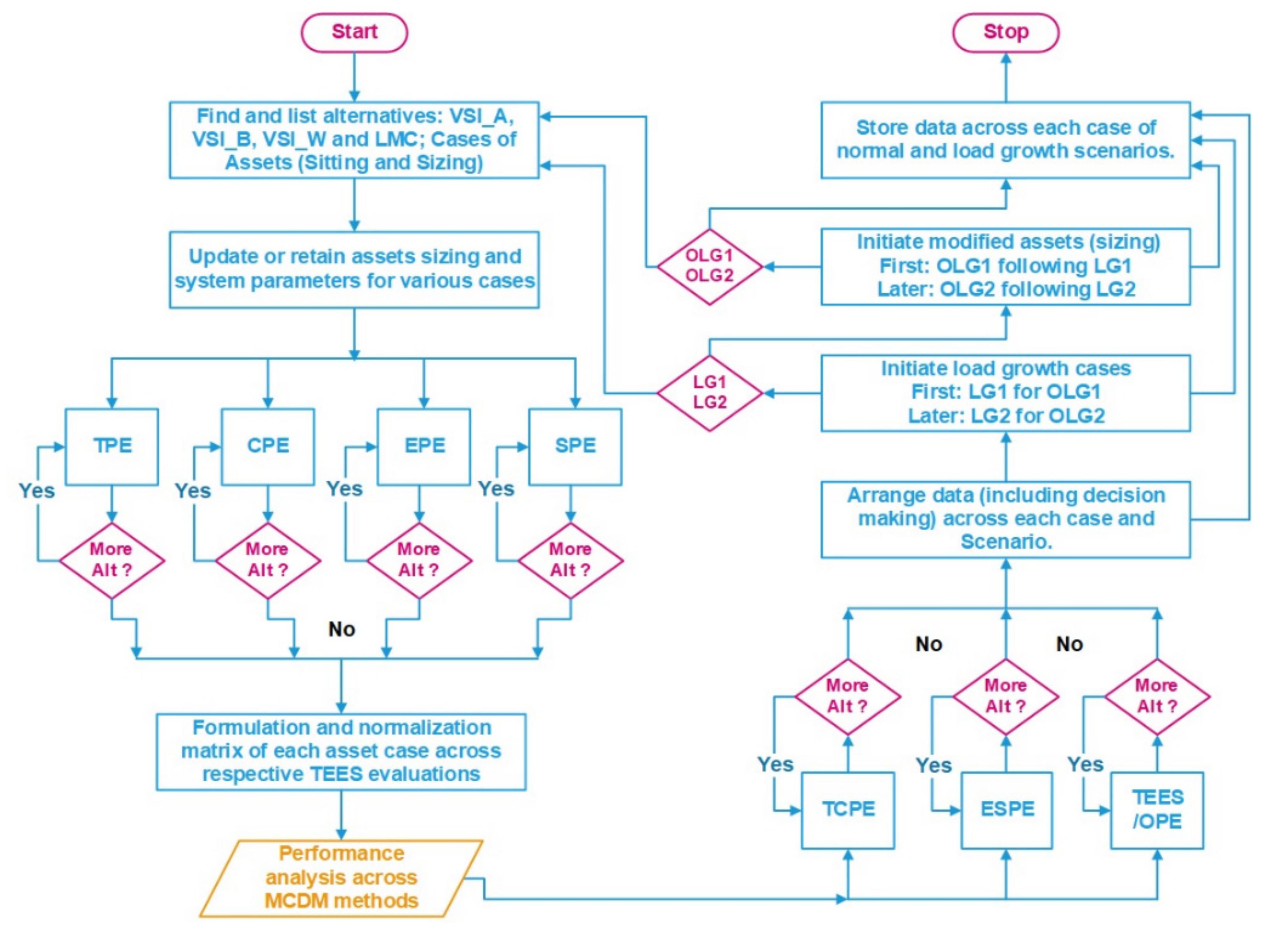
2. Proposed Multi-Criteria-Based Sustainable Planning (MCSP) Approach

The electrical equivalent of the MDN shown in Figure 1 consists of three branches representing each feeder of the test DN with two closed tie-lines (TLs) for linkage in the mesh configuration. The voltages from the sending end nodes/buses (n_1b, n_3b, and n_5b) are assumed to exhibit the same magnitude and phase angle (δ) and are represented as one source node/bus n_1b. The receiving end nodes/buses (n_2b, n_4b, and n_6b) are connected via two closed TLs. The loads S_2b, S_4b, and S_6b at n_2b, n_4b, and n_6b are considered the summed lumped load (S_2B = P_2B + jQ_2B) at bus/node m_2b with a voltage magnitude of V_2b, as shown in Figure 1 [40,41,42].

In this paper, the methodology is based on three stages. In the stage 1, the weighted VSAI based on three VSI indices (VSAI), formulated in previous publications by the author [40,41,42], and voltage deviation/profile improvement index in [32] are utilized for optimal sitting of the assets. Later in the stage 1, the loss minimization condition (LMC) is incorporated, which considers the optimal sizing of the assets as possible solutions. In the stage 2, various MCDM techniques are utilized to find the best solutions among those available. In the stage 3, multiple load growth scenarios across planning horizons are evaluated across multicriteria of various dimensions to ascertain the best overall solution with various types of assets in different test systems.

In the stage 1, VSAIs in [40,41] are designated as VSI_A and VSI_B. Both aim at optimal asset sitting. The threshold value of VSI_A, expression shown in Equation (1), lies between 0 (instability) and 1 (stable). The expression of VSI_B, as illustrated in Equation (2), has a threshold value, unlike VSI_A, between 1 (instability) and 0 (stable). The VSI_D in Equation (3) must exhibit a positive value, and the numerical value based on the highest deviation shows the critical loading condition of a bus/node in a distribution network close to the voltage collapse.

$$VSI\_A={\displaystyle \sum }_{i=1}^{n_l}{\left(\frac{V_{sb}}{n}\right)}^4-\frac{4}{n}{\displaystyle \sum }_{i=1}^{n_l}{\left(\frac{V_{sb}}{n}\right)}^2\left[\left(\frac{A_A}{C_A}\right)+\left(\frac{B_A}{D_A}\right)\right]-\frac{4}{n^2}{\left[\left(\frac{A_A}{C_A}\right)-\left(\frac{B_A}{D_A}\right)\right]}^2\ge 0$$

(1)

where

$$A_A=P_{2B} \left[{\displaystyle \prod }_{i=1}^n{R}_{nr}\right]\left[1-\left(\frac{X_{1x}{X}_{2x}}{R_{1r}{R}_{2r}}+\frac{X_{1x}{X}_{3x}}{R_{1r}{R}_{3r}}+\frac{X_{2x}{X}_{3x}}{R_{2r}{R}_{3r}}\right)\right]+ Q_{2B} \left[{\displaystyle \prod }_{i=1}^{n}nx\right]\left[\left(\frac{R_{1r}{R}_{2r}}{X_{1x}{X}_{2x}}+\frac{R_{1r}{R}_{3r}}{X_{1x}{X}_{3x}}+\frac{R_{2r}{R}_{3r}}{X_{2x}{X}_{3x}}\right)-1\right]$$

$$B_A=P_{2B}\left[{\displaystyle \prod }_{i=1}^n{X}_{nx}\right] \left[\left(\frac{R_{1r}{R}_{2r}}{X_{1x}{X}_{2x}}+\frac{R_{1r}{R}_{3r}}{X_{1x}{X}_{3x}}+\frac{R_{2r}{R}_{3r}}{X_{2x}{X}_{3x}}\right)-1\right]-Q_{2B} \left[{\displaystyle \prod }_{i=1}^n{R}_{nr}\right]\left[1-\left(\frac{X_{1x}{X}_{2x}}{R_{1r}{R}_{2r}}+\frac{X_{1x}{X}_{3x}}{R_{1r}{R}_{3r}}+\frac{X_{2x}{X}_{3x}}{R_{2r}{R}_{3r}}\right)\right]$$

$$C_A \left[abs\left\{\sum _{k\ne l}^n{R}_k{R}_l-\sum _{k\ne l}^n{X}_k{X}_l\right\}+0.001\right];$$

$$D_A=abs\left(R_1{X}_2+R_2{X}_1+R_1{X}_3+R_3{X}_1+R_2{X}_3+R_3{X}_2\right)=abs\left[\sum _{k\ne l}^n{R}_k{X}_l\right]$$

$$VSI\_B=4n^2\frac{\left[E_B{{\displaystyle \sum }}_{i=1}^{n_l}{\left(\frac{V_{sb}}{n}\right)}^2+{\left(\frac{F_B}{n}\right)}^2\right]}{{{\displaystyle \sum }}_{i=1}^{n_l}{\left(\frac{V_{sb}}{n}\right)}^4} \le 1$$

(2)

where

$$E_B=\left[abs\left\{\left(P_{2b}{R}_{1r }+P_{4b}{R}_{2r }+P_{6b}{R}_{3r }\right)+\left(Q_{2b}{X}_{1x}+Q_{4b}{X}_{2x}+Q_{6b}{X}_{3x}\right)\right\}+0.001 \right]$$

$$F_B=\left[abs\left\{\left(P_{2b}{X}_{1x}+P_{4b}{X}_{2x}+P_{6b}{X}_{3x}\right)-\left(Q_{2b}{R}_{1r }+Q_{4b}{R}_{2r }+Q_{6b}{R}_{3r }\right)\right\}+0.001 \right]$$

$$VSI\_D={\displaystyle \sum }_{i=1}^{n_l}{\left(V_{sb}-V_{rb}\right)}^2 \ge 0$$

(3)

where V_sb is the reference voltage value of the sending end node/bus, i.e., substation voltage.

V_rb is the voltage value of the receiving end node/bus throughout the test DN.

The weighted VSI index is designated as VSI_W and is based on weighted normalized values of VSI_An, VSI_Bn, and VSI_Dn, shown in Equation (4), as follows:

$$VSI\_W=\left[\left({\omega }_A\times VSI\_An\right)+\left({\omega }_B\times VSI\_Bn\right)+\left({\omega }_D\times VSI\_Dn\right)\right]$$

(4)

where ${\omega }_A,{\omega }_B,{\omega }_D$ are the weights of each individual normalized values of VSI, and their sum is equal to one.

Weights were allocated in equal proportions and on the basis of the standard deviation and variance trends of the respective VSIs.

Later in the stage 1, the method of LMC remains the same as in both VSI_A [40] and VSI_B [41] for their proposed counterpart VSI_D in the MCSP approach. Modified expressions for LMC for active (P_Loss) and reactive power losses (Q_Loss) when tie-line and loop currents are zero are shown in Equation (5) as LMC_P and LMC_Q in Equation (6), respectively [40,41,42].

$$LMC\_P=\left[{\left(I_{2B}\right)}^2{R}_{2r}+{\left(I_{1B}\right)}^2{R}_{1r}+{\left(I_{3B}\right)}^2{R}_{3r} \right]\ge 0$$

(5)

$$LMC\_Q=\left[{\left(I_{2B}\right)}^2{X}_{2x}+{\left(I_{1B}\right)}^2{X}_{1x}+{\left(I_{3B}\right)}^2{X}_{3x}\right]\ge 0$$

(6)

where $I_{1B}, I_{2B}, I_{3B}$ are the respective line current across each feeder in the MDN, $R_{1r}, R_{2r}, R_{3r}$ are the respective line resistance across each feeder in the MDN, and $X_{1x}, X_{2x}, X_{3x}$ are the respective line reactance across each feeder in the MDN.

The performance evaluation across various alternatives was assessed across the dimensions of technical, cost-economic, environmental, and social perspectives. The respective performance indicators were designated with a technical performance evaluation (TPE), cost-economic performance evaluation (CPE), environmental performance evaluation (EPE), and social performance evaluation (SPE).

In the stage 2, after multi-criteria decision-making (MCDM), approaches such as WSM, WPM, WPM, and PROMETHEE as the priori methods, with subjectively assigned weights, are individually applied to each criterion of multiple dimensions (after normalization) for respective alternatives after the formulation and normalization of the decision matrix across each asset. For respective details, refer to the authors’ previous publication [42]. The generic decision matrix in MCDM is shown in

Table 1. Generic decision matrix in MCDM methodologies.

Solutions (S)/Alternatives (A)	Weighted Attributes (w) across Criterion (C)
	w1*C1	w2*C2	w3*C3	…	wY*CZ
S1	A11	A12	A13	…	A1Z
S2	A21	A22	A23	….	A2Z
S3	A31	A32	A33	…	A3Z
…	…	…	…	…	…
SX	AY1	AY2	AY3	…	AYZ

. Normalization helps enable a standard unified scale for measurement and analysis, as shown in Equation (7). The decision matrix Sxz is normalized using Equation (7) for the respective criterion Cxz to increase (positive) or decrease (negative).

$$S_{xz}^{-}=\frac{Mi{n}_{A^Y\in A} C_{xz} }{ C_{xz} } ; S_{xz}^{+}=\frac{ C_{xz} }{Ma{x}_{A^Y\in A} C_{xz} }$$

(7)

The weights in Table 1 in each MCDM method are considered unbiased (or equal) weights. All the alternatives and the trade-off final solution achieved are subjected to practical system constraints. The individual TPE-, CPE-, EPE-, and SPE-based evaluations are followed by techno-economic (cost) (TCPE), environmental-social (ESPE), and overall (TEES) performance evaluation (OPE), as per MCDM methods.

The unanimous decision-making score (UDS) shown in Equation (8) is followed across each MCDM technique [42]. This UDS determines the highest rank on the basis of the highest numerical value and is designated here as a unanimous decision-making rank (UDR), as shown in

Table 2. Rank and score provision for the unanimous decision-making score (UDS) [42].

Alternatives Rank (AR)	Alternatives Score (AS)
(Highest to Lowest)	Highest (H) to Lowest
A1R = 1	H
A2R = 2	H-1
A3R = 3	H-2

. If two UDR scores are equal, the one with the highest UDS will be given preference. To speed up the decision-making (DM) process, the UDS of only the three highest scores are considered for final scores and further evaluations.

$$UDS={\displaystyle \sum }_{M=1}^{n=k}\left(A_R\times \frac{A_S}{A_R} \right)={\displaystyle \sum }_{M=1}^{n=k}\left(A_S\right)$$

(8)

In the stage 3, multiple load growth scenarios across planning horizons are evaluated across multicriteria of various dimensions to ascertain the best overall solutions with various types of assets in different test systems. The planning horizon can be from 2 to 5 years, depending upon the type of evaluation mechanism under evaluation. The assets include renewable DGs (REGs), conventional DGs, and D-STATCOM. A flow chart of the proposed multi-criteria-based sustainable planning approach is shown in detail in Figure 2.

3. Test Setups, Computational Procedure, and Evaluation Indices

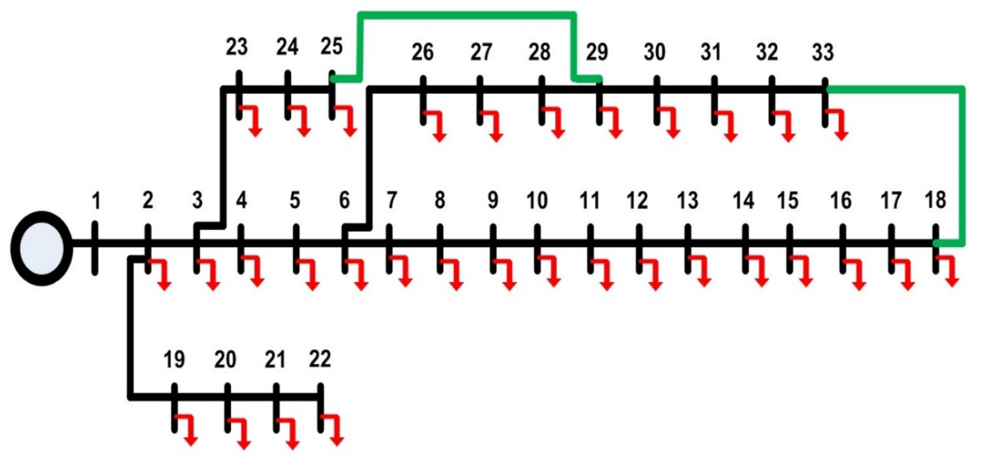
3.1. Mesh-Configured 33-Bus Active Distribution Network

The proposed MCSP approach was tested on two mesh-configured distribution mechanisms. The first is a mesh-configured 33-bus test distribution network (TDN), as shown in Figure 3. Evaluations for an ADN were carried out on a 33-bus MDN, which has an active (P_LD) and reactive load (Q_LD) of 3715 KW and 2300 KVAR and active (P_Loss) and reactive losses (Q_Loss) of 210.9 KW and 143.02 KVAR, under NL, respectively. For LG1, the P_LD and Q_LD are 5333.363 KW and 3301.95 KVAR, respectively. The P_Loss and Q_Loss (during LG1) account for 450.65 KW and 305.17 KVAR, respectively. For LG2, the P_LD and Q_LD are 7656.73 KW and 4740.38 KVAR, respectively. The P_Loss and Q_Loss during LG2 account for 1111.251 KW and 752.52 KVAR, respectively. All the setups were developed in the MATLAB/Simulink (R2018a) environment. The test MDN consists of four branches and five TSs. The 33-bus TDN was converted into a multiple-loop-configured MDN by closing TS4 and TS5 (highlighted in a green solid line) and resulted in two loops (or a mesh configuration).

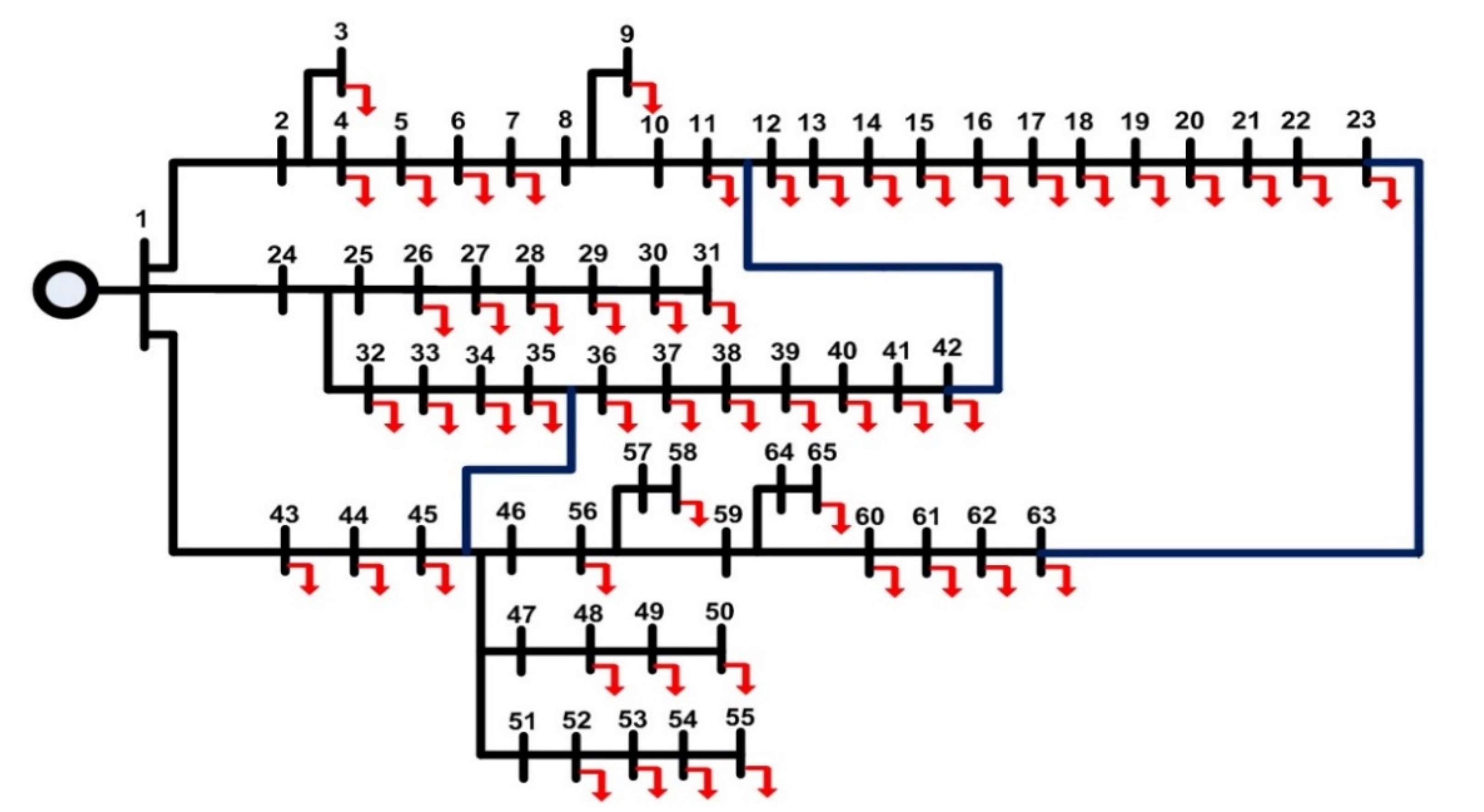
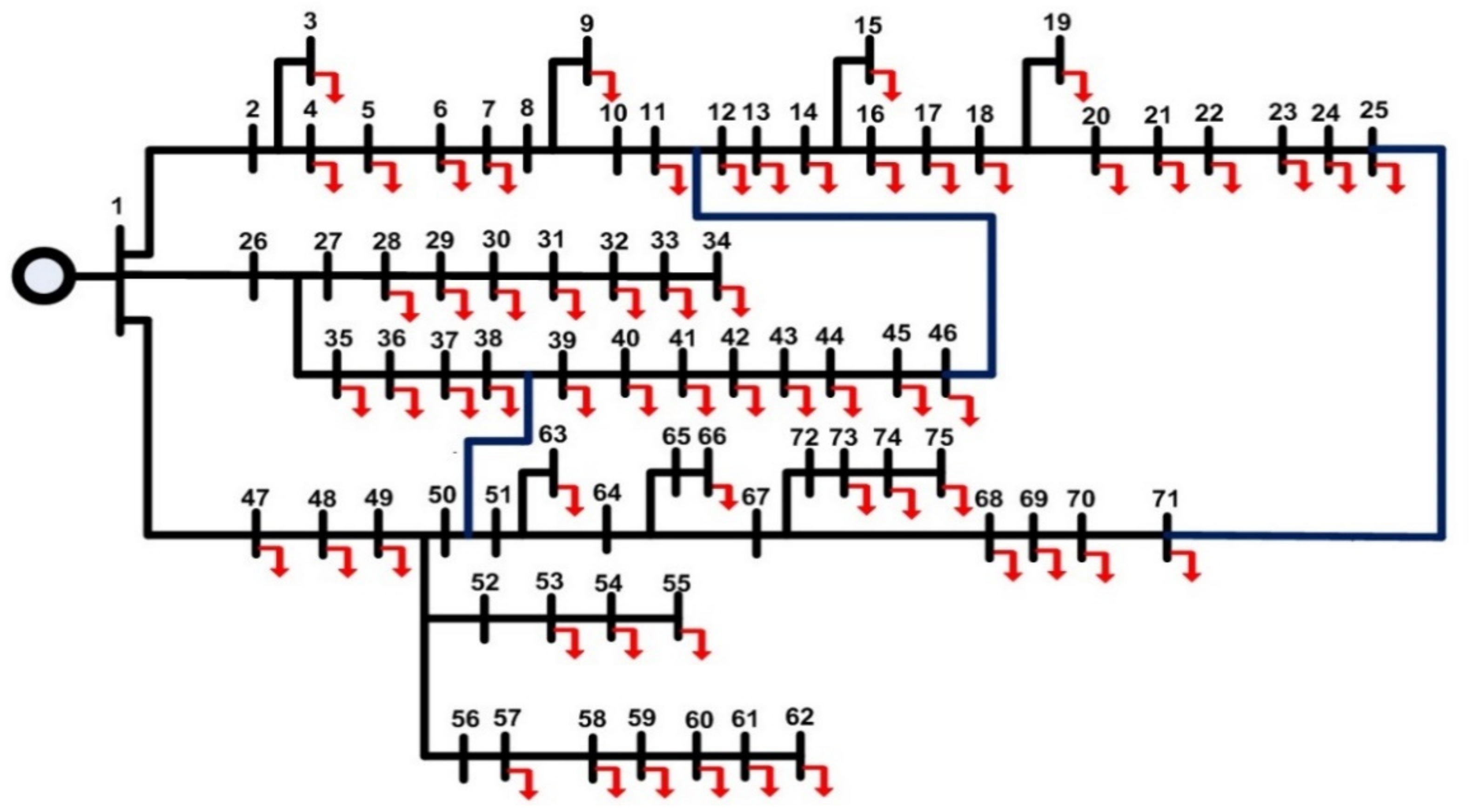
3.2. Mesh-Configured NUST Microgrid for Expansion-Based Study

The other test distribution mechanism is a mesh-configured microgrid (MCMG) and consists of 65 buses/nodes initially. Test MCMG data were taken from an actual system from the National University of Sciences and Technology (NUST), H-12 Campus, Pakistan, to evaluate the performance of the proposed technique in terms of an actual, practical distribution mechanism. The P_LD and Q_LD account for 3950.505 KW and 1913.317 KVAR, under NL (as per data of the year 2020), respectively. The P_Loss and Q_Loss of 60.51 KW and 34.63 KVAR, under NL, without any assets integrated, respectively. The load growth (LG) was applied in two variants with 65 fixed nodes. In the first variant, there are two variations: first, the linear load growth of 1.725% (as per NUST data) was applied in LG1 across 5 years. The P_LD and Q_LD account for 4303.2 KW and 2084.14 KVAR, under LG1 (until 2025), respectively. The P_Loss and Q_Loss account for 64.23 KW and 43.44 KVAR, under LG1, respectively. In the first variant, under the second variation, linear load growth of 2.88% (as per NUST data) was applied in LG2 across another 5 years of the planning horizon. The P_LD and Q_LD account for 4960 KW and 2401 KVAR, under LG2 (until 2030), respectively. The P_Loss and Q_Loss account for 69.01 KW and 53.46 KVAR, under LG2, respectively. The 65-bus MCMG as a second test distribution mechanism is shown in Figure 4. Details of the parameters of both 65- and 75-bus variants of the MCMG are shown in detail in the Appendix of the paper’s Supplementary Materials.

In the second variant of load growth, there are two variations: first with 65 fixed nodes with a respective high percentage across 5 years and later with increased 10 buses expanded to a 75-bus system incorporating new loads in terms of new projects across the following 5 years of the planning horizon, as shown in Figure 5. Under normal load, the values are the same as mentioned before in Section 3.2. For the second LG variant, under the first variation, linear load growth of 7.335% (as per the accommodating future planning data from NUST) was applied in LG1 across 5 years. The P_LD and Q_LD account for 5634.3 KW and 2712.85 KVAR, under LG1 (until the year 2025), respectively. The P_Loss and Q_Loss account for 93.53 KW and 80.43 KVAR, under LG1, respectively. In the second variant, under the second variation, linear load growth of 15.392% (as per accommodating future planning data from NUST) was applied in LG2 across another 5 years of the planning horizon. The P_LD and Q_LD account for 11,527.1 KW and 5550.25 KVAR, under LG2 (until the year 2030), respectively. The P_Loss and Q_Loss account for 205.87 KW and 194.58 KVAR, under LG2, respectively. In total, both load growth horizons correspond to a cumulative 10 years. The 75-bus MCMG as an extended version of the 65-bus MCMG is shown in Figure 5.

The test setup was developed in MATLAB/Simulink R2018a, and numerical values are called in m-files, where the proposed approach was evaluated into achieved results. Initially, the assets were placed on designated locations given by VSIs in previous works in [40,41,42] and proposed as VSI_W in this paper. The base case model was made in Simulink, and the values are called in the m-file, which indicates the weakest nodes as per the respective VSI. Later, the numerical values were obtained from the simulation setup in Simulink and run until the condition where the loop currents across TSs were near zero and voltages across the respective nodes were equal to the optimal sizing of assets considering the termination criteria of 1%. Finally, on termination, the achieved values were called in a program made of m-files (MATLAB 2018a), where the proposed MCSP approach was evaluated with various matrices, shown in Section 3.5.

3.3. Computational Procedure with Cases, Scenarios, and Alternatives for the 33-Bus Active Distribution Network

The computational procedure for the VSI_W-based MCSP approach is the same as the VSI_A and VSI_B counterparts-based approaches (utilized as comparative candidates for validation) followed by LMC reported in [40,41]. Evaluation for alternatives was carried out across assets such as DG (Type 1) and decoupled asset sets REG + D-STATCOM across normal and multiple load growth levels. As per Stage 1 of the proposed MCSP approach, solutions were evaluated in terms of TPE, CPE, EPE, and SPE across normal load (NL). In Stage 2, the normalized values of the above-mentioned individual evaluations and respective combinations (TCPE, ESPE, and OPE) were further evaluated across various MCDM methodologies under NL. In the first part of Stage 2, the evaluations across Stages 1–2 were evaluated with increasing load growth (LG) across a certain planning horizon while keeping the sizing of various assets at the NL level, aiming at respective trade-off solutions. In a later part of Stage 3, the optimal sizing of assets was re-evaluated across Stages 1–2 to arrive at trade-off solutions that suit the upgraded asset sizing across optimal load growth (OLG). The following are alternatives achieved as per Stage 1: Case 1 with DGs operating at 0.9 lagging power factor (LPF) only and Case 2 with an asset set (REG + D-STATCOM) considering an equivalent capacity provided by the respective REG (P only) and D-STATCOM (Q only). These cases and alternatives pertain to evaluations across the mesh-configured 33-bus system

• Case 1: Alternatives = n × DGs only assets operating at 0.90 LPF.
• Case 2: Alternatives = n × asset sets (REG + D-STATCOM) with power equivalent to 0.90 LPF.
• Alternate 1 (A1): 1 × DG [40] or 1 × asset set (REG + D-STATCOM) with VSI_A-LMC [41].
• Alternate 2 (A2): 1 × DG [41] or 1 × asset set (REG + D-STATCOM) with VSI_B-LMC [41].
• Alternate 3 (A3): 2 × DG [40] or 2 × asset sets (REG + D-STATCOM) with VSI_A-LMC [41].
• Alternate 4 (A4): 2 × DG [41] or 2 × asset sets (REG + D-STATCOM) with VSI_B-LMC [41].
• Alternate 5 (A5): 3 × DG [40] or 3 × asset sets (REG + D-STATCOM) with VSI_A-LMC [42].
• Alternate 6 (A6): 3 × DG [40] or 3 × asset sets (REG + D-STATCOM) with VSI_A-LMC [42].
• Alternate 7 (A7): 3 × DG [42] or 3 × asset sets (REG + D-STATCOM) with VSI_B-LMC [42].
• Alternate 8 (A8): 3 × DG [P] or 3 × asset sets (REG + D-STATCOM) with VSI_W-LMC [P].

In Stage 2, all of the above eight alternatives are evaluated across technical (TPE), cost-economic (CPE), environmental (EPE), and social (SPE) criteria, normalized for further performance analysis in two cases across four MCDM methodologies under normal loading conditions of test DNs. The MCDM evaluations from normal loading conditions were evaluated individually across TPE, CPE, EPE, and SPE, as well as collectively across combinations such as TCPE, ESPE, and OPE, respectively.

In Stage 3, the above-mentioned eight alternatives are evaluated in two cases across four MCDM methodologies under normal load (NL), followed by load growth cases across four loading scenarios. The first load growth horizon (LG1) across five years, first optimal load growth horizon (OLG1) across five years, second load growth horizon (LG2) across 10 years, and second optimal load growth horizon (OLG2) across 10 years, respectively. In the NL scenario, the rated load of test DNs is considered, and all the alternatives with respective asset sizing are evaluated. In the LG1 loading scenario, a 7.5% increment in load per annum is considered across a planning horizon of five years, and asset sizing obtained during NL is retained as constant. In OLG1, modified optimal asset sizing is considered across incremented load across five years. OLG1 corresponds to the reinforcement required to maintain a solution after the first planning horizon across 5 years is over. In the LG2 loading scenario, a 7.5% increment in load per annum is considered across a planning horizon of another five years (total of 10 years), and asset sizing obtained during OLG1 is retained as constant. In OLG2, modified optimal asset sizing is considered across incremented load across another five-year planning horizon. OLG2 corresponds to the reinforcement required to maintain a solution after the second planning horizon across another 5 years or 10 years in total is over.

In the above-mentioned two cases (Cases 1–2) with respective designations, each case (C#) was evaluated across the following scenarios (S#) of MCDM evaluations under five load levels (NL, LG1, OLG1, LG2, and OLG2) across the 33-bus test distribution mechanisms, as presented in the nomenclature below.

• Case 1/Scenario 1 (C1/S1): DG only at 0.9 LPF-based evaluations with MCDM under NL.
• Case 1/Scenario 2 (C1/S2): DG at 0.9 LPF-based evaluations with MCDM under LG1.
• Case 1/Scenario 3 (C1/S3): DG at 0.9 LPF-based evaluations with MCDM under OLG1.
• Case 1/Scenario 4 (C1/S4): DG at 0.9 LPF-based evaluations with MCDM under LG2.
• Case 1/Scenario 5 (C1/S5): DG at 0.9 LPF-based evaluations with MCDM under OLG2.
• Case 2/Scenario 1 (C2/S1): REG + D-STATCOM evaluations with MCDM under NL.
• Case 2/Scenario 2 (C2/S2): REG + D-STATCOM evaluations with MCDM under LG1.
• Case 2/Scenario 3 (C2/S3): REG + D-STATCOM evaluations with MCDM under OLG1.
• Case 2/Scenario 4 (C2/S4): REG + D-STATCOM evaluations with MCDM under LG2.
• Case 2/Scenario 5 (C2/S5): REG + D-STATCOM evaluations with MCDM under OLG2.

3.4. Computational Procedure with Cases, Scenarios, and Alternatives for an Actual Mesh-Configured MG

The computational procedure is the same for an actual interconnected configured microgrid and is shown in detail in the following Section 3.5. The computation was applied across four cases with respective scenarios. As per Stage 1, in each respective case and concerned scenarios, VSI_A in [40], VSI_B in [41], and VSI-W in [P] were applied for optimal sizing of assets. Later, LMC was applied for optimal asset sizing. In Stage 2, MCDM methodologies were applied across various multicriteria (TEES) evaluation parameters. In Stage 3, two variants of the load growth with respective variations were applied for a composite evaluation across multiple planning horizons. In all of the above-mentioned cases (Cases 3–6) with respective designations, each case (C#) was evaluated across the following scenarios (S#) of MCDM evaluations under five various load levels across the actual MG test mechanism, as shown in nomenclature below.

• Case 3/Scenario 1 (C3/S1): DG only at 0.9 LPF under NL.
• Case 3/Scenario 2 (C3/S2): DG only at 0.9 LPF under LG1 (Variant 1).
• Case 3/Scenario 3 (C3/S3): DG only at 0.9 LPF under OLG1 (Variant 1).
• Case 3/Scenario 4 (C3/S4): DG only at 0.9 LPF under LG2 (Variant 1).
• Case 3/Scenario 5 (C3/S5): DG only at 0.9 LPF under OLG2 (Variant 1).
• Case 4/Scenario 1 (C4/S1): REG + D-STATCOM under NL.
• Case 4/Scenario 2 (C4/S2): REG + D-STATCOM under LG1 (Variant 1).
• Case 4/Scenario 3 (C4/S3): REG + D-STATCOM under OLG1 (Variant 1).
• Case 4/Scenario 4 (C4/S4): REG + D-STATCOM under LG2 (Variant 1).
• Case 4/Scenario 5 (C4/S5): REG + D-STATCOM under OLG2 (Variant 1).
• Case 5/Scenario 1 (C5/S1): DG only at 0.9 LPF under NL.
• Case 5/Scenario 2 (C5/S2): DG only at 0.9 LPF under LG1 (Variant 2).
• Case 5/Scenario 3 (C5/S3): DG only at 0.9 LPF under OLG1 (Variant 2).
• Case 5/Scenario 4 (C5/S4): DG only at 0.9 LPF under LG2 (Variant 2).
• Case 5/Scenario 5 (C5/S5): DG only at 0.9 LPF under OLG2 (Variant 2).
• Case 6/Scenario 1 (C6/S1): REG + D-STATCOM under NL.
• Case 6/Scenario 2 (C6/S2): REG + D-STATCOM under LG1 (Variant 2).
• Case 6/Scenario 3 (C6/S3): REG + D-STATCOM under OLG1 (Variant 2).
• Case 6/Scenario 4 (C6/S4): REG + D-STATCOM under LG2 (Variant 2).
• Case 6/Scenario 5 (C6/S5): REG + D-STATCOM under OLG2 (Variant 2).

3.5. Performance Evaluation Indicators (PEIs)

The technical and cost-economic indices for performance evaluation are illustrated in

Table 3. Technical performance evaluation (TPE) indices [40,41,42].

S#	TPE Indices		Objective
1	Active Power Loss (PLoss) (KW)	$PLM{C}^{\prime }$= $\min {\displaystyle \sum }_{i=1}^{m_l-1}{\mathrm{P}}_{\mathrm{Loss}}{}^{TDS}+\sum P_{TB}$	Decrease
2	Reactive Power Loss (QLoss) (KVAR)	$QLM{C}^{\prime }$= min${\displaystyle \sum }_{i=1}^{m_l-1}{\mathrm{Q}}_{\mathrm{Loss}}{}^{TDS}+\sum Q_{TB}$	Decrease
3	Active Power Loss Minimization (PLM) (%)	$PLM=\left[\frac{P\_L_{No\_DG}-P\_L_{M\_DG}}{P\_L_{No\_DG}}\right]\times 100$	Increase
4	Reactive Power Loss Minimization (QLM) (%)	$QLM=\left[\frac{Q\_L_{No\_DG}-Q\_L_{M\_DG}}{Q\_L_{No\_DG}}\right]\times 100$	Increase
5	DG Penetration by percentage (DGPP) (%)	$PDG=\left({\displaystyle \sum _{a=1}^M}{P}_{DG}/{\displaystyle \sum _{b=1}^N}{P}_{LD}\right)\times 100$	Increase
6	Voltage Level (P.U)	V = 1.0 (Reference for Ideal)	Increase

and

Table 4. Cost-economic performance evaluation (CPE) indices [40,41,42].

S#	CPE Indices		Objective
1	Cost of Active Power Loss (PLC) Millions USD (M$)	$PLC=\left[P\_L\times E_U\times T_Y \left(8760 h\right)\right]$	Decrease
2	Active Power Loss Saving (PLS) (M$)	$PLS=\frac{PL{C}_{No\_DG}-PL{C}_{M\_DG}}{PL{C}_{No\_DG}}\times 100$	Increase
3	Cost of DG for PDG (CPDG) USD/MWh	$\mathrm{C}\left(P_{DG}\right)$= a ×$P_{DG}{}^2+b\times P_{DG}+c$ where a = 0, b = 20, and c = 0.25	Decrease
4	Cost of DG for QDG (CQDG) USD/MVArh	$\mathrm{C}\left(Q_{DG}\right)$ =$\left[\mathrm{C}\left(S_{DG\_M}\right)-\mathrm{C}\left(\sqrt{\left(S_{DG\_M}{}^2-P_{DG}{}^2\right)}\right)\right]$×k where $S_{D{G}_M}=\frac{P_{D{G}_M}}{\cos \theta }=\frac{1.1\times P_{DG}}{\cos \theta };k=0.5-1$	Decrease
5	Annual Investment Cost (AIC) Million$ (M$)/year (yr.)	$$\begin{gathered} {\displaystyle \sum _{k=1}^{M_{DG}}}A{F}_C\times C{U}_C\times DG{C}_{max} ; \\ \mathrm{where} A{F}_c=\frac{\left(\frac{Ct}{100}\right){\left(1+\frac{Ct}{100}\right)}^T}{{\left(1+\frac{Ct}{100}\right)}^T-1} \end{gathered}$$	Decrease
6	Annual Cost of D-STATCOM (ACD) M$ *(ACD = 0 for DG; For REG, it is added in AIC for D- STATCOM)	$I_C=\left[\frac{{\left(1+C\right)}^{nD}\times C}{{\left(1+C\right)}^{nD}-C}\right] ;$ where ${\mathrm{I}}_{\mathrm{C}}$ = 50 USD/KVAR; C = Rate of Asset Return = 0.1; nD (in yr.) = 5	Decrease

with all relations taken from our previous publications in [40,41,42]. The environmental and social indices for performance evaluation are considered from [34,43,44,45] and are shown in

Table 5. Environment performance evaluation (EPE) indices [43,44].

S#	EPE Indices		Objective
1	CO2 Footprint (kg)	650 g CO2/KWH for oil After conversion = 0.65 kg CO2/KWH For DG only = (DG Generation + Grid Generation) $\times$ 0.65 For DG+DSTAT = (Grid Generation) $\times$ 0.65	Decrease
2	Area Used by Assets (PV) (km2)	Total Area = Total Gen. in KW/(0.18 $\times$ Solar irradiance) Conversion efficiency is 0.18. Solar irradiance for Islamabad is selected as 0.7	Decrease
		50 KVA generator contains a capacity of 20 liters of water For DG only = (DG Generation) $\times$0.4444 $\times$ 0.264172 For DG+DSTAT = (DG Generation) $\times$0.098 $\times$0.264172 where 0.264172 is the conversion factor from liters to gallons, 0.4444 is the water usage factor for the diesel generator, and 0.098 is the water usage factor for solar	Decrease

and

Table 6. Social performance evaluation (SPE) indices [43,44,45].

S#	SPE Indices			Objective
1	Political Acceptance		For DG only, it is 6%: Formula = (Area + Water + CO2) $\times$ 0.06 (values for area, water, and CO2 are from the DG-only case) For DG + DSTATCOM it is 94%: Formula = (Area + Water + CO2) $\times$ 0.94 (values for area, water, and CO2 are from the DG + DSTATCOM case)	Increase.
2	Life Quality	For DG only, it is 15% Formula = (Area + Water + CO2) $\times$ 0.15 (values for area, water, and CO2 are from the DG-only case) For DG + DSTATCOM it is 85% Formula = (Area + Water + CO2) $\times$ 0.85 (values for area, water, and CO2 are from the DG + DSTATCOM case)		Increase
3	Social Awareness	For DG only, it is 35% Formula = (Area + Water + CO2) $\times$ 0.35 (values for area, water, and CO2 are from the DG-only case) For DG + DSTATCOM it is 65% Formula = (Area + Water + CO2) $\times$ 0.65 (values for area, water, and CO2 are from the DG + DSTATCOM case)		Increase

, respectively. All the concerned indices with respective descriptions, relationships, and objectives are illustrated in Table 4, Table 5 and Table 6, respectively. It can be observed that all objectives/criteria are conflicting in nature.

4. Results and Discussion

The proposed MCSP approach was applied as aforementioned in Section 2. The approach was conducted on a 33-bus mesh-configured TDN as an example of an ADN, as shown in Section 3.1. The computational procedure (mentioned in Section 3.3) for the VSI_W (shown in Equation (4))-based MCSP approach is the same as the VSI_A and VSI_B counterparts-based approaches (utilized as comparative candidates for validation) followed by LMC reported in [40,41], as shown in Figure 6. VSI_D is also individually shown in Figure 7.

Weights were allocated in equal proportions (w = 0.333 for each VSI) for initial evaluation and kept equal for VSI_W with respect to Equation (4) in Figure 5. The top three weak buses as potential locations as per Figure 6 correspond to two sets of assets with two variants of VSI_A, first at buses (15, 30, 7) and later at buses (15, 30, 25). For VSI_B, the best locations for asset sitting are for buses (30, 25, 8). For VSI_D, the optimal sitting locations are (15, 32, 30). For the proposed VSI_W, the evaluated locations for asset placements correspond to buses (15, 30, 8). The respective numerical values of VSI_A are (0.7711 @ Bus 15, 0.8106 @ Bus 30, 0.8301 @ Bus 8, and 0.8584 @ Bus 25), normalized VSI_A (VSI_An) are (1.0 @ Bus 15, 0.9513 @ Bus 30, 0.9290 @ Bus 8, and 0.8983 @ Bus 25), VSI_B are (0.0161 @ Bus 30, 0.0140 @ Bus 25, and 0.0127 @ Bus 8), normalized VSI_B (VSI_Bn) are (1.0 @ Bus 30, 0.8696 @ Bus 25, and 0.789 @ Bus 8), VSI_D are (8.46 × 10⁻⁰³ @ Bus 15, 6.92 × 10⁻⁰³ @ Bus 32, and 4.57 × 10⁻⁰³ @ Bus 30), normalized VSI_D (VSI_Dn) are (1.0 @ Bus 15, 0.8176 @ Bus 32, and 0.7207 @ Bus 30), and VSI_W are (0.8935 @ Bus 15, 0.8898 @ Bus 30, and 0.7508 @ Bus 8), respectively. These values show the most critical buses as candidates of asset placement shown in the 33-bus MDN. All values are in per unit (p.u).

The weights in VSI_W were also allocated on the basis of biased weight variations in terms of standard deviation and variance trends to find the sensitivity analysis of change of potential buses/nodes, as shown in Figure 7. The weights on the basis of standard deviation (Std) of the VSI trends for VSI_A, VSI_B, and VSI_D were allocated as 0.00728, 0.37985, and 0.61286, respectively. Weights on the basis of variation (Var) of the VSI trends for VSI_A, VSI_B, and VSI_D were allocated as 0.000105, 0.2777, and 0.7222, respectively. Sensitivity analysis shows that the optimal locations remain the same across all three weighting strategies such as at buses (15, 30, 8) and are considered the final sitting locations for VSI_W-based evaluations.

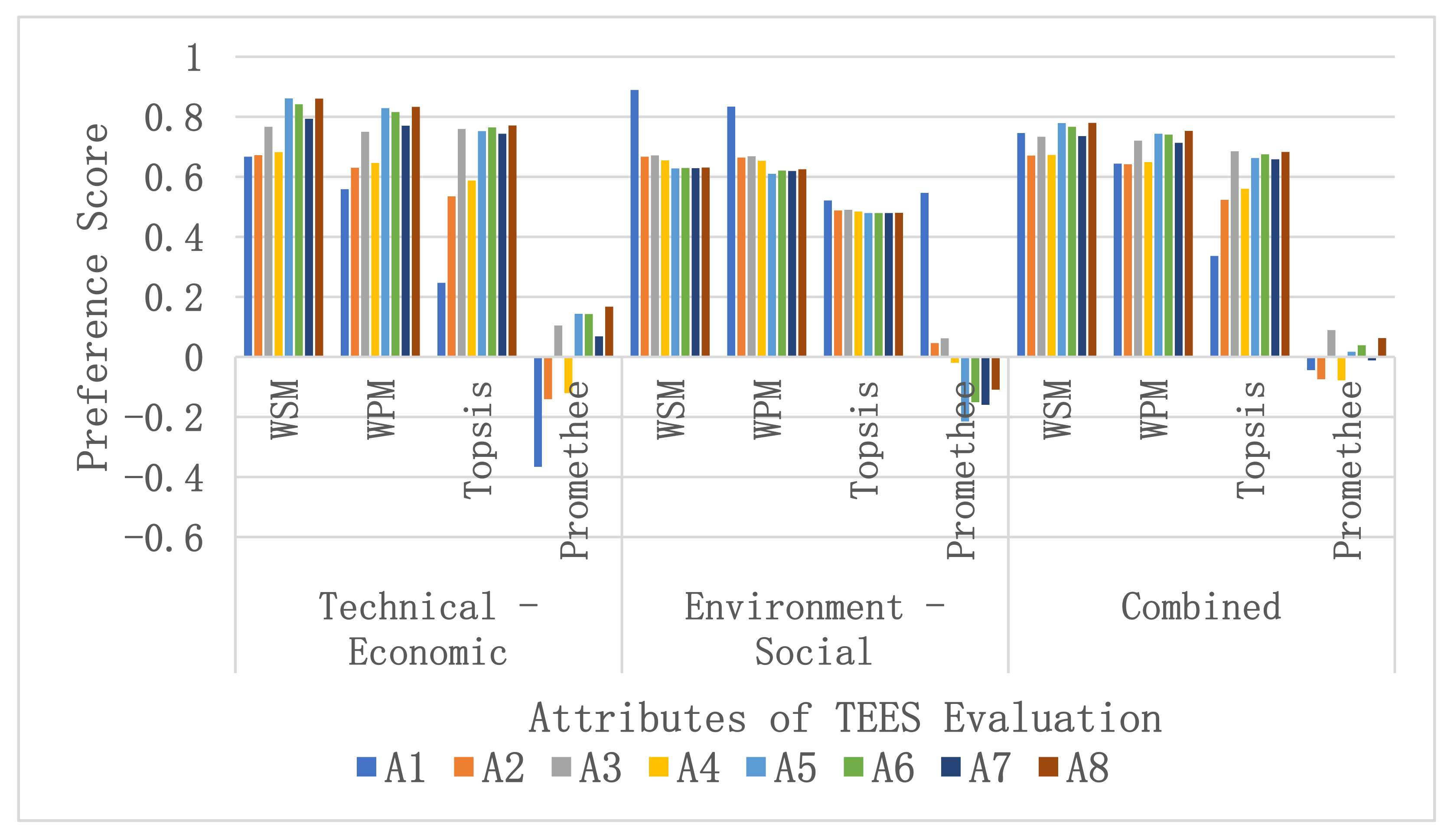
4.1. Case 1: Scenarios 1–5 for DGs Only Operating at 0.90 LPF-Based Placements in the 33-Bus MDN

The evaluation of Case 1 (C1) in terms of scenarios (S1–S5), i.e., C1/S1–S5 for each alternative (total of eight alternatives, i.e., C1/A1–A8) across 0.9 PF lagging aiming at Stage 1 (for sitting and sizing), is shown in

Table 7. DG sitting and sizing at 0.9 LPF for C1/S1–S5 across respective alternatives.

Case (No.)/Alt. (No).	DG Size (KVA) @ Bus Loc. NL (S1)/LG1(S2)	DG Size (KVA) @ Bus Loc. OLG1 (S3)/LG2 (S4)	DG Size (KVA) @ Bus Loc. OLG2(S5)
C1/A1 [40]	DG1: 2013 @ 15	DG1: 2205 @ 15	DG1: 3850 @ 15
C1/A2 [41]	DG1: 2750 @ 30	DG1: 3950 @ 30	DG1: 5730 @ 30
C1/A3 [40]	DG1: 971@15	DG1: 1500 @ 15	DG1: 1800 @ 15
	DG2: 1783 @ 30	DG2: 2300 @ 30	DG2: 4200 @ 30
C1/A4 [41]	DG1: 2357 @ 30	DG1: 3500 @ 30	DG1: 3930 @ 30
	DG2: 540 @ 25	DG2: 590 @ 25	DG2: 2500 @ 25
C1/A5 [40]	DG1: 832.6 @ 15	DG1: 980 @ 15	DG1: 1400 @ 15
	DG2: 1602 @ 30	DG2: 2235 @ 30	DG2: 3450 @ 30
	DG3: 745.1 @ 7	DG3: 1521 @ 7	DG3: 2070 @ 7
C1/A6 [41]	DG1: 894.6 @ 15	DG1: 1147 @ 15	DG1: 1700 @ 15
	DG2: 1386 @ 30	DG2: 2119 @ 30	DG2: 2800 @ 30
	DG3: 822.6 @ 25	DG3: 1272 @ 25	DG3: 2130 @ 25
C1/A7 [42]	DG1: 1957 @ 30	DG1: 2890 @ 30	DG1: 3080 @ 30
	DG2: 500 @ 25	DG2: 590 @ 25	DG2: 2010 @ 25
	DG3: 760 @ 8	DG3: 1090 @ 8	DG3: 1990 @ 8
C1/A8 [P]	DG1: 689.39 @ 15	DG1: 851.88 @ 15	DG1: 1180 @ 15
	DG2: 1602 @ 30	DG2: 2547.72 @ 30	DG2: 3850 @ 30
	DG3: 708.28 @ 8	DG3: 1070.222 @ 8	DG3: 1520 @ 8

. The sizing of assets at respective buses/nodes in alternatives C1/S1–S5/A1–A7 for various assets (DG) in quantities of 1 × DG, 2 × DG, and 3 × DG across NL, LG1, and OLG1 is taken from [40,41,42]. However, they are recalculated across LG2 and OLG2. The values of alternative C1/S1–S5/A8 are evaluated with the proposed VSI_W-LMC for 3 × DG across all planning horizons. A detailed evaluation across each alternative is provided in the Supplementary Materials. In this section, the results of C1/S1–S5/A8 are presented only to avoid repetition and keep the discussion relevant to the proposed results.

Performance evaluation using the TEES criteria was later carried out for each alternative, as aforementioned with respective relationships in Section 3.5. The TPE/CPE evaluations in C1/S1–S5 for the 33-bus MDN are shown in

Table 8. Techno-economic (TPE/CPE) evaluations in C1/S1–S5 for the 33-bus MDN.

S#:	(a) Technical Parameters Evaluation (TPE)						(b) Cost-Economics Parameters Evaluation (CPE)
Case (No.)/Alt. (No).	PLoss (KW)	QLoss (KVAR)	DGPP (%)	PLM (%)	QLM (%)	VMin (P.U)	PLC (M- USD$)	CPDG (USD/ MWh)	CQDG (USD/ MVArh)	AIC (M- USD$)	PLS (M- USD$)
C1/S1/A8	17.393	11.403	68.658	91.307	91.86	0.9915	0.0091	54.244	5.4023	0.5420	0.1018
C1/S2/A8	77.37	43.142	47.822	82.83	85.86	0.9664	0.13129	54.244	5.4023	0.5420	0.8733
C1/S3/A8	36.387	21.197	71.265	91.925	93.05	0.9893	0.01913	80.712	8.0502	0.8077	0.9854
C1/S4/A8	130.58	86.08	49.64	88.24	88.62	0.9528	0.335	80.712	8.0502	0.8077	2.8663
C1/S5/A8	69.38	50.53	72.74	93.75	93.32	0.9858	0.0365	118.15	11.797	1.1835	3.1648

. It is observed from the TPE perspective that C1/S1–S5/A8 had the lowest P_Loss and Q_Loss. On the other hand, it attained the highest P_LM and Q_LM. The V_min is comparatively much better compared to the other counterparts. However, DGPP is comparatively less than C1/S1–S5/S7. From the viewpoint of CPE, C1/S1–S5/A8 was found to achieve the lowest values for PLC, CPDG, CQDG, and AIC, whereas it achieved the highest PLS values in comparison with other alternatives. Likewise, EPE/SPE evaluations in C1/S1–S5 for the 33-bus MDN are shown in

Table 9. Environment-socio (EPE/SPE) evaluations in C1/S1–S5 for the 33-bus MDN.

S#:	(c) Environment Parameters Evaluation (EPE)			(d) Social Parameters Evaluation (SPE)
Case (No.) /Alt. (No).	CO2 (kg)	Land Use (km2)	Water Use (gal)	Political Acceptance	Life Quality	Social Awareness
C1/S1/A8	2204.1630	0.0103	316.9395	151.27	378.17	882.39
C1/S2/A8	2930.4080	0.0103	316.9395	194.84	487.10	1136.58
C1/S3/A8	3200.2295	0.0153	472.3029	220.35	550.88	1285.39
C1/S4/A8	4254.2760	0.0153	472.3029	283.60	708.99	1654.31
C1/S5/A8	4629.1505	0.0225	692.0614	319.27	798.19	1862.43

. In EPE, C1/S1–S5/A8 achieved near to the lowest values in comparison with the 3 × DG scenarios. Likewise, in SPE, it achieves numerical values close to the 3 × DG scenarios. For details, kindly consult the Supplementary Materials section. Complete details of all eight alternatives (A1–A8) across all five scenarios (S1–S5) in Case 1 (C1) in terms of numerical evaluations are documented in Supplementary Materials Sections S.1 and S.1.1.–S.1.5, respectively.

Detailed evaluations of C1/S1 in terms of MCDM methodologies are shown in Figure 8. In Figure 8, it is observed that on the basis of individual evaluations across TCPE, ESPE, and OPE across MCDM methods, Alternative 8 (C1/S1/A8) stands out from the respective counterparts. Details of the respective TEES evaluations, including MCDM methodologies, are shown in Section S.1.1 in the Supplementary Materials. The highest three values are considered for UDS. The first alternative is given the highest score of eight, the second score is seven, and the third is designated as six. Case 1 considering Scenario 1 (C1/S1) results in the top three alternatives in terms of UDS. The respective ranks of alternatives illustrated in Figure 8 across C1/S1 under NL are shown as follows:

• First alternative as per UDS: C1/S1/A8: 72 (First Best).
• Second alternative as per UDS: C1/S1/A7: 62 (Second Best).
• Third alternative as per UDS: C1/S1/A2: 28 (Third Best).

Detailed evaluations of C1/S2 in terms of MCDM methodologies are shown in Figure 9.

In Figure 9, it is observed that on the basis of individual evaluations across TCPE, ESPE, and OPE across MCDM methods, Alternative C1/S2/A8 stands out from the respective counterparts except OPE across TOPSIS C1/S2/A3. Details of respective TEES evaluations are shown in Section S.1.2 in the Supplementary Materials. The highest three values are considered for UDS. The first alternative is given the highest score of eight, the second score is seven, and third is designated as six. C1/S2 results in the top three alternatives in terms of UDS, and the respective ranks of alternatives illustrated in Figure 9 across C1/S2 under LG1 are shown as follows:

• First alternative as per UDS:C1/S2/A8: 63 (First Best).
• Second alternative as per UDS: C1/S2/A6: 48 (Second Best).
• Third alternative as per UDS: C1/S2/A7: 42 (Third Best).

Detailed evaluations of C1/S3 in terms of MCDM methodologies are shown in Figure 10. Details of respective TEES evaluations are shown in Section S.1.3 in the Supplementary Materials. C1/S3 results in the top three alternatives in terms of UDS, and the respective ranks of alternatives illustrated in Figure 10 across C1/S3 under OLG1 are shown below:

• First alternative as per UDS: C1/S3/A8: 70 (First Best).
• Second alternative as per UDS: C1/S3/A6: 49 (Second Best).
• Third alternative as per UDS: C1/S3/A5: 44 (Third Best).

Detailed evaluations of C1/S4 in terms of MCDM methodologies are shown in Figure 11. Details of respective TEES evaluations are shown in Section S.1.4 in the Supplementary Materials. C1/S4 results in the top three alternatives in terms of UDS, and the respective ranks of alternatives illustrated in Figure 11 across C1/S4 under LG2 are shown as follows:

• First alternative as per UDS: C1/S4/A8: 72 (First Best).
• Second alternative as per UDS: C1/S4/A6: 50 (Second Best).
• Third alternative as per UDS: C1/S4/A5: 42 (Third Best).

Detailed evaluations of C1/S5 in terms of MCDM methodologies are shown in Figure 12. Details of respective TEES evaluations are shown in Section S.1.5 in the Supplementary Materials. C1/S5 results in the top three alternatives in terms of UDS, and the respective ranks of alternatives illustrated in Figure 12 across C1/S5 under OLG2 are shown as follows:

• First alternative as per UDS: C1/S5/A8: 60 (First Best).
• Second alternative as per UDS: C1/S5/A5: 58 (Second Best).
• Third alternative as per UDS: C1/S5/A6: 50 (Third Best).

In all the detailed comprehensive TEES evaluations in the respective scenarios (S1–S5) in C1, A8 was found to have permanent presence among the top ranks, hence validating the proposed solution as the best trade-off solution.

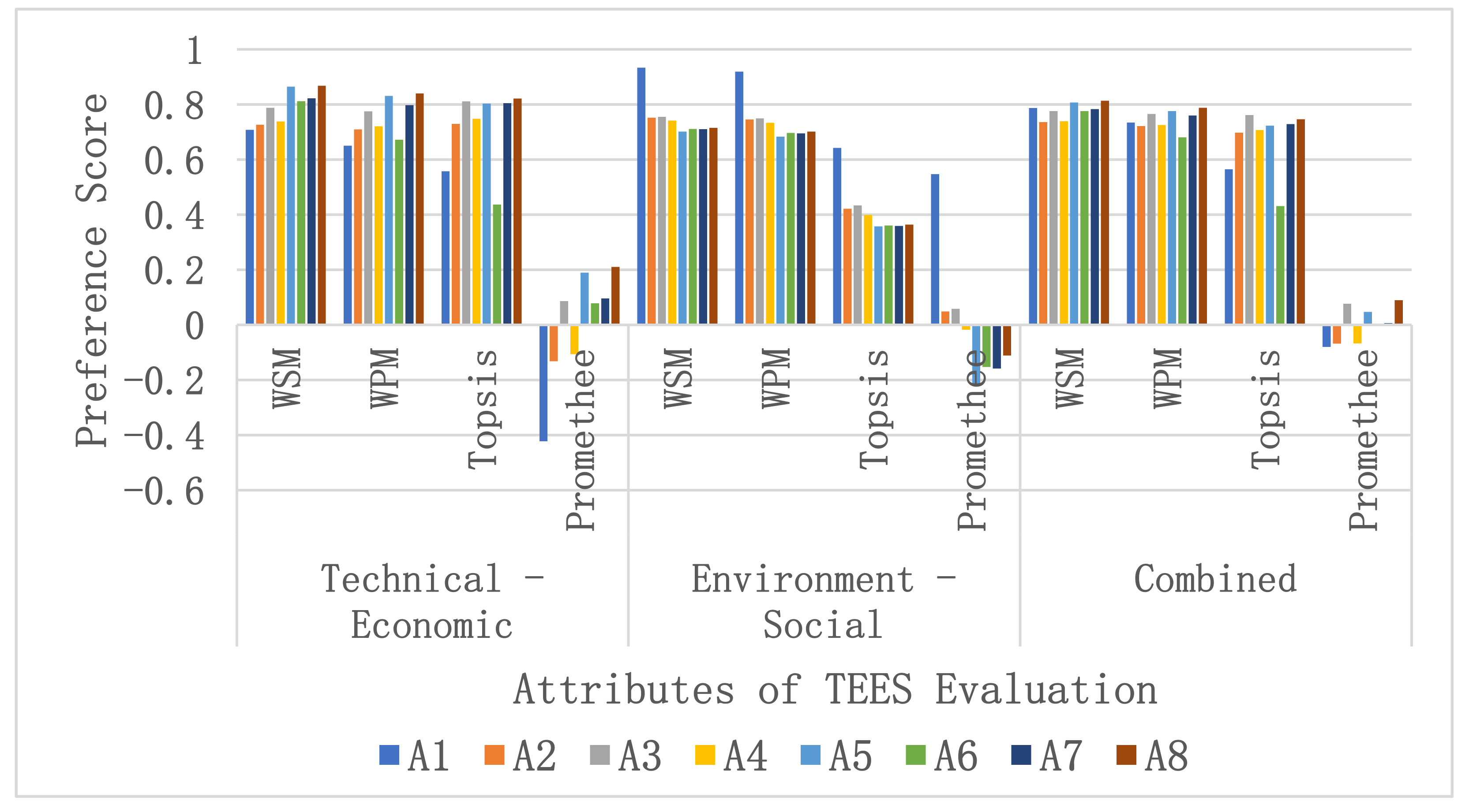
4.2. Case 2: Scenarios 1–5 for REG + D-STATCOM Equal to 0.90 LPF-Based Placements in 33-Bus MDN

The evaluation of Case 2 (C2) in terms of scenarios (S1–S5) across each alternative (total of eight alternatives, i.e., C2/S1–S5/A1–A8) across REG and D-STATCOM, contributes to apparent power equal to that of DG operating at 0.9 PF lagging aiming at Stage 1 (for sitting and sizing) in

Table 10. REG and D-STATCOM set (sitting and sizing) generating power equal to DG at 0.9 LPF for C2/S1–S5 across respective alternatives.

Case (No.)/Alt. (No).	DG Size (KVA) @ Bus Loc. NL (S1)/LG1 (S2)	DG Size (KVA) @ Bus Loc. OLG1 (S3)/LG2 (S4)	DG Size (KVA) @ Bus Loc. OLG2 (S5)
C2/A1 [41]	S1: 1536 + j744 @ 15	S1: 2187 + j1057 @ 15	S1: 3465.9 + j900.61 @ 15
C2/A2 [41]	S1: 2475 + j1199 @ 30	S1: 3558 + j1723 @ 30	S1: 5157 + j2497.65 @ 30
C2/A3 [41]	S1: 869.2 + j421.2 @ 15	S1: 1269 + j622 @ 15	S1: 1621 + j785 @ 15
	S2: 1604 + j777.4 @ 30	S2: 2223 + j1080 @ 30	S2: 3779 + j1830.3 @ 30
C2/A4 [41]	S1: 2121 + j1028 @ 30	S1: 3150 + j1525 @ 30	S1: 3537 + j1713 @ 30
	S2: 486 + j236 @ 25	S2: 531 + j257.1 @ 25	S2: 2250 + j1089.73 @ 25
C2/A5 [42]	S1: 620.5 + j300.5 @15	S1: 882.73 + j427 @15	S1: 1263 + j611.6 @15
	S2: 1442 + j698.3 @ 30	S2: 2011 + j974 @ 30	S2: 3105 + j1504 @ 30
	S3: 637.5 + j308.73 @ 7	S3: 1369 + j663.02 @ 7	S3: 1865 + j903.2 @ 7
C2/A6 [42]	S1: 789 + j380.7 @ 15	S1: 1032 + j500 @ 15	S1: 1529 + j740.6 @ 15
	S2: 1247 + j586.2 @ 30	S2: 1907 + j923.8 @ 30	S2: 2521 + j1221 @ 30
	S3: 739.6 + j372 @ 25	S3: 1145 + j554.5 @ 25	S3: 1917 + j928.5 @ 25
C2/A7 [42]	S1: 1761 + j853 @ 30	S1: 2601 + j1260 @ 30	S1: 2772 + j1342.54 @ 30
	S2: 450 + j218 @ 25	S2: 531 + j257.1 @ 25	S2: 1809 + j876.14 @ 25
	S3: 684 + j331.3 @ 8	S3: 981 + j475.1 @ 8	S3: 1791 + j867.42 @ 8
C2/A8 [P]	S1: 620 + j300.5 @ 15	S1: 766.7 + j371.32 @ 15	S1: 1063.8 + j515.84 @ 15
	S2: 1442 + j698 @ 30	S2: 2293.2 + j1110.6 @ 30	S2: 3466 + j1678.6 @ 30
	S3: 637.5 + j308.8 @ 8	S3: 963.2 + j466.5 @ 8	S3: 1368 + j662.55 @ 8

. The sizing of assets at the respective buses/nodes in alternatives C2/S1–S5/A1–A7 for various assets (DG) at quantities of 1 × asset set (REG and D-STATCOM), 2 × asset set, and 3 × asset set across NL, LG1, and OLG1 is taken from [40,41,42], respectively. However, they are recalculated across LG2 and OLG2. The values of the alternative C2/S1–S5/A8 are evaluated with the proposed VSI_W-LMC for the 3 × asset set (REG and D-STATCOM) across all planning horizons. A detailed evaluation across each alternative is provided in the Supplementary Materials. In this section, the results of C2/S1–S5/A8 are presented only to avoid repetition and keep the discussion relevant to the proposed results.

Performance evaluation across TEES criteria was later carried out across each alternative, as aforementioned with respective relationships in Section 3.5. The TPE/CPE evaluations in C2/S1–S5 for the 33-bus MDN are shown in

Table 11. Techno-economic (TPE/CPE) evaluations in C2/S1–S5 for the 33-bus MDN.

S#:	(a) Technical Parameters Evaluation (TPE)						(b) Cost-Economics Parameters Evaluation (CPE)
Case (No.)/Alt. (No).	PLoss (KW)	QLoss (KVAR)	DGPP (%)	PLM (%)	QLM (%)	VMin (P.U)	PLC (M- USD$)	CPDG (USD/ MWh)	CQDG (USD/ MVArh)	AIC (M- USD$)	PLS (M- USD$)
C2/S1/A8	19.268	11.358	68.651	90.69	91.9	0.9913	0.0101	54.25	5.3713	0.5050	0.1008
C2/S2/A8	78.88	43.48	47.949	82.49	85.75	0.9663	0.13768	54.25	5.5537	0.5051	0.8669
C2/S3/A8	36.9	22.089	71.269	91.811	92.76	0.9892	0.01939	80.708	8.0599	0.7526	0.9852
C2/S4/A8	133.47	87.48	49.64	87.98	88.43	0.9525	0.3512	80.708	8.0599	0.7758	2.8501
C2/S5/A8	74.38	52.78	72.76	93.3	93.02	0.9857	0.0391	118.15	11.849	1.0885	3.1622

. It is observed from the Table 11, from TPE perspective that C2/S1–S5/A8 was found to have the lowest P_Loss and Q_Loss. On the other hand, it attains the highest PLM and QLM. The Vmin is comparatively much better compared to the other counterparts. However, DGPP is comparatively less than C1/S1–S5/S7. From the viewpoint of CPE, C1/S1–S5/A8 was found to achieve the lowest values for PLC, CPDG, CQDG, and AIC, whereas it achieved the highest PLS values in comparison with the other alternatives. The TPE and CPE in C2 were found to be in close agreement with the respective counterparts in C1.

Likewise, EPE/SPE evaluations in C2/S1–S5 for the 33-bus MDN are shown in

Table 12. Environment-socio (EPE/SPE) evaluations in C2/S1–S5 for the 33-bus MDN.

S#:	(c) Environment Parameters Evaluation (EPE)			(d) Social Parameters Evaluation (SPE)
Case (No.) /Alt. (No).	CO2 (kg)	Land Use (km2)	Water Use (gal)	Political Acceptance	Life Quality	Social Awareness
C2/S1/A8	450.3070	0.0214	69.8999	489.01	442.19	338.15
C2/S2/A8	1176.7210	0.0214	69.8999	1171.84	1059.65	810.32
C2/S3/A8	586.6185	0.0319	472.2806	995.40	900.09	688.31
C2/S4/A8	1640.5285	0.0319	472.2806	1986.07	1795.91	1373.35
C2/S5/A8	799.5780	0.0468	692.0614	1402.19	1267.93	969.60

. It is found that a considerable variance and impact of the asset set (REG and D-STATCOM) in numerical values have prolific values in comparison with C1 with the DG-only case, except land use in EPE. It makes sense, as PV-based REG covers a large geographical area compared to the Type 1 synchronous generator operating at 0.9 LPF. However, the evaluated criteria indicate that the overall aimed impacts show a more prominent impact in favor of C2 evaluations rather than C1 across TEES as a whole and EPE and CPE in particular. Details of the evaluation are shown in Section S.2 of the Supplementary Materials.

Detailed evaluations of C2/S1 in terms of MCDM methodologies are shown in Figure 13. Details of respective TEES evaluations, including MCDM methodologies, are shown in Section S.2.1 in the Supplementary Materials. C2/S1 results in the top three alternatives in terms of UDS. The respective ranks of shown in Figure 13 across C2/S1 under NL as follows:

• First alternative as per UDS: C2/S1/A5: 60 (First Best).
• Second alternative as per UDS: C2/S1/A8: 57 (Second Best).
• Third alternative as per UDS: C2/S1/A3: 39 (Third Best).

Comprehensive evaluations of C2/S1 i.e., MCDM methodologies are shown in Figure 13.

Detailed evaluations of C2/S2 in terms of MCDM methodologies are shown in Figure 14. Details of respective TEES evaluations, including MCDM methodologies, are shown in Section S.2.2 in the Supplementary Materials. C2/S2 results in the top three alternatives in terms of UDS. The respective ranks of alternatives illustrated in Figure 14 across C2/S2 under LG1 are shown as follows:

• First alternative as per UDS: C2/S2/A8: 62 (First Best).
• Second alternative as per UDS: C2/S2/A5: 48 (Second Best).
• Third alternative as per UDS: C2/S2/A3: 47 (Third Best).

Detailed evaluations of C2/S3 in terms of MCDM methodologies are shown in Figure 15. Details of respective TEES evaluations, including MCDM methodologies, are shown in Section S.2.3 in the Supplementary Materials. C2/S3 results in the top three alternatives in terms of UDS. The respective ranks of alternatives illustrated in Figure 15 across C2/S3 under OLG1 are shown as follows:

• First alternative as per UDS: C2/S3/A8: 61 (First Best).
• Second alternative as per UDS: C2/S3/A3: 50 (Second Best).
• Third alternative as per UDS: C2/S3/A6: 49 (Third Best).

Detailed evaluations of C2/S4 in terms of MCDM methodologies are shown in Figure 16. Details of respective TEES evaluations, including MCDM methodologies, are shown in Section S.2.4 in the Supplementary Materials. C2/S4 results in the top three alternatives in terms of UDS in Figure 16 across C2/S4 under LG2 are shown as follows:

• First alternative as per UDS: C2/S4/A8: 63 (First Best).
• Second alternative as per UDS: C2/S4/A3: 56 (Second Best).
• Third alternative as per UDS: C2/S4/A5: 41 (Third Best).

Detailed evaluations of C2/S5 in terms of MCDM methodologies are shown in Figure 17. Details of respective TEES evaluations, including MCDM methodologies, are shown in Section S.2.5 in the Supplementary Materials. C2/S4 results in the top three alternatives in terms of UDS in Figure 17 across C2/S5 under OLG2 are shown as follows:

• First alternative as per UDS: C2/S5/A8: 60 (First Best).
• Second alternative as per UDS: C2/S5/A3: 45 (Second Best).
• Third alternative as per UDS: C2/S5/A6: 43 (Third Best).

In all the detailed comprehensive TEES evaluations in the respective scenarios (S1–S5) in C2, A8 was found to have permanent presence among top ranks, except C2/S1. Hence, the comprehensive evaluations validate the proposed solution A8 as the best trade-off solution under the MCSP method.

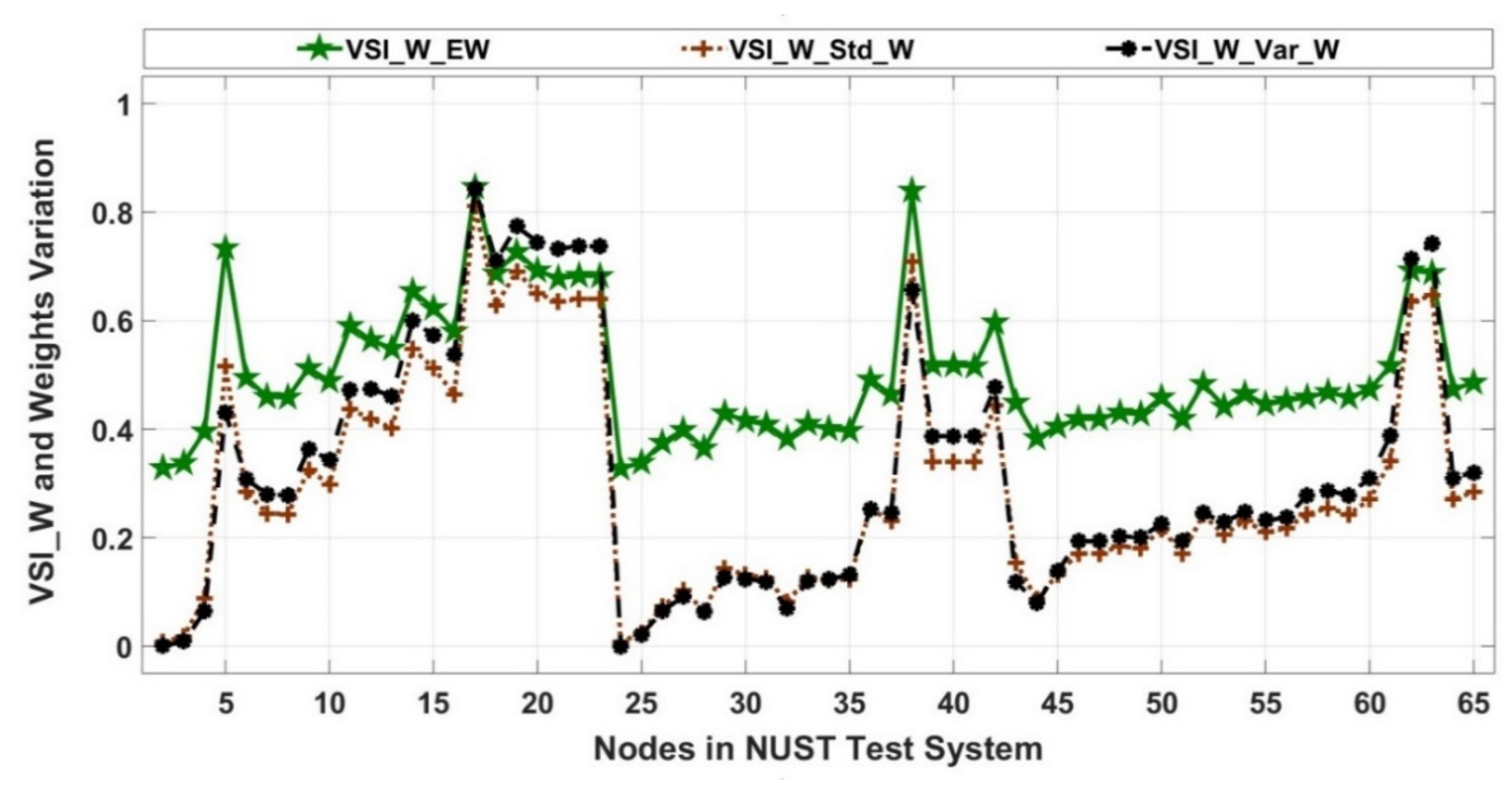
5. Validation and Benchmark Analysis on the NUST Microgrid

The proposed MCSP approach is applied as aforementioned in Section 2. The approach is conducted on the 65-bus and its extended version on the 75-bus mesh-configured MG (MGMC) as an example of modernized ADN under the SG paradigm, as shown in Section 3.2. The computational procedure (mentioned in Section 3.4) for the VSI_W (shown in Equation (4))-based MCSP approach is the same as the VSI_A and VSI_B counterparts-based approaches (utilized as comparative candidates for validation) followed by LMC reported in [40,41], as shown in Figure 18. VSI_W is also individually shown in Figure 19.

The weights allocated in equal proportions (w = 0.333 for each VSI) for initial evaluation were kept equal for VSI_W with respect to Equation (4) in Figure 18. The weights in VSI_W were also allocated on the basis of biased weight variations in terms of standard deviation and variance trends to find the sensitivity analysis of change of potential buses/nodes, as shown in Figure 19. The respective sitting sites for DGs and asset set (REG-D-STATCOM) across VSI_A, VSI_B, and VSI_W are shown as follows:

• Sitting sites in the 65-bus MCMG as per VSI_A:
  • DG1@ 5; DG2 @ 20; DG3 @ 40; DG4 @ 52; DG5 @ 62
• Sitting sites in the 65-bus MCMG as per VSI_B:
  • DG1@ 5; DG2 @ 14; DG3 @ 17; DG4 @ 38; DG5 @ 43
• Sitting sites in the 65-bus MCMG as per VSI_W:
  • DG1@ 5, DG2 @ 17; DG3 @ 38; DG4 @ 42; DG5 @ 62

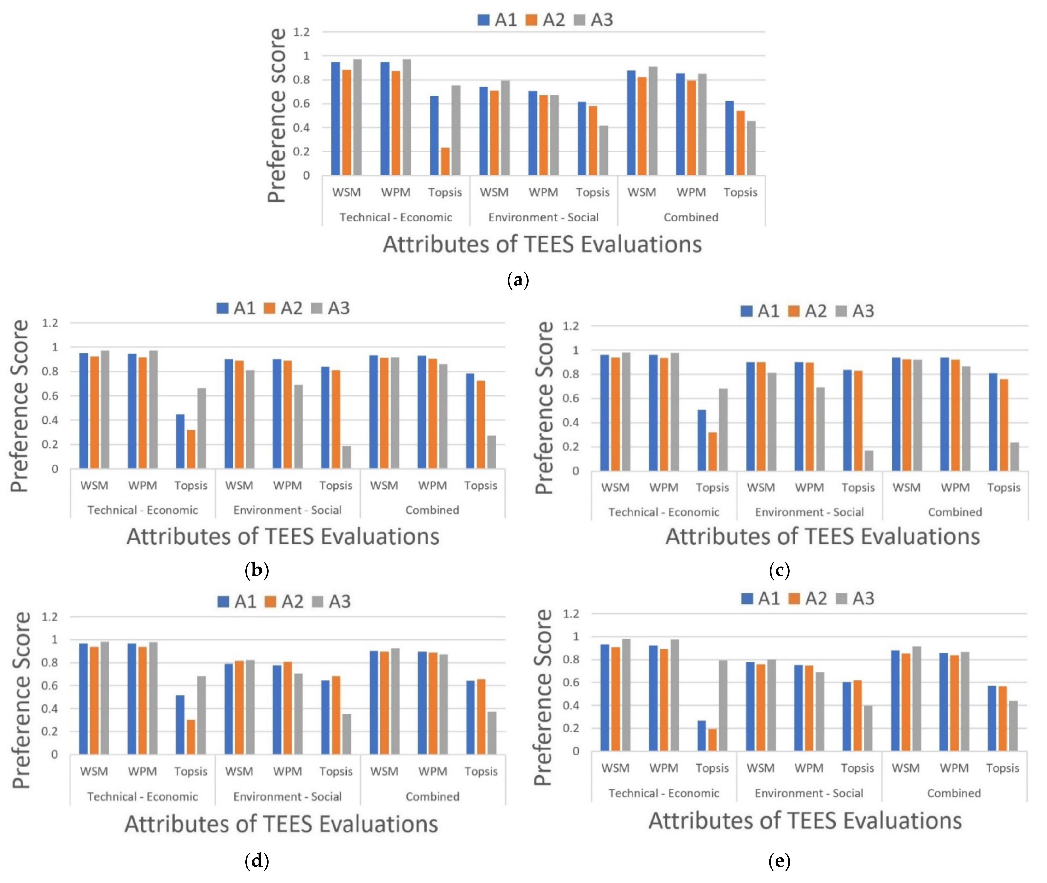
5.1. Case 3: DGs Only Operating at 0.90 LPF-Based Placements in the 65-Bus NUST MCMG

The initial evaluation of Case 3 (C3) in terms of scenarios (S1–S5) for each alternative (A1–A3) across 0.9 PF lagging under various load levels, aiming at Stage 1 (for sitting and sizing), is presented in this section. In C3, the sitting and sizing of DGs only operating at 0.9 LPF are based on VSI_A-LMC [40], VSI_W-LMC [41], and VSI_W-LMC (Stage 1 of the proposed MCSP approach) and were evaluated across all planning horizons (NL, LG1, OLG1, LG2, and OLG2), as shown in

Table 13. DG sitting and sizing at 0.9 LPF for C3/S1–S5 across alternatives in the 65-bus MCMG.

Case (No.)/ Alt. (No).	DG Size (KVA) @ Bus Loc. NL (S1)/LG1 (S2)	DG Size (KVA) @ Bus Loc. OLG1 (S3)/LG2 (S4)	DG Size (KVA) @ Bus Loc. OLG2 (S5)
C3/A1	DG1: 600 @ 05	DG1: 620 @ 05	DG1: 620 @ 05
	DG2: 510 @ 20	DG2: 700 @ 20	DG2: 800 @ 20
	DG3: 870 @ 40	DG3: 950 @ 40	DG3: 1300 @ 40
	DG4: 810 @ 52	DG4: 810 @ 52	DG4: 900 @ 52
	DG5: 460 @ 62	DG5: 460 @ 62	DG5: 460 @ 62
C3/A2	DG1: 300 @ 05	DG1: 300 @ 05	DG1: 350 @ 05
	DG2: 700 @ 14	DG2: 800 @ 14	DG2: 900 @ 14
	DG3: 530 @ 17	DG3: 700 @ 17	DG3: 800 @ 17
	DG4: 950 @ 38	DG4: 1000 @ 38	DG4: 1200 @ 38
	DG5: 950 @ 43	DG5: 950 @ 43	DG5: 950 @ 43
C3/A3	DG1: 400 @ 05	DG1: 470 @ 05	DG1: 520 @ 05
	DG2: 300 @ 17	DG2: 450 @ 17	DG2: 470 @ 17
	DG3: 650 @ 38	DG3: 750 @ 38	DG3: 1050 @ 38
	DG4: 700 @ 42	DG4: 750 @ 42	DG4: 800 @ 42
	DG5: 700 @ 62	DG5: 800 @ 62	DG5: 900 @ 62

. The load growth variant Variant 1 was utilized with a fixed number of nodes/buses across all planning horizons. In this section, the results of C3/S1–S5/A1–A3 are presented in precise detail to avoid repetition and keep the discussion relevant to the proposed results.

A performance evaluation across TEES criteria was later carried out across each alternative, as aforementioned with respective relationships in Section 3.5. The TPE/CPE evaluations in C3/S1–S5 for the 65-bus MVMG are shown in

Table 14. TPE/CPE evaluations in C3/S1–S5 for the 65-bus MDN NUST_MG for DG only @ 0.9 LPF.

S#:	(a) Technical Parameters Evaluation (TPE)						(b) Cost-Economics Parameters Evaluation (CPE)
C3/S1–S5/ Alt (No.)	PLoss (KW)	QLoss (KVAR)	DGPP (%)	PLM (%)	QLM (%)	VMin (P.U)	PLC (M- USD$)	CPDG (USD/ MWh)	CQDG (USD/ MVArh)	AIC (M- USD$)	PLS (M- USD$)
S1/A1	59.62	21.27	74.05	1.65	41.06	0.9993	0.0313	58.75	5.8477	0.5873	0.000526
S1/A2	59.68	36.09	78.16	1.55	38.40	0.9993	0.0314	61.99	6.1775	0.6198	0.000494
S1/A3	59.65	21.79	62.65	1.60	39.62	0.9993	0.0314	49.75	4.9467	0.4968	0.000511
S2/A1	62.9	24.48	67.943	2.07	43.65	0.9992	0.1932	58.75	5.8477	0.5873	0.1968
S2/A2	62.98	25.68	71.74	1.95	40.88	0.9989	0.1934	61.99	6.1775	0.6198	0.1968
S2/A3	62.95	25.22	57.52	1.99	41.94	0.9991	0.1933	49.75	4.9467	0.4968	0.1968
S3/A1	62.88	24.17	74.04	2.1	44.36	0.9992	0.0353	63.97	6.3755	0.6397	0.1968
S3/A2	62.97	25.36	78.43	1.96	41.62	0.9992	0.0331	67.75	6.7537	0.6776	0.1968
S3/A3	62.92	24.75	67.35	2.04	43.02	0.9992	0.0331	58.21	5.7992	0.5818	0.1968
S4/A1	67.24	28.87	64.24	2.56	46	0.9991	0.3899	63.97	6.3755	0.6397	0.4003
S4/A2	67.34	30.31	68.05	2.42	43.3	0.998	0.3905	67.75	6.7537	0.6776	0.4003
S4/A3	67.28	29.5	58.43	2.51	44.82	0.999	0.3901	58.21	5.7992	0.5818	0.4003
S5/A1	67.19	28.04	74.03	2.64	47.55	0.9991	0.0353	73.69	7.348	0.7372	0.4003
S5/A2	67.32	29.82	76.22	2.45	44.22	0.9991	0.0354	75.85	7.5642	0.7589	0.4003
S5/A3	67.25	28.92	67.87	2.55	45.88	0.9991	0.0353	67.57	3.8133	0.648	0.4003

. It is observed from the TPE perspective that C3/S1–S5/A3 was found to have numerical results that are in close approximation to the techniques in previous works and were reapplied for the concerned actual test ADN of the 65-bus MCMG. Nearly the same technical results were achieved from the viewpoint of all technical indices across TPE. The same pattern replicates across the indices of CPE.

Likewise, EPE/SPE evaluations in C3/S1–S5 for the 65-bus MCMG are shown in

Table 15. EPE/SPE evaluations in C3/S1–S5 for the 65-bus MDN NUST_MG for DG only.

S#:	(c) Environment Parameters Evaluation (EPE)			(d) Social Parameters Evaluation (SPE)
C3/S1–S5/ Alt (No.)	CO2 (kg)	Land Use (km2)	Water Use (gal)	Political Acceptance	Life Quality	Social Awareness
S1/A1	2373.872	0.010445	343.3893	163.0363	407.5907	951.0449
S1/A2	2408.276	0.010445	362.4077	166.2462	415.6154	969.7692
S1/A3	2276.807	0.068535	120.6594	154.0572	385.1430	898.6669
S2/A1	2620.059	0.010445	343.3893	244.6629	611.6572	2611.778
S2/A2	2654.841	0.011025	362.4077	246.2855	615.7137	2572.458
S2/A3	2523.554	0.068535	290.5601	237.3341	593.3352	2366.526
S3/A1	2676.024	0.011376	374.0301	250.397	625.9924	1460.649
S3/A2	2716.617	0.012051	396.2184	251.3037	628.2593	1465.938
S3/A3	2614.274	0.073674	340.2195	243.0696	607.6739	1417.906
S4/A1	2957.968	0.011376	374.0301	447.7333	1119.333	2611.778
S4/A2	2998.548	0.012051	396.2184	440.9928	1102.482	2572.458
S4/A3	2896.205	0.073674	340.2195	405.6903	1014.226	2366.526
S5/A1	2887.991	0.013113	374.0301	458.8423	1147.106	2676.580
S5/A2	3085.407	0.0135	396.2184	453.1788	1132.947	2643.543
S5/A3	2996.578	0.07425	340.2195	412.4989	1031.247	2406.244

. In EPE/SPE, C3/S1–S5/A3 achieves near to the lowest values across all planning horizon scenarios in comparison with the other counterparts, designated as C3/S1–S5/A1 and C3/S1–S5/A2, respectively. Hence, comprehensive TEES evaluation across Stage 1 of the proposed MCSP approach testifies its validity.

Detailed evaluations of C3/S1–S5 in terms of MCDM methodologies are shown in Figure 20a–e. Details of respective TEES evaluations, including MCDM methodologies, are shown and summarized numerically in Section S.3 in the Supplementary Materials. C3/S1–S5 results in the top three alternatives in terms of UDS. The respective ranks of alternatives illustrated in Figure 20 across C3/S1–S5 under five load levels were evaluated. It is observed from Figure 20a–e that regarding the alternative C3/S1–S5/A3, which is based on the weighted variant (VSI_W-LMC) of the proposed MCSP approach, the concerned TCPE in all scenarios outperformed the other two alternatives based on previous counterparts (VSI_A and VSI_B-LMC). ESPE and OPE, from the resulting evaluations, were found in close approximation with other methods, thus validate proposed approach.

The MCDM evaluation (including UDS) aiming at finding the ranking of alternatives in C3 in terms of Scenarios 1–5 (S1–S5) for each alternative (total of three alternatives, i.e., C3/S1–S5/A1–A3) across DGs operating at 0.9 PF lagging in the 65-bus mesh-configured microgrid (MCMG), is summarized with relevant details in

Table 16. MCDM evaluations analysis in Case 3 (C3/S1–S5) in terms of UDS for the 65-bus MCMG.

C (#.)/ Alt (No.)	C3/S1 (NL) (UDS)	C3/S2 (LG1) (UDS)	C3/S3 (OLG1) (UDS)	C3/S4 (LG2) (UDS)	C3/S5 (OLG2) (UDS)
C3/A1	22(1)	24(1)	24(1)	24(1)	24(1)
C3/A2	16(3)	15(3)	15(3)	15(3)	15(3)
C3/A3	18(2)	15(2)	15(2)	15(2)	15(2)

, as shown below. The results show that there is no change in ranks in all three alternatives across all load growth horizons. Because the numerical values are in close approximation, the best solution C3/A1 across load horizons suits the decision makers.

5.2. Case 4: REG+DSTATCOM Operating Equal to 0.90 LPF-Based Placements in the 65-Bus NUST MCMG

The initial evaluation of Case 4 (C4) in terms of Scenarios (S1–S5) for each alternative (A1–A3) across asset sets, i.e., REG + D-STATCOM, producing power equal to DG only operating at 0.9 PF lagging under various load levels and aiming at Stage 1 (for sitting and sizing), is shown in

Table 17. Asset set (REG+D-STATCOM) sitting and sizing equal to DG operating at 0.9 LPF for C4/S1–S5 across alternatives in the 65-bus MCMG.

Case (No.)/Alt. (No).	DG Size (KVA) @ Bus Loc. NL (S1)/LG1 (S2)	DG Size (KVA) @ Bus Loc. OLG1 (S3)/LG2 (S4)	DG Size (KVA) @ Bus Loc. OLG2 (S5)
C4/A1	S1: 540 + j262@05	S1: 558 + j270@05	S1: 558 + j270@05
	S2: 459 + j222@20	S2: 630 + j305@20	S2: 720 + j349@20
	S3: 783 + j379@40	S3: 855 + j414@40	S3: 1170 + j567@40
	S4: 729 + j353@52	S4: 729 + j353@52	S4: 810 + j392@52
	S5: 414 + j201@62	S5: 414 + j201@62	S5: 414 + j201@62
C4/A2	S1: 270 + j131@05	S1: 270 + j131@05	S1: 315 + j153@05
	S2: 630 + j305@14	S2: 720 + j349@14	S2: 810 + j392@14
	S3: 477 + j231@17	S3: 630 + j305@17	S3: 720 + j349@17
	S4: 855 + j414@38	S4: 900 + j436@38	S4: 1080 + j523@38
	S5: 855 + j414@43	S5: 855 + j414@43	S5: 855 + j414@43
C4/A3	S1: 360 + j174@05	S1: 423 + j205@05	S1: 468 + j227@05
	S2: 270 + j131@17	S2: 405 + j196@17	S2: 423 + j205@17
	S3: 585 + j283@38	S3: 675 + j327@38	S3: 945 + j458@38
	S4: 630 + j305@42	S4: 675 + j327@42	S4: 720 + j349@42
	S5: 630 + j305@62	S5: 720 + j349@62	S5: 810 + j392@62

. Asset sets (S) are installed in the same sites for C4 as previously placed for DG counterparts in C3.

A performance evaluation across the TEES criteria was later carried out across each alternative in a manner similar to previous cases and with respect to the evaluation relationships mentioned in Section 3.5. TPE/CPE evaluations in C4/S1–S5 for the 65-bus MVMG are shown in

Table 18. TPE/CPE evaluations in C4/S1–S5 for the 65-bus MCMG (NUST_MG) for DG + DSTATCOM.

S#:	(a) Technical Parameters Evaluation (TPE)						(b) Cost-Economics Parameters Evaluation (CPE)
C4/S1–S5/ Alt (No.)	PLoss (KW)	QLoss (KVAR)	DGPP (%)	PLM (%)	QLM (%)	VMin (P.U)	PLC (M- USD$)	CPDG (USD/ MWh)	CQDG (USD/ MVArh)	AIC (M- USD$)	PLS (M- USD$)
S1/A1	59.62	21.27	74.04	1.65	41.06	0.9993	0.0313	58.75	5.8477	0.5712	0.000526
S1/A2	59.68	36.09	78.14	1.55	38.4	0.9993	0.0314	61.99	6.1775	0.6028	0.000494
S1/A3	59.65	21.79	62.64	1.6	39.62	0.9993	0.0314	49.75	4.9467	0.4833	0.00051
S2/A1	62.9	24.48	67.98	2.07	43.65	0.9992	0.1932	58.75	5.8477	0.5712	0.1968
S2/A2	62.98	25.68	71.74	1.95	40.88	0.9989	0.1934	61.99	6.1775	0.6028	0.1968
S2/A3	62.95	25.22	57.51	1.99	41.94	0.9991	0.1933	49.75	4.9467	0.4833	0.1968
S3/A1	62.88	24.17	74.03	2.1	44.36	0.9992	0.0353	63.97	6.3755	0.4657	0.1968
S3/A2	62.97	25.36	78.43	1.96	41.62	0.9992	0.0331	67.75	6.7537	0.4933	0.1968
S3/A3	62.92	24.75	67.35	2.04	43.02	0.9992	0.0331	58.21	5.7992	0.4236	0.1968
S4/A1	67.24	28.87	64.24	2.56	46	0.9991	0.3899	63.97	6.3755	0.4657	0.4003
S4/A2	67.34	30.31	68.05	2.42	43.3	0.998	0.3905	67.75	6.7537	0.4933	0.4003
S4/A3	67.28	29.5	58.43	2.51	44.82	0.999	0.3901	58.21	5.7992	0.4236	0.4003
S5/A1	67.19	28.04	74.02	2.64	47.55	0.9991	0.0353	73.69	7.348	0.3564	0.4003
S5/A2	67.32	29.82	76.21	2.45	44.22	0.9991	0.0354	75.85	7.5642	0.3668	0.4003
S5/A3	67.25	28.92	67.87	2.55	45.88	0.9991	0.0353	67.57	3.8133	0.3215	0.4003

. It is observed from the TPE perspective that C4/S1–S5/A3 was found to have numerical results in close approximation to the techniques in previous works and were reapplied for the concerned actual test ADN of the 65-bus MCMG. Nearly the same technical results were achieved from the viewpoint of all technical indices across TPE when compared individually and with the C3. The same pattern of replicates across the indices of CPE, except for the addition of the D-STATCOM cost (ACD), was added to the annual investment cost (AIC).

Likewise, EPE/SPE evaluations in C4/S1–S5 for the 65-bus MCMG are shown in

Table 19. EPE/SPE evaluations in C4/S1–S5 for the 65-bus MCMG (NUST_MG) for DG+DSTATCOM.

S#:	(c) Environment Parameters Evaluation (EPE)				(d) Social Parameters Evaluation (SPE)
C4/S1–S5/ Alt (No.)	CO2 (kg)	Land Use (km2)	Water Use (gal)	Political Acceptance	Life Quality	Social Awareness
S1/A1	472.6215	0.02321	75.7249	515.4674	466.1142	356.4402
S1/A2	401.726	0.0245	79.9189	452.9248	409.5596	313.1927
S1/A3	668.057	0.1523	26.60805	688.7316	622.7892	476.2505
S2/A1	718.809	0.02321	75.7249	1129.332	1021.205	780.9211
S2/A2	648.2905	0.0245	79.9189	1098.374	993.2102	759.5137
S2/A3	914.8035	0.1523	64.07492	1272.019	1150.23	879.5877
S3/A1	605.124	0.02528	82.4819	1018.426	920.9171	704.2308
S3/A2	522.8665	0.02678	87.37489	1001.343	905.47	692.4182
S3/A3	730.574	0.16372	75.0259	1161.139	1049.966	802.9155
S4/A1	887.068	0.02528	82.4819	1462.768	1322.716	1011.488
S4/A2	804.7975	0.02678	87.37489	1595.603	1442.833	1103.343
S4/A3	1012.505	0.16372	75.0259	2278.533	2060.375	1575.581
S5/A1	501.191	0.02914	95.06388	1247.874	1128.397	862.8915
S5/A2	628.407	0.03	97.85988	1359.943	1229.736	940.3863
S5/A3	808.678	0.165	87.14189	2146.816	1941.27	1484.501

. In EPE/SPE, C4/S1–S5/A3 achieves near to the lowest values across all planning horizon scenarios in comparison with the other counterparts, designated as C4/S1–S5/A1 and C4/S1–S5/A2, respectively. A significant difference in numerical result values was achieved, observed in the C4 comparison with respect to C3 in EPE and SPE. In EPE, it is observed that there is a significant impact on CO₂ emissions reduction and water usage in C4 as a whole rather than a slight increase in land use in C3. From the perspective of SPE, political acceptance and life quality criteria are high, yet social awareness is comparatively low compared to C3 with DG-only assets. Hence, comprehensive TEES evaluation across Stage 1 of the proposed MCSP approach, as well as C3 and C4 evaluation across load growth Variant 1, testifies its validity.

Detailed evaluations of C5/S1–S5 in terms of MCDM methodologies are shown in Figure 21a–e. Details of respective TEES evaluations, including MCDM methodologies, are shown and summarized numerically in Section S.4 in the Supplementary Materials. C4/S1–S5 results in the top three alternatives in terms of UDS in the same manner as conducted in previous case C3/S1–S5 across five load levels. It is observed from Figure 21a–e that regarding the alternative C4/S1–S5/A3, which is based on the proposed MCSP approach, the concerned TCPE in all scenarios outperformed the other two alternatives based on previous counterparts (VSI_A and VSI_B-LMC). ESPE and OPE, from the resulting evaluations, were found in close approximation with other methods.

The MCDM evaluation (including UDS) aiming at finding the ranking of alternatives in C4 in terms of Scenarios 1–5 (S1–S5) for each alternative (total of three alternatives, i.e., C4/S1–S5/A1–A3) across REG + D-STATCOM assets contributing active/reactive power equal to DGs operating at 0.9 PF lagging in the 65-bus mesh-configured microgrid (MCMG), is summarized with relevant details in

Table 20. MCDM evaluations analysis in Case 4 (C4/S1–S5) in terms of UDS for the 65-bus MCMG.

C (#.)/ Alt (No.)	C4/S1 (NL) (UDS)	C4/S2 (LG1) (UDS)	C4/S3 (OLG1) (UDS)	C4/S4 (LG2) (UDS)	C4/S5 (OLG2) (UDS)
C4/A1	21(2)	24(1)	24(1)	18(2)	20(2)
C4/A2	12(3)	14(3)	15(3)	17(3)	13(3)
C4/A3	21(1)	16(2)	15(2)	19(1)	21(1)

. The results show that there is a significant change in ranks in C4/A3 across all load growth horizons. Because the numerical values are in close approximation, the best solution, i.e., C4/A3, ranks highest across most of the load horizons as the preferred solution to opt for.

5.3. Case 5: DGs Operating at 0.90 LPF-Based Placements in Extended 75-Bus NUST MCMG

Performance evaluation across the TEES criteria was later carried out across each alternative with evaluation relationships mentioned in Section 3.5. The increase in load shifted the initial nodes/buses to an increased number of nodes, i.e., the old nodes in the 65-bus MCMG shifted to redesignated nodes in the extended 75-bus MCMG across the first load growth scenario. These cases (C5 and C6) address Variant 2 of the load growth scenario and address the expansion-based planning problem. In C5–C6, similar to C3–C4, the sitting and sizing of DGs only operating at 0.9 LPF are based on VSI_A-LMC [40], VSI_W-LMC [41], and VSI_W-LMC (as Stage 1 of the proposed MCSP approach), evaluated across NL and later expanded to 10 additional nodes in LG1 and OLG1 as per Variant 2 of the load growth. Finally, the nodes were kept constant, as no new nodes were added during LG2 and OLG2, followed by an increase in the load growth as per Variant 2. The DG capacities across all load horizons across C5 are illustrated in

Table 21. DG sitting and sizing at 0.9 LPF for C5/S1–S5 across alternatives in the 75-bus MCMG.

Case (No.)/Alt. (No).	DG Size (KVA) @ Bus Loc. NL/LG1	DG Size (KVA) @ Bus Loc. OLG1/LG2	DG Size (KVA) @ Bus Loc. OLG2
C5/A1	DG1: 600 @ 05	DG1: 620 @ 05	DG1: 700 @ 05
	DG2: 510 @ 20	DG2: 1100 @ 22	DG2: 1500 @ 22
	DG3: 870 @ 40	DG3: 1103 @ 44	DG3: 1800 @ 44
	DG4: 810 @ 52	DG4: 1350 @ 57	DG4: 4770 @ 57
	DG5: 460 @ 62	DG5: 460 @ 70	DG5: 700 @ 70
C5/A2	DG1: 300 @ 05	DG1: 300 @ 05	DG1: 350 @ 05
	DG2: 700 @ 14	DG2: 880 @ 14	DG2: 900 @ 14
	DG3: 530 @ 17	DG3: 1200 @ 18	DG3: 2050 @ 18
	DG4: 950 @ 38	DG4: 1200 @ 42	DG4: 2450 @ 42
	DG5: 950 @ 43	DG5: 1100 @ 47	DG5: 3300 @ 47
C5/A3	DG1: 400 @ 05	DG1: 470 @ 05	DG1: 520 @ 05
	DG2: 300 @ 17	DG2: 700 @ 18	DG2: 860 @ 18
	DG3: 650 @ 38	DG3: 1050 @ 42	DG3: 1800 @ 42
	DG4: 700 @ 42	DG4: 900 @ 46	DG4: 1500 @ 46
	DG5: 700 @ 62	DG5: 1100 @ 70	DG5: 2150 @ 70

. The load growth Variant 2 was utilized with an initially extended (NL to LG1/OLG1) and later fixed (LG2/OLG2) number of nodes/buses across all planning horizons.

TPE/CPE evaluations in C5/S1–S5 for the 75-bus extended MCMG are shown in

Table 22. TPE/CPE evaluations in C5/S1–S5 for the 75-bus MDN NUST_MG for DG only.

S#:	(a) Technical Parameters Evaluation (TPE)						(b) Cost-Economics Parameters Evaluation (CPE)
C5/S1–S5/ Alt (No.)	PLoss (KW)	QLoss (KVAR)	DGPP (%)	PLM (%)	QLM (%)	VMin (P.U)	PLC (M- USD$)	CPDG (USD/ MWh)	CQDG (USD/ MVArh)	AIC (M- USD$)	PLS (M- USD$)
S1/A1	59.62	21.27	74.05	1.65	41.06	0.9993	0.0313	58.75	5.8477	0.5873	0.000526
S1/A2	59.68	36.09	78.16	1.55	38.4	0.9993	0.0314	61.99	6.1775	0.6198	0.000494
S1/A3	59.65	21.79	62.65	1.6	39.62	0.9993	0.0314	49.75	4.9467	0.4968	0.00051
S2/A1	91.09	48.57	51.97	2.61	39.61	0.999	0.2348	77.83	7.7564	0.7787	0.2401
S2/A2	91.30	49.6	54.85	2.38	38.33	0.9985	0.2335	79.45	7.9244	0.795	0.2401
S2/A3	91.23	48.72	43.98	2.46	39.43	0.9985	0.2351	70.45	7.0238	0.7047	0.2401
S3/A1	91.05	45.96	74.09	2.65	42.86	0.9991	0.0479	83.59	8.3386	0.8366	0.2401
S3/A2	91.30	49.41	74.84	2.38	38.57	0.9986	0.048	84.49	8.4287	0.8456	0.2401
S3/A3	91.22	48.53	67.48	2.47	39.66	0.9986	0.0479	76.21	7.6001	0.7625	0.2401
S4/A1	194.6	119.52	36.21	5.48	53.84	0.9963	1.467	159.55	15.9385	1.5991	1.579
S4/A2	197.2	132.12	36.58	4.23	48.97	0.9944	1.4942	152.71	15.2542	1.5305	1.579
S4/A3	196.9	119.34	32.985	4.33	53.9	0.9945	1.4922	117.25	11.7065	1.1745	1.579
S5/A1	194.5	118.67	74.02	5.54	54.16	0.9967	0.1022	170.71	17.0554	1.7112	1.579
S5/A2	197.1	126.02	70.74	4.26	51.32	0.9946	0.1036	164.95	16.479	1.6533	1.579
S5/A3	196.9	119.01	53.39	4.36	54.03	0.9946	0.1035	124.09	12.3908	1.2432	1.579

. It is observed from the TPE perspective that C5/S1–S5/A3 was found to have numerical results that are in close approximation to the techniques in previous works and were reapplied for the concerned actual test ADN of the 75-bus MCMG. Nearly the same technical results were achieved from the viewpoint of all technical indices across TPE. The same pattern of replicates across the indices of CPE, except for the addition of D-STATCOM cost (ACD), was added to annual investment cost (AIC). Likewise, EPE/SPE evaluations in C5/S1–S5 for the 75-bus MCMG are shown in

Table 23. EPE/SPE evaluations in C5/S1–S5 for the 75-bus MDN NUST_MG for DG only.

S#:	(c) Environment Parameters Evaluation (EPE)				(d) Social Parameters Evaluation (SPE)
C5/S1–S5/ Alt (No.)	CO2 (kg)	Land Use (km2)	Water Use (gal)	Political Acceptance	Life Quality	Social Awareness
S1/A1	2373.872	0.010445	343.3893	163.0363	407.5907	951.0449
S1/A2	2408.276	0.085482	362.4077	166.2462	415.6154	969.7692
S1/A3	2276.807	0.252549	290.5601	154.0572	385.143	898.6669
S2/A1	3622.314	0.013851	455.387	244.6629	611.6572	1427.2
S2/A2	3639.779	0.082688	464.8962	246.2855	615.7137	1436.665
S2/A3	3543.222	0.27918	412.0671	237.3341	593.3352	1384.449
S3/A1	3684.07	0.014882	489.1976	250.397	625.9924	1460.649
S3/A2	3693.833	0.081873	494.4805	251.3037	628.2593	1465.938
S3/A3	3604.998	0.284036	445.8777	243.0696	607.6739	1417.906
S4/A1	6527.118	0.028445	935.0754	447.7333	1119.333	2611.778
S4/A2	6454.877	0.077522	894.9252	440.9928	1102.482	2572.458
S4/A3	6074.484	0.241736	686.7785	405.6903	1014.226	2366.526
S5/A1	6646.757	0.030438	1000.583	458.8423	1147.106	2676.58
S5/A2	6586.13	0.07826	966.7728	453.1788	1132.947	2643.543
S5/A3	6147.817	0.236849	726.9286	412.4989	1031.247	2406.244

.

In Table 23, In EPE/SPE, C5/S1–S5/A3 achieves near to the lowest values across all planning horizon scenarios in comparison with other counterparts, designated as C5/S1–S5/A1 and C5/S1–S5/A2, respectively. A significant difference in numerical result values was achieved in C5/S1–S5/A3 in comparison with other counterparts. Hence, comprehensive TEES evaluation across Stage 1 of the proposed MCSP approach testifies its validity. It is also worth mentioning that DG1 placed on Bus 5 remains unchanged. DG2 shifted sites from Bus 20 to Bus 22 due to the addition of two new nodes.

Detailed evaluations of C5/S1–S5 in terms of MCDM methodologies are shown in Figure 22a–d. C5/S1 is the same as C3/S1 under NL. Details of respective TEES evaluations, including MCDM methodologies, are shown and summarized numerically in Section S.5 in the Supplementary Materials. C5/S1–S5 results in the top three alternatives in terms of UDS. The respective ranks of alternatives illustrated in Figure 22 across C5/S1–S5 under five load levels were evaluated. It is observed from Figure 22a–d, the alternative C5/S1–S5/A3, that is based on the weighted variant (VSI_W-LMC) of the proposed MCSP approach, the concerned TCPE in all scenarios were found to outperform other two alternatives based on previous counterparts (VSI_A and VSI_B-LMC). ESPE and OPE, from the resulting evaluations, were found in close approximation with other methods, hence validating the proposed approach.

The MCDM evaluation (including UDS) and aiming at finding the ranking of alternatives in C5 in terms of scenarios (S1–S5) for each alternative (total of three alternatives, i.e., C5/S1–S5/A1–A3) DGs operating at 0.9 PF lagging in the extended 75-bus MCMG are summarized with relevant details are shown in

Table 24. MCDM evaluations analysis in Case 5 (C5/S1–S5) in terms of UDS for extended 75-bus MCMG.

C (#.)/ Alt (No.)	C5/S1 (NL) (UDS)	C5/S2 (LG1) (UDS)	C5/S3 (OLG1) (UDS)	C5/S4 (LG2) (UDS)	C5/S5 (OLG2) (UDS)
C5/A1	23(1)	24(1)	27(1)	24(1)	24(1)
C5/A2	14(3)	14(3)	14(2)	14(3)	14(3)
C5/A3	17(2)	16(2)	13(3)	16(2)	16(2)

. The results show that there is no change of ranks for C5/A1 across all load growth horizons followed by second best rank for alternative C5/A3 (via proposed MCSP approach). Because the numerical values are in close approximation, hence the best solution, i.e., C5/A1, ranks highest across all load horizons and is the preferred solution that decision makers can opt for.

5.4. Case 6: REG+DSTATCOM Operating Equal to 0.90 LPF-Based Placements in the 75-Bus NUST MCMG

The initial evaluation of Case 6 (C6) in terms of scenarios (S1–S5) for each alternative (A1–A3) across the asset sets, i.e., REG + D-STATCOM producing power equal to DG only operating at 0.9 PF lagging under various load levels, aiming at Stage 1 (for sitting and sizing), is shown in

Table 25. Asset set (REG+D-STATCOM) sitting and sizing equal to DG operating at 0.9 LPF for C6/S1–S5 across alternatives in the extended 75-bus MCMG.

Case (No.)/Alt. (No).	DG Size (KVA) @ Bus Loc. NL/LG1	DG Size (KVA) @ Bus Loc. OLG1/LG2	DG Size (KVA) @ Bus Loc. OLG2
C6/A1	S1: 540 + j262 @ 05	S1: 558 + j270 @ 05	S1: 630 + j305 @ 05
	S2: 459 + j222 @ 20	S2: 990 + j480 @ 22	S2: 1350 + j654 @ 22
	S3: 783 + j379 @ 40	S3: 1008 + j448 @ 44	S3: 1620 + j785 @ 44
	S4: 729 + j353 @ 52	S4: 1215 + j589 @ 57	S4: 4293 + j2079 @ 57
	S5: 414 + j201 @ 62	S5: 414 + j201 @ 70	S5: 630 + j305 @ 70
C6/A2	S1: 270 + j131 @ 05	S1: 270 + j131 @ 05	S1: 315 + j153 @ 05
	S2: 630 + j305 @ 14	S2: 792 + j384 @ 14	S2: 810 + j392 @ 14
	S3: 477 + j231 @ 17	S3: 1080 + j523 @ 18	S3: 1845 + j894 @ 18
	S4: 855 + j414 @ 38	S4: 1080 + j523 @ 42	S4: 2295 + j1112 @ 42
	S5: 855 + j414 @ 43	S5: 990 + j480 @ 47	S5: 2970 + j1439 @ 47
C6/A3	S1: 360 + j174 @ 05	S1: 423 + j205 @ 05	S1: 468 + j227 @ 05
	S2: 270 + j131 @ 17	S2: 630 + j305 @ 18	S2: 774 + j375 @ 18
	S3: 585 + j283 @ 38	S3: 945 + j458 @ 42	S3: 1620 + j785 @ 42
	S4: 630 + j305 @ 42	S4: 810 + j393 @ 46	S4: 1395 + j676 @ 46
	S5: 630 + j305 @ 62	S5: 990 + j480 @ 70	S5: 1935 + j937 @70

. Asset sets (S) are installed in the same sites for C6 as previously placed for DG counterparts in C5.

The performance evaluation across TEES criteria is later carried out across each alternative in the manner similar to previous cases and with respect to evaluation relationships mentioned in Section 3.5.

The TPE/CPE evaluations in C6/S1–S5 for the 75-bus extended MCMG are shown in

Table 26. TPE/CPE evaluations in C6/S1–S5 for the 75-bus MDN NUST_MG for DG + DSTATCOM.

S#:	(a) Technical Parameters Evaluation (TPE)						(b) Cost-Economics Parameters Evaluation (CPE)
C6/S1–S5/ Alt (No.)	PLoss (KW)	QLoss (KVAR)	DGPP (%)	PLM (%)	QLM (%)	VMin (P.U)	PLC (M- USD$)	CPDG (USD/ MWh)	CQDG (USD/ MVArh)	AIC (M- USD$)	PLS (M- USD$)
S1/A1	59.62	21.27	74.046	1.65	41.06	0.9993	0.0313	58.75	5.8477	0.5712	0.000526
S1/A2	59.68	36.09	78.13	1.55	38.4	0.9993	0.0314	61.99	6.1775	0.6028	0.000494
S1/A3	59.65	21.79	62.643	1.6	39.62	0.9993	0.0314	49.75	4.9467	0.4833	0.00051
S2/A1	91.09	48.57	51.975	2.61	39.61	0.999	0.2348	77.83	7.7564	0.7575	0.2401
S2/A2	91.3	49.6	54.842	2.38	38.33	0.9985	0.2335	79.45	7.9244	0.7733	0.2401
S2/A3	91.23	48.72	43.97	2.46	39.43	0.9985	0.2351	70.45	7.0238	0.6854	0.2401
S3/A1	91.05	45.96	74.1	2.65	42.86	0.9991	0.0479	83.59	8.3386	0.6091	0.2401
S3/A2	91.3	49.41	74.85	2.38	38.57	0.9986	0.048	84.49	8.4287	0.6156	0.2401
S3/A3	91.22	48.53	67.5	2.47	39.66	0.9986	0.0479	76.21	7.6001	0.5551	0.2401
S4/A1	194.58	119.52	36.215	5.48	53.84	0.9963	1.467	159.55	15.9385	1.1642	1.579
S4/A2	197.16	132.12	36.584	4.23	48.97	0.9944	1.4942	152.71	15.2542	1.1142	1.579
S4/A3	196.95	119.34	33.0	4.33	53.9	0.9945	1.4922	117.25	11.7065	0.8551	1.579
S5/A1	194.47	118.67	74.02	5.54	54.16	0.9967	0.1022	170.71	17.0554	0.8272	1.579
S5/A2	197.1	126.02	71.53	4.26	51.32	0.9946	0.1036	164.95	16.479	0.7992	1.579
S5/A3	196.9	119.01	53.78	4.36	54.03	0.9946	0.1035	124.09	12.3908	0.6009	1.579

. It is observed from the TPE perspective that C6/S1–S5/A3 has numerical results that are in close approximation to the techniques in previous works. Nearly the same technical results were achieved from the viewpoint of all technical indices across TPE when compared individually and with the C5. The same pattern replicates across the indices of CPE, except for the addition of ACD, is added to AIC. Likewise, EPE/SPE evaluations in C6/S1–S5 for extended 75-bus MCMG are shown in

Table 27. EPE/SPE evaluations in C6/S1–S5 for the 75-bus MDN NUST_MG for DG+DSTATCOM.

S#:	(c) Environment Parameters Evaluation (EPE)				(d) Social Parameters Evaluation (SPE)
C6/S1–S5/ Alt (No.)	CO2 (kg)	Land Use (km2)	Water Use (gal)	Political Acceptance	Life Quality	Social Awareness
S1/A1	472.6215	0.02321	75.7249	515.4674	466.1142	356.4402
S1/A2	401.726	0.18996	79.9189	452.9248	409.5596	313.1927
S1/A3	668.057	0.56122	64.07492	688.7316	622.7892	476.2505
S2/A1	1100.964	0.03078	100.4229	1129.332	1021.205	780.9211
S2/A2	1065.779	0.18375	102.5199	1098.374	993.2102	759.5137
S2/A3	1261.722	0.6204	90.86988	1272.019	1150.23	879.5877
S3/A1	975.52	0.03307	107.8789	1018.426	920.9171	704.2308
S3/A2	956.033	0.18194	109.0439	1001.343	905.47	692.4182
S3/A3	1136.298	0.63119	98.32588	1161.139	1049.966	802.9155
S4/A1	1349.868	0.06321	206.2047	1462.768	1322.716	1011.488
S4/A2	1499.927	0.17227	197.3507	1595.603	1442.833	1103.343
S4/A3	2271.984	0.53719	151.4498	2278.533	2060.375	1575.581
S5/A1	1106.807	0.06764	220.6507	1247.874	1128.397	862.8915
S5/A2	1233.38	0.17391	213.1947	1359.943	1229.736	940.3863
S5/A3	2123.017	0.52633	160.3038	2146.816	1941.27	1484.501

.

In Table 27, it is shown that from the perspective of EPE/SPE, C4/S1–S5/A3 achieves near to the lowest values across all planning horizon scenarios in comparison with other counterparts, designated as C4/S1–S5/A1 and C4/S1–S5/A2, respectively. Hence, comprehensive TEES evaluation across Stage 1 of the proposed MCSP approach, as well as C3 and C4 evaluation across load growth Variant 2, testifies its validity.

Detailed evaluations of C6/S1–S5 in terms of MCDM methodologies are shown in Figure 23a–d. C6/S1 is the same as C4/S1 under NL. Details of respective TEES evaluations, including MCDM methodologies, are shown and summarized numerically in Section S.6 in the Supplementary Materials. C6/S1–S5 results in the top three alternatives in terms of UDS. The respective ranks of alternatives illustrated in Figure 23 across C6/S1–S5 under five load levels were evaluated. It is observed from Figure 23a–d, the alternative C5/S1–S5/A3, that is based on the weighted variant (VSI_W-LMC) of the proposed MCSP approach, the concerned TCPE in all scenarios were found to outperform other two alternatives based on previous counterparts. ESPE and OPE, from the resulting evaluations, were found in close approximation with other methods, validating the proposed approach.

The MCDM evaluation (including UDS) aiming at finding the ranking of alternatives in C6 across five scenarios (S1–S5) for each alternative (total of three alternatives, i.e., C6/S1–S5/A1–A3) across REG+D-STATCOM assets contributing active/reactive power equal to DGs operating at 0.9 PF lagging in the extended 75-bus MCMG.

The overall results of C6/S1–S5/A1–A3 are summarized with relevant details as shown in

Table 28. MCDM evaluations analysis in Case 6 (C4/S1–S5) in terms of UDS for the 75-bus MCMG.

C (#.)/ Alt (No.)	C6/S1 (NL) (UDS)	C6/S2 (LG1) (UDS)	C6/S3 (OLG1) (UDS)	C6/S4 (LG2) (UDS)	C6/S5 (OLG2) (UDS)
C6/A1	22(1)	24(1)	24(1)	22(1)	22(1)
C6/A2	11(3)	13(3)	13(3)	12(3)	11(3)
C6/A3	21(2)	17(2)	17(2)	20(2)	21(2)

. The results show that the order of the alternative ranks across all load growth horizons follows the same pattern, as shown in the previous case (C5). Because the numerical values are in close approximation, the best solution, i.e., C6/A1, ranks highest across all load horizons and is the preferred solution to opt for.

5.5. Comparison with Other Reported Works for Further Validation

The evaluation comparison of C1/S1 under NL for best alternative in terms of various performance is shown in

Table 29. Comparisons of results with C1/S1 under NL for the 33-bus MDN (DG@LPF = 0.90).

Performance Indicators	[46]	[46]	[47]	[41]	[P]
DG Size (KVA) @DG Site (Bus)	773 @ 14 378 @ 25 847 @ 30	700 @ 15 430 @ 18 870 @ 28	2074.56 @ 6 615.25 @15	1957 @ 30 500 @ 25 760 @ 8	DG1: 689.39 @ 15 DG2: 1602 @ 30 DG3: 708.28 @ 8
PLoss (KW)	28.83	39.76	65.8435	18.870	17.393
QLoss (KVAR)	-	-	51.94	13.327	11.403
PLM (%)	86.33	81.15	68.8	91.06	91.307
QLM (%)	-	-	63.7	90.68	91.860
DG Capacity (KVA)	1998	2000	2689.81	3217	2999.67
DGPP (%)	45.73	45.77	61.56	73.63	68.658
VMin (P.U)	0.9756	0.9796	0.9757	0.9857	0.9915
PLC (Million-$)	-	-	0.03461	0.00992	0.0091
PLS (Million-$)	-	-	0.07629	0.1010	0.1018
CPDG (USD/MWh)	-	-	-	58.156	54.244
CQDG (USD/MVArh)	-	-	-	5.7938	5.4023
AIC (Million-$)	-	-	-	0.5813	0.5420

Note: The outperformed results in the comparative study are shown in bold text.

. To keep the discussion relevant, the comparison is only conducted across respective NL scenarios. The achieved results are compared with the multi-objective hybrid GA and the TOPSIS approach in [46], the multi-objective centric hybrid sensitivity-based approach in [47], and the VSI-based approach in [41]. The proposed approach outperforms the other techniques across most of the performance indicators.

The best-achieved alternatives in C3_NL are compared in

Table 30. Comparisons of results with C2/S1 under NL for the 33-bus MDN (REG + D-STATCOM@LPF = 0.9).

Performance Indicators	[48]	[49]	[50]	[40]	[P]
DG (KW) @ Bus No. D-STATCOM (KVAR) @ Bus No.	1316 @ 9 740 @ 10	2491 @ 6 1230 @30	750 @ 14 420 @ 14	620.5 @ 15 300 @ 15	620 @ 15 300.5 @ 15
			1100 @ 24 460 @ 24	1442 @ 30 698.3 @ 30	1442 @ 30 698 @ 30
			1000 @ 8 970 @ 8	637.5 @ 7 308.73 @ 7	637.5 @ 8 308.8 @ 8
PLoss (KW)	48.73	58	15.07	19.40	19.268
QLoss (KVAR)	-	-	-	11.09	11.358
PLM (%)	76.9	72.51	92.56	90.63	90.69
QLM (%)	-	-	-	92.09	91.90
DG Capacity (KW)	1316	2491	2460	2700	2700
D-STATCOM Capacity (KVAR)	740	1230	1600	1307.03	1307.30
DGPP (%)	34.56	67	67.2	68.651	68.651
VMin (P.U)	-	-	0.9584	0.9900	0.9913
PLC (Million-$)	-	-	-	0.0102	0.0101
PLS (Million-$)	-	-	-	0.1007	0.1008
CPDG (USD/MWh)	-	50.1	-	54.25	54.25
CQDG (USD/MVArh)	-	5.2	-	5.3593	5.3713
AIC +ACD (Million-$)	-	-	-	0.52708	0.5050

Note: The outperformed results in the comparative study are shown in bold text.

with well-established approaches such as the hybrid fuzzy ant colony optimization approach in [48], sensitivity-based approach in [49], multiple attribute decision-making (MCDM) methods such as TOPSIS and PROMETHEE in [50], and VSI-based IDMP approach in [40]. It is found that A8 in the proposed approach among the findings of the other solutions is in close agreement and outperforms in several aspects of the reported works, hence validating the proposed approach under NL.

6. Conclusions

Modern distribution mechanisms such as active distribution networks and microgrids are considered to be reliable in nature and interconnected in topology, aiming at better performance across various criteria of conflicting genres, within the smart grid paradigm. This research work offers a multiple-criteria-based sustainable planning (MCSP) approach that aims to serve as a tool for modern distribution mechanisms in terms of trade-off solutions among practical planning problems with conflicting criteria across multiple planning horizons. The proposed MCSP approach is a multistage approach that aims at the sitting and sizing of various assets with a weighted voltage stability index (VSI_W) and loss minimization condition (LMC) in the stage 1. Later, an evaluation of alternatives (solutions) was carried out across four dimensions (technical, economic, environmental, and social) of performance metrics. The assets considered in the evaluations included distributed generation (DG), renewable DGs, i.e., photovoltaic (PV), wind, and distributed static compensator (D-STATCOM) units. In the stage 2, various multi-criteria decision-making methodologies followed by unanimous decision-making scores were applied to ascertain the best trade-off among the available solutions in terms of overall (TEES) performance evaluations (OPE). In the stage 3, the alternatives were evaluated across multiple load growth horizons of 5 years each. The proposed MCSP approach was evaluated across a mesh-configured 33-bus active distribution network (ADN) and an actual NUST microgrid (MCMG), with one and two variants of load growth, respectively. On the whole, six cases were evaluated across normal load, load growth, and optimal load growth. Detailed performance analysis was applied across the mesh-configured 33-bus test distribution network in terms of two cases of DG operating at 0.9 LPF and REG-D-STATCOM sets as respective asset optimization cases. Likewise, four cases of the proposed MCSP approach were applied across two variants of load growth across an actual 65-bus mesh-configured microgrid and an extended 75-bus variant of a mesh-configured microgrid situated in NUST University, Pakistan. The achieved results across all cases after comparison with reported and extended studies were in close approximation, particularly in the performance evaluation among conflicting criteria of various genres across the multiple planning horizons with respective load growth cases. It also reduces the time required for evaluations and sensitivity analysis. Moreover, the proposed approach provides a wide range of trade-off solutions across various performance metrics with respective validity. The proposed MCSP approach can serve as an important planning tool for interconnected distribution mechanisms for researchers and planning engineers.

References

1. Keane, A.; Ochoa, L.; Borges, C.L.T.; Ault, G.W.; Alarcon-Rodriguez, A.; Currie, R.A.F.; Pilo, F.; Dent, C.; Harrison, G.P. State-of-the-Art Techniques and Challenges Ahead for Distributed Generation Planning and Optimization. IEEE Trans. Power Syst. 2012, 28, 1493–1502. [Google Scholar] [CrossRef] [Green Version]
2. Evangelopoulos, V.A.; Georgilakis, P.; Hatziargyriou, N.D. Optimal operation of smart distribution networks: A review of models, methods and future research. Electr. Power Syst. Res. 2016, 140, 95–106. [Google Scholar] [CrossRef]
3. Li, R.; Wang, W.; Chen, Z.; Jiang, J.; Zhang, W. A Review of Optimal Planning Active Distribution System: Models, Methods, and Future Researches. Energies 2017, 10, 1715. [Google Scholar] [CrossRef] [Green Version]
4. Kazmi, S.A.A.; Shahzad, M.K.; Shin, D.R. Multi-Objective Planning Techniques in Distribution Networks: A Composite Review. Energies 2017, 10, 208. [Google Scholar] [CrossRef] [Green Version]
5. Kazmi, S.A.A.; Shahzaad, M.K.; Shin, D.R. Voltage Stability Index for Distribution Network connected in Loop Configuration. IETE J. Res. 2017, 63, 1–13. [Google Scholar] [CrossRef]
6. Kumar, P.; Gupta, N.; Niazi, K.R.; Swarnkar, A. A Circuit Theory-Based Loss Allocation Method for Active Distribution Systems. IEEE Trans. Smart Grid 2017, 10, 1005–1012. [Google Scholar] [CrossRef]
7. Che, L.; Zhang, X.; Shahidehpour, M.; AlAbdulwahab, A.; Al-Turki, Y. Optimal Planning of Loop-Based Microgrid Topology. IEEE Trans. Smart Grid 2016, 8, 1771–1781. [Google Scholar] [CrossRef]
8. Cortes, C.A.; Contreras, S.F.; Shahidehpour, M. Microgrid Topology Planning for Enhancing the Reliability of Active Distribution Networks. IEEE Trans. Smart Grid 2017, 9, 6369–6377. [Google Scholar]
9. Arefifar, S.A.; Mohamed, Y.A.R.I.; El-Fouly, T. Optimized Multiple Microgrid-Based Clustering of Active Distribution Systems Considering Communication and Control Requirements 2015. IEEE Trans. Ind. Electron. 2015, 62, 711–723. [Google Scholar] [CrossRef]
10. Kazmi, S.A.A.; Shahzad, M.K.; Khan, A.Z.; Shin, D.R. Smart Distribution Networks: A Review of Modern Distribution Concepts from a Planning Perspective. Energies 2017, 10, 501. [Google Scholar] [CrossRef]
11. Mahmoud, P.H.A.; Phung, D.H.; Vigna, K.R. A review of the optimal allocation of distributed generation: Objectives, constraints, methods, and algorithms. Renew. Sustain. Energy Rev. 2017, 75, 293–312. [Google Scholar]
12. Prakash, P.; Khatod, D.K. Optimal sizing and sitting techniques for distributed generation in distribution systems: A review. Renew. Sustain. Energy Rev. 2016, 57, 111–130. [Google Scholar] [CrossRef]
13. Sirjani, R.; Jordehi, A.R. Optimal placement and sizing of distribution static compensator (D-STATCOM) in electric distribution networks: A review. Renew. Sustain. Energy Rev. 2017, 77, 688–694. [Google Scholar] [CrossRef]
14. Kumar, A.B.; Sah, A.R.; Singh, Y.; Deng, X.; He, P.; Kumar, R.C. BansalA review of multi criteria decision making (MCDM) towards sustainable renewable energy development. Renew. Sust. Energy Rev. 2017, 69, 596–609. [Google Scholar] [CrossRef]
15. Stojcic, M.; Zavadskas, E.K.; Pamucar, D.; Stevic, Z.; Mardani, A. Application of MCDM Methods in Sustainability Engineering: A Literature Review 2008–2018. Symmetry 2019, 11, 350. [Google Scholar] [CrossRef] [Green Version]
16. Sharma, A.K.; Murty, V.V.S.N. Analysis of Mesh Distribution Systems Considering Load Models and Load Growth Impact with Loops on System Performance. J. Inst. Eng. Ser. B 2014, 95, 295–318. [Google Scholar] [CrossRef]
17. Alvarez-Herault, M.-C.; N’Doye, N.; Gandioli, C.; Hadjsaid, N.; Tixador, P. Meshed distribution network vs. reinforcement to increase the distributed generation connection. Sustain. Energy Grids Netw. 2015, 1, 20–27. [Google Scholar] [CrossRef]
18. Chen, T.H.; Lin, E.H.; Yang, N.C.; Hsieh, T.Y. Multi-objective optimization for upgrading primary feeders with distributed generators from normally closed loop to mesh arrangement. Int. J. Elect. Pow. Energy Syst. 2013, 45, 413–419. [Google Scholar] [CrossRef]
19. Sun, C.; Mi, Z.; Ren, H.; Jing, Z.; Lu, J.; Watts, D. Multi-Dimensional Indexes for the Sustainability Evaluation of an Active Distribution Network. Energies 2019, 12, 369. [Google Scholar] [CrossRef] [Green Version]
20. Das, B.K.; Hoque, N.; Mandal, S.; Pal, T.K.; Raihan, M.A. A techno-economic feasibility of a stand-alone hybrid power generation for remote area application in Bangladesh. Energy 2017, 134, 775–788. [Google Scholar] [CrossRef]
21. Al-Sharafi, A.; Sahin, A.Z.; Ayar, T.; Yilbas, B.S. Techno-economic analysis and optimization of solar and wind energy systems for power generation and hydrogen production in Saudi Arabia. Renew. Sustain. Energy Rev. 2017, 69, 33–49. [Google Scholar] [CrossRef]
22. Shahzad, M.K.; Zahid, A.; Rashid, T.U.; Rehan, M.A.; Ali, M.; Ahmad, M. Techno-economic feasibility analysis of a solar-biomass off grid system for the electrification of remote rural areas in Pakistan using HOMER software. Int. J. Renew. Energy 2017, 106, 264–273. [Google Scholar] [CrossRef]
23. Das, M.; Singh, M.A.K.; Biswas, A. Techno-economic optimization of an off-grid hybrid renewable energy system using metaheuristic optimization approaches—Case of a radio transmitter station in India. Int. J. Energy Convers. Manag. 2019, 185, 339–352. [Google Scholar] [CrossRef]
24. Duman, A.C.; Guler, O. Techno-economic analysis of off-grid PV/wind/fuel cell hybrid system combinations with a comparison of regularly and seasonally occupied households. Int. J. Sustain. Cities Soc. 2018, 42, 107–126. [Google Scholar] [CrossRef]
25. Hosseinalizadeh, R.; Rafiei, E.S.; Alavijeh, A.S.; Ghaderi, S.F. Economic analysis of small wind turbines in residential energy sector in Iran. Sustain. Energy. Technol. Assess. 2017, 20, 58–71. [Google Scholar] [CrossRef]
26. Fazelpour, F.; Soltani, N.; Rosen, M.A. Economic analysis of standalone hybrid energy systems for application in Tehran, Iran. Int. J. Hydrogen Energy 2016, 41, 7732–7743. [Google Scholar] [CrossRef]
27. Grande, L.S.A.; Yahyaoui, I.; Gomez, S.A. Energetic, economic and environmental viability of off-grid PV-BESS for charging electric vehicles: Case study of Spain. Int. J. Sustain. Cities Soc. 2018, 37, 519–529. [Google Scholar] [CrossRef]
28. Kamble, S.G.; Vadirajacharya, K.; Patil, U.V. Decision Making in Power Distribution System Reconfiguration by Blended Biased and Unbiased Weightage Method. J. Sens. Actuator Netw. 2019, 8, 20. [Google Scholar] [CrossRef] [Green Version]
29. Kamble, S.G.; Vadirajacharya, K.; Patil, U.V. Comparison of Multiple Attribute Decision-Making Methods—TOPSIS and PROMETHEE for Distribution Systems. In Computing, Communication and Signal Processing; Springer Science and Business Media LLC: Berlin/Heidelberg, Germany, 2019; pp. 669–680. [Google Scholar]
30. Paterakis, N.G.; Mazza, A.; Santos, S.; Erdinc, O.; Chicco, G.; Bakirtzis, A.; Catalao, J.P.S. Multi-objective reconfiguration of radial distribution systems using reliability indices. IEEE Trans. Power Syst. 2016, 31, 1048–1062. [Google Scholar] [CrossRef]
31. Mazza, A.; Chicco, G.; Russo, A. Optimal multi-objective distribution system reconfiguration with multi criteria decision making-based solution ranking and enhanced genetic operators. Int. J. Electr. Power Energy Syst. 2014, 54, 255–267. [Google Scholar] [CrossRef]
32. Sultana, S.; Roy, P. Multi-objective quasi-oppositional teaching learning based optimization for optimal location of distributed generator in radial distribution systems. Int. J. Electr. Power Energy Syst. 2014, 63, 534–545. [Google Scholar] [CrossRef]
33. Vita, V. Development of a Decision-Making Algorithm for the Optimum Size and Placement of Distributed Generation Units in Distribution Networks. Energies 2017, 10, 1433. [Google Scholar] [CrossRef] [Green Version]
34. Tanwar, S.S.; Khatod, D. K Techno-economic and environmental approach for optimal placement and sizing of renewable DGs in distribution system. Energy 2017, 127, 52–67. [Google Scholar] [CrossRef]
35. Kazmi, S.A.A.; Hasan, S.F.; Shin, D.-R. Multi criteria decision analysis for optimum DG placement in smart grids. In Proceedings of the 2015 IEEE Innovative Smart Grid Technologies—Asia (ISGT ASIA), Bangkok, Thailand, 3–6 November 2015; pp. 1–5. [Google Scholar]
36. Karimi, H.; Jadid, S. Optimal microgrid operation scheduling by a novel hybrid multi-objective and multi-attribute decision-making framework. Energy 2019, 186, 115912. [Google Scholar] [CrossRef]
37. Arshad, M.A.; Ahmad, S.; Afzal, M.J.; Kazmi, S.A.A. Scenario Based Performance Evaluation of Loop Configured Microgrid Under Load Growth Using Multi-Criteria Decision Analysis. In Proceedings of the 14th International Conference on Emerging Technologies (ICET), Islamabad, Pakistan, 21–22 November 2018; pp. 1–6. [Google Scholar]
38. Javaid, B.; Arshad, M.A.; Ahmad, S.; Kazmi, S.A.A. Comparison of Different Multi Criteria Decision Analysis Techniques for Performance Evaluation of Loop Configured Micro Grid. In Proceedings of the 2019 2nd International Conference on Computing, Mathematics and Engineering Technologies (iCoMET), Sukkur, Pakistan, 30–31 January 2019; pp. 1–7. [Google Scholar]
39. Modarresi, J.; Gholipour, E.; Khodabakhshian, A. A comprehensive review of the voltage stability indices. Renew. Sustain. Energy. Rev. 2016, 63, 1–12. [Google Scholar] [CrossRef]
40. Kazmi, S.A.A.; Janjua, A.K.; Shin, D.R. Enhanced Voltage Stability Assessment Index Based Planning Approach for Mesh Distribution Systems. Energies 2018, 11, 1213. [Google Scholar] [CrossRef] [Green Version]
41. Kazmi, S.A.A.; Ahmad, H.W.; Shin, D.R.; Shin, A. New Improved Voltage Stability Assessment Index centered Integrated Planning Approach for Multiple Asset Placement in Mesh Distribution Systems. Energies 2019, 12, 3163. [Google Scholar] [CrossRef] [Green Version]
42. Kazmi, S.A.A.; Khan, U.A.; Ahmad, H.W.; Ali, S.; Shin, R.S. A Techno-Economic Centric Integrated Decision- Making Planning Approach for Optimal Assets Placement in Meshed Distribution Network Across the Load Growth. Energies 2020, 13, 1444. [Google Scholar] [CrossRef] [Green Version]
43. Report on Renewable Energy and Jobs–Annual Review 2019. Available online: https://www.irena.org/publications/2019/Jun/Renewable-Energy-and-Jobs-Annual-Review-2019 (accessed on 25 August 2020).
44. CARBON FOOTPRINT OF ELECTRICITY GENERATION Post Note 268. Available online: https://www.parliament.uk/globalassets/documents/post/postpn268.pdf (accessed on 27 August 2020).
45. Chiradeja, P.; Ramakumar, R. An Approach to Quantify the Technical Benefits of Distributed Generation. IEEE Trans. Ener. Conv. 2004, 19, 764–773. [Google Scholar] [CrossRef]
46. Sattarpour, T.; Nazarpour, D.; Golshannavaz, S.; Siano, P. A multi-objective hybrid GA and TOPSIS approach for sizing and siting of DG and RTU in smart distribution grids. J. Ambient. Intell. Humaniz. Comput. 2016, 9, 105–122. [Google Scholar] [CrossRef]
47. Quadri, I.A.; Bhowmick, S.; Joshi, D. Multi-objective approach to maximize loadability of distribution networks by simultaneous reconfiguration and allocation of distributed energy resources. IET Gener. Transm. Distrib. 2018, 12, 5700–5712. [Google Scholar] [CrossRef]
48. Tolabi, H.B.; Ali, M.H.; Rizwan, M. Simultaneous Reconfiguration, Optimal Placement of DSTATCOM, and photovoltaic Array in Distribution System Based on Fuzzy-ACO Approach. IEEE Trans. Sustain. Energy 2015, 6, 210–218. [Google Scholar] [CrossRef]
49. Kashyap, M.; Kansal, S.; Singh, B.P. Optimal installation of multiple type DGs considering constant, ZIP load and load growth. Int. J. Ambient. Energy 2018, 41, 1561–1569. [Google Scholar] [CrossRef]
50. Devabalaji, K.R.; Ravi, K. Optimal size and sitting of multiple DG and DSTATCOM in radial distribution system using Bacterial Foraging Optimization Algorithm. Ain Shams Eng. J. 2016, 7, 959–971. [Google Scholar] [CrossRef] [Green Version]
Figure 1. Electrical equivalent diagram of the mesh distribution network [40,41,42].
Energies 14 03128 g001
Figure 2. Flow chart of the proposed multi-criteria-based sustainable planning (MCSP) approach.
Energies 14 03128 g002
Figure 3. IEEE 33-bus interconnected test distribution network [42].
Energies 14 03128 g003
Figure 4. Actual NUST mesh-configured 65-bus microgrid (MCMG).
Energies 14 03128 g004
Figure 5. Extended NUST mesh-configured 75-bus microgrid (MCMG).
Energies 14 03128 g005
Figure 6. Various VSIs for optimal sitting locations in the 33-bus MDN.
Energies 14 03128 g006
Figure 7. Weighted VSI_W with equally biased weights for the 33-bus MDN.
Energies 14 03128 g007
Figure 8. Attributes of TEES evaluation for C1/S1 with DGs only at 0.9 PF under NL.
Energies 14 03128 g008
Figure 9. Attributes of TEES evaluation for C1/S2 with DGs only at 0.9 PF under LG1.
Energies 14 03128 g009
Figure 10. Attributes of TEES evaluation for C1/S3 with DGs only at 0.9 PF under OLG1.
Energies 14 03128 g010
Figure 11. Attributes of TEES evaluation for C1/S4 with DGs only at LG2 at 0.9 PF.
Energies 14 03128 g011
Figure 12. Attributes of TEES evaluation for C1/S5 with DGs only at OLG2 at 0.9 PF.
Energies 14 03128 g012
Figure 13. Attributes of TEES evaluation for C2/S1 for REG+D-STATCOM equal to the capacity of DGs only at 0.90 LPF in the 33-bus MDN under NL.
Energies 14 03128 g013
Figure 14. Attributes of TEES evaluation for C2/S2 for REG+D-STATCOM equal to the capacity of DGs only at 0.90 LPF in the 33-bus MDN under LG1.
Energies 14 03128 g014
Figure 15. Attributes of TEES evaluation for C2/S3 for REG+D-STATCOM equal to the capacity of DGs only at 0.90 LPF in 33-bus MDN under OLG1.
Energies 14 03128 g015
Figure 16. Attributes of TEES evaluation for C2/S3 for REG+D-STATCOM equal to the capacity of DGs only at 0.90 LPF in the 33-bus MDN under LG2.
Energies 14 03128 g016
Figure 17. Attributes of TEES evaluation for Case 2e with DGs + DS OLG2 at 0.9 PF.
Energies 14 03128 g017
Figure 18. Various VSIs for optimal sitting locations in the 65-bus MCMG under NL.
Energies 14 03128 g018
Figure 19. Weighted VSI_W with equally biased weights in the 65-bus MCMG under NL.
Energies 14 03128 g019
Figure 20. MCDM evaluations for Case 3 considering DG only: (a) C3/S1 (NL); (b) C3/S2 (LG1); (c) C3/S3 (OLG1); (d) C3/S4 (LG2); (e) C3/S5 (OLG2).
Energies 14 03128 g020
Figure 21. MCDM evaluations for Case 4 considering DG + DSTATCOM: (a) C4/S1 (NL); (b) C4/S2 (LG1); (c) C4/S3 (OLG1); (d) C4/S4 (LG2); (e) C4/S5 (OLG2).
Energies 14 03128 g021
Figure 22. MCDM evaluations for Case 5 considering DG only: (a) C5/S2 (LG1); (b) C5/S3 (OLG1); (c) C5/S4 (LG2); (d) C5/S5 (OLG2).
Energies 14 03128 g022
Figure 23. MCDM evaluations for Case 6 considering DG+DSTATCOM: (a) C6/S2 (LG1); (b) C6/S3 (OLG1); (c) C6/S4 (LG2); (d) C6/S5 (OLG2).
Energies 14 03128 g023aEnergies 14 03128 g023b